From the Quantum Approximate Optimization Algorithm to a Quantum Alternating Operator Ansatz

Abstract

The next few years will be exciting as prototype universal quantum processors emerge, enabling the implementation of a wider variety of algorithms. Of particular interest are quantum heuristics, which require experimentation on quantum hardware for their evaluation and which have the potential to significantly expand the breadth of applications for which quantum computers have an established advantage. A leading candidate is Farhi et al.’s quantum approximate optimization algorithm, which alternates between applying a cost function based Hamiltonian and a mixing Hamiltonian. Here, we extend this framework to allow alternation between more general families of operators. The essence of this extension, the quantum alternating operator ansatz, is the consideration of general parameterized families of unitaries rather than only those corresponding to the time evolution under a fixed local Hamiltonian for a time specified by the parameter. This ansatz supports the representation of a larger, and potentially more useful, set of states than the original formulation, with potential long-term impact on a broad array of application areas. For cases that call for mixing only within a desired subspace, refocusing on unitaries rather than Hamiltonians enables more efficiently implementable mixers than was possible in the original framework. Such mixers are particularly useful for optimization problems with hard constraints that must always be satisfied, defining a feasible subspace, and soft constraints whose violation we wish to minimize. More efficient implementation enables earlier experimental exploration of an alternating operator approach, in the spirit of the quantum approximate optimization algorithm, to a wide variety of approximate optimization, exact optimization, and sampling problems. In addition to introducing the quantum alternating operator ansatz, we lay out design criteria for mixing operators, detail mappings for eight problems, and provide a compendium with brief descriptions of mappings for a diverse array of problems.

1. Introduction

Today, challenging computational problems arising in the practical world are frequently tackled by heuristic algorithms. These algorithms are empirically shown to be effective, but they have not been analytically proven to be the best approach, or even to outperform the best approach of the previous year. Until recently, empirical investigation of quantum algorithms has been limited to tiny problems, given the typically exponential overhead of simulating quantum algorithms on classical processors. As prototype quantum hardware emerges which enables experimentation beyond what is reachable by even the world’s largest supercomputers, we come into a new era for quantum heuristic algorithms.

A key question is: “What are good quantum heuristic algorithms to try?” A leading candidate is Farhi et al.’s quantum approximate optimization algorithm, a quantum gate-model meta-heuristic which alternates between applying unitaries drawn from two families, a cost function based unitary family $U_{\mathrm{P}}(\gamma )=e^{-i\gamma H_f}$ and a family of mixing unitaries $U_{\mathrm{M}}(\beta )=e^{-i\beta H_B}$, for some fixed cost function based Hamiltonian $H_f$ and some fixed mixing Hamiltonian $H_B$. Here, we formally describe a quantum alternating operator ansatz (QAOA), extending the approach of Farhi et al. [1] to allow alternation between more general families of operators. This ansatz supports the representation of a much more varied, and potentially more useful, set of states than the original formulation. Our extension is particularly useful for situations in which the feasible subspace is smaller than the full space, such as when the optimization is over solutions that must satisfy hard constraints. Intuitively, mixing operators that restrict the search to the feasible subspace should result in better-performing algorithms. Our expansion includes families of mixing operators $U_{\mathrm{M}}(\beta )$ that cannot be expressed, as a family, as $e^{-i\beta H_B}$ for a fixed mixing Hamiltonian $H_B$. As we shall see, expanding the design space of families of one-parameter mixing operators allowed enables the ansatz to support more efficiently implementable mixers than was possible in the original framework. More efficient implementation enables earlier experimental exploration of an alternating operator approach, in the spirit of the quantum approximate optimization algorithm, to a wide variety of approximate optimization, exact optimization, and sampling problems.

We carefully construct a framework for this ansatz, laying out design criteria for families of mixing operators. We detail QAOA mappings of several optimization problems, and provide a compendium of mappings for a diverse array of problems. These mapping range from the relatively simple, which could be implemented on near-term devices, to complex mappings with significant resource requirements. This paper is meant as a starting point for a research program. Improved mappings and compilations, especially for some of the more complex problems, are a promising area for future work. Architectural codesign could be used to enable experimentation of QAOA approaches to some problems earlier than would be possible otherwise.

We reworked the original acronym so that “QAOA” continues to apply to both prior work and future work to be done in this more general framework. More generally, the reworked acronym refers to a set of states representable in a certain form, and so can be used without confusion in contexts other than approximate optimization, e.g., exact optimization and sampling. (Incidentally, this reworking also removes the redundancy from the now commonly-used phrase “QAOA algorithm”).

After describing the framework for the ansatz, we show explicit mappings to quantum circuits and resource estimates for a diverse set of problems, designing phase separation and mixing operators appropriate for each problem. The resulting mappings and techniques employed are nontrivial and serve as prototypes for a much wider variety of problems and applications; we include brief summaries of mappings for many other well-known optimization problems as an appendix.

We comment here on the relation between these mappings and those for non-gate-model quantum computing, such as quantum annealing (QA). Because current quantum annealers have a fixed driver (the mixing Hamiltonian in the QA setting), all problem dependence must be captured in the cost Hamiltonian on such devices. The general strategy is to incorporate the hard constraints as penalty terms in the cost function and then convert the cost function to a cost Hamiltonian [2,3,4,5]. However, this approach means that the algorithm must search a much larger space than if the evolution were confined to feasible configurations, making the search less efficient than if it were possible to constrain the evolution. This issue, and other drawbacks, led Hen and Spedalieri [6] and Hen and Sarandy [7] to suggest a different approach for adiabatic quantum optimization (AQO), in which the standard driver is replaced by an alternative driver that confines the evolution to the feasible subspace. Their approach resembles a restricted class, H-QAOA (defined below), of QAOA algorithms. While some of our mapppings, e.g., H-QAOA mappings of graph coloring, graph partitioning, and not-all-equal 3-SAT, are close to those in References [6,7], other mappings we describe, including for these problems, are quite different and take advantage of the more general families of mixers supported by this ansatz. Indeed, while QAOA mappings are different from quantum annealing mappings, with most of the design effort going into the mixing operator rather than the cost function based phase separator, QAOA algorithms, like QA and AQO, but unlike most other quantum algorithms, are relatively easy for people familiar with classical computer science but not quantum computing to design, as we illustrate in this paper.

In the following section, we overview the relevant background results. In Section 3, we construct a framework for this ansatz, laying out design criteria for families of mixing operators. Section 4 and Section 5 detail QAOA mappings and compilations for several optimization problems, illustrating design techniques and a variety of mixers. Section 4 considers four problems in which the configuration space of interest is strings: MaxIndependentSet, Max-k-ColorableSubgraph, Max-k-ColorableInducedSubgraph, and MinGraphColoring. Section 5 considers four problems in which the configuration space of interest is orderings (or permutations): The traveling salesperson, and three versions of single machine scheduling (SMS), also called job sequencing. Section 6 concludes with a discussion of many open questions and directions for future work. We provide a compendium of mappings and compilations for a diverse array of problems in Appendix A and provide resource estimates for their implementation. For the benefit of the reader, we include a glossary of important terminology used in the paper, and a review of some useful elementary quantum operations as Appendix B and Appendix C, respectively.

2. Background

Over the last few decades, researchers have discovered several stunning instances of quantum algorithms that provably outperform the best existing classical algorithms and, in some cases, the best possible classical algorithm [8]. For most problems, however, it is currently unknown whether quantum computing can provide an advantage, and if so, how to design quantum algorithms that realize such advantages. Today, challenging computational problems arising in the practical world are frequently tackled by heuristic algorithms, which by definition have not been analytically proven to be the best approach, or even proven analytically to outperform the best approach of the previous year.

For several years now, special-purpose quantum hardware has been used to explore one quantum heuristic algorithm, quantum annealing. Emerging gate-model processors will enable investigation of a much broader array of quantum heuristics beyond quantum annealing. Within the last year, IBM has made available publicly through the cloud a gate-model chip with 5 and 16 superconducting qubits [9], and it recently announced an upgrade to a 20-qubit chip. Likewise, Google [10] and Rigetti Computing [11] anticipate to provide processors with 40–100 superconducting qubits within a year [12]. Many academic groups, including at TU Delft and at UC Berkeley, have made similar efforts. In addition to superconducting architectures, ion [13] and neutral atom based [14] devices are also reaching the scale at which intermediate-size experiments would be feasible [12]. Gate-model quantum computing expands the empirical evaluation of quantum heuristics applications beyond optimization of classical functions, as well as enabling a broader array of approaches to optimization [15].

While limited exploration of quantum heuristics beyond quantum annealing has been possible through small-scale classical simulation, the exponential overhead in such simulations has limited their usefulness. The next decade will see a blossoming of quantum heuristics as a broader and more flexible array of quantum computational hardware becomes available. The immediate question is: What experiments should we prioritize that will give us insight into quantum heuristics? One leading candidate is the quantum approximate optimization algorithm (QAOA), for which a number of tantalizing related results have been obtained [16,17,18,19,20,21,22] since Farhi et al.’s initial paper [1]. In QAOA, a phase-separation operator, usually the problem Hamiltonian that encodes the cost function of the optimization problem, and a mixing Hamiltonian are applied in alternation. The class ${\mathrm{QAOA}}_p$ consists of level-p QAOA circuits, in which there are p iterations of applying a classical Hamiltonian (derived from the cost function) and a mixing Hamiltonian. The $2p$ parameters of the algorithm specify the durations for which each of these two Hamiltonians are applied.

Prior work suggests the power and flexibility of QAOA circuits. Farhi et al. [16] exhibited a ${\mathrm{QAOA}}_1$ algorithm that beat the existing best approximation bound for efficient classical algorithms for the problem E3Lin2, only to inspire a better classical algorithm [23]. Jiang et al. [19] demonstrated that the class of QAOA circuits is powerful enough to obtain the $\Theta (\sqrt{2^n})$ query complexity on Grover’s problem and also provided the first algorithm within the QAOA framework to show a quantum advantage for a finite number of iterations greater than two. Farhi and Harrow [17] proved that, under reasonable complexity assumptions, the output distribution of even ${\mathrm{QAOA}}_1$ circuits cannot be efficiently sampled classically. Yang et al. [18] proved that for evolution under a Hamiltonian that is the weighted sum of Hamiltonian terms, with the weights allowed to vary in time, the optimal control is (essentially always) bang-bang, i.e., constant magnitude, of either the maximum or minimum allowed weight, for each of the terms in the Hamiltonian at any given time. Their work implies that QAOA circuits with the right parameters are optimal among Hamiltonians of the form $H(s)=\left(1-f(s)\right)H_B+f(s)H_C$, where $f(s)$ is a real function in the range $[0,1]$. It remains an open question whether QAOA provides a quantum advantage over classical algorithms for approximate optimization, either in terms of the quality of approximate solution returned, or the speed of achieving such an approximation.

This paper generalizes our initial results on quantum approximate optimization for problems with hard and soft constraints [24]. Since the preprint of these two papers, the approach we proposed to deal with constrained optimization problems has been applied to a benchmarking study on graph-coloring problems (in preparation) and a protein folding optimization problem [25]. QAOA also provides a viable platform to study quantum circuit compilation to realistic architectures [22,26,27]. Applications and extensions of QAOA beyond optimization include state preparation [28] and machine learning [29,30]. A different approach in the setting of quantum walks to QAOA for constrained problems has recently been proposed [31], and very recently, Lloyd showed that the QAOA framework with a carefully constructed cost Hamiltonian can be made universal for quantum computation [32].

The Original Quantum Approximate Optimization Algorithm

We now give an overview of the original quantum approximation optimization algorithm proposed in Reference [1].

Consider an unconstrained optimization problem on n-bit strings we seek to approximate. Given a problem instance, the algorithm is specified by two Hamiltonians $H_{\mathrm{P}}$ and $H_{\mathrm{M}}$, and $2p$ real parameters ${\gamma }_1,\dots ,{\gamma }_p,{\beta }_1,\dots ,{\beta }_p$. The main details are the following:

• The phase Hamiltonian $H_{\mathrm{P}}$ encodes the cost function f to be optimized, i.e., acts diagonally on n-qubit computational basis states as:

  $$H_{\mathrm{P}}|\mathbf{y}\rangle =f(\mathbf{y})|\mathbf{y}\rangle .$$
• The mixing Hamiltonian $H_{\mathrm{M}}$ is the transverse field Hamiltonian:

  $$H_{\mathrm{M}}=\sum _{j=1}^n{X}_j,$$

  where $X_j$ is the Pauli X operator acting on the jth qubit. (The Pauli X operator acts as a bit flip, i.e., $X|0\rangle =|1\rangle$ and $X|1\rangle =|0\rangle$.)
• The initial state is selected to be the equal superposition state of all possible solutions:

  $$|s\rangle =\frac{1}{\sqrt{2^n}}\sum _x|x\rangle ,$$

  which is also the ground-state of $-H_M$ and is used similarly in AQO [1].
• A parameterized quantum state is created by alternately applying Hamiltonians $H_{\mathrm{P}}$ and $H_{\mathrm{M}}$ for p rounds, where the duration in round j is specified by the parameters ${\gamma }_j$ and ${\beta }_j$, respectively:

  $$|\mathit{\beta },\gamma \rangle =e^{-i{\beta }_p{H}_{\mathrm{M}}}{e}^{-i{\gamma }_p{H}_{\mathrm{P}}}\dots e^{-i{\beta }_2{H}_{\mathrm{M}}}{e}^{-i{\gamma }_2{H}_{\mathrm{P}}}{e}^{-i{\beta }_1{H}_{\mathrm{M}}}{e}^{-i{\gamma }_1{H}_{\mathrm{P}}}|s\rangle .$$
• A computational basis measurement is performed on the state, which returns a candidate solution $\mathbf{y}$ with probability ${\left|\langle \mathbf{y}||\mathit{\beta },\gamma \rangle \right|}^2.$ Repeating the above state preparation and measurement, the expected value of the cost function over the returned solution samples is given by:

  $$\langle f\rangle =\langle \mathit{\beta },\gamma |H_{\mathrm{P}}|\mathit{\beta },\gamma \rangle ,$$

  which can be statistically estimated from the samples produced. (For a constraint satisfaction problem with m constraints, fom Chebyshev’s inequality it follows that an outcome achieving at least $\langle f\rangle -1$ will be obtained with probability at least $1-1/m$ after $O(m^2)$ repetitions.)
• The above steps may then be repeated altogether, with updated sets of time parameters, as part of a classical optimization loop (such as gradient descent or other approaches) used to optimize the algorithm parameters with respect to an objective such as $\langle f\rangle$.
• The best problem solution found overall is returned.

A key to success for the algorithm is the selection or discovery of good values for the parameters ${\gamma }_1,\dots ,{\gamma }_p,{\beta }_1,\dots ,{\beta }_p$, which result in good approximate solutions. In some cases, where the analysis is tractable, such angles may be found analytically [19,21]. Parameter setting strategies for QAOA and for the general class of variational quantum algorithms remains an active area of research [33,34].

We now turn to our generalized QAOA framework, which is the main subject of the paper.

3. The Quantum Alternating Operator Ansatz (QAOA)

Here, we formally describe the quantum alternating operator ansatz, extending the approach of Farhi et al. [1]. QAOA, in our sense, encompasses a more general class of quantum states that may be algorithmically accessible and useful. We focus here on the application of QAOA to approximate optimization, though it may also be used in exact optimization [19,20] and sampling [17].

An instance of an optimization problem is a pair $(F,f)$, where F is the domain (set of feasible points) and $f:F\to \mathbb{R}$ is the objective function to be optimized (minimized or maximized). Let $\mathcal{F}$ be the Hilbert space of dimension $\left|F\right|$, whose standard basis we take to be $\left\{\left|\mathbf{x}\right.〉:\mathbf{x}\in F\right\}$. Generalizing Reference [1], a $\mathrm{QAOA}$ circuit is characterized by two parameterized families of operators on $\mathcal{F}$:

• A family of phase-separation operators $U_{\mathrm{P}}(\gamma )$ that depends on the objective function f, and;
• A family of mixing operators $U_{\mathrm{M}}(\beta )$ that depends on the domain and its structure,

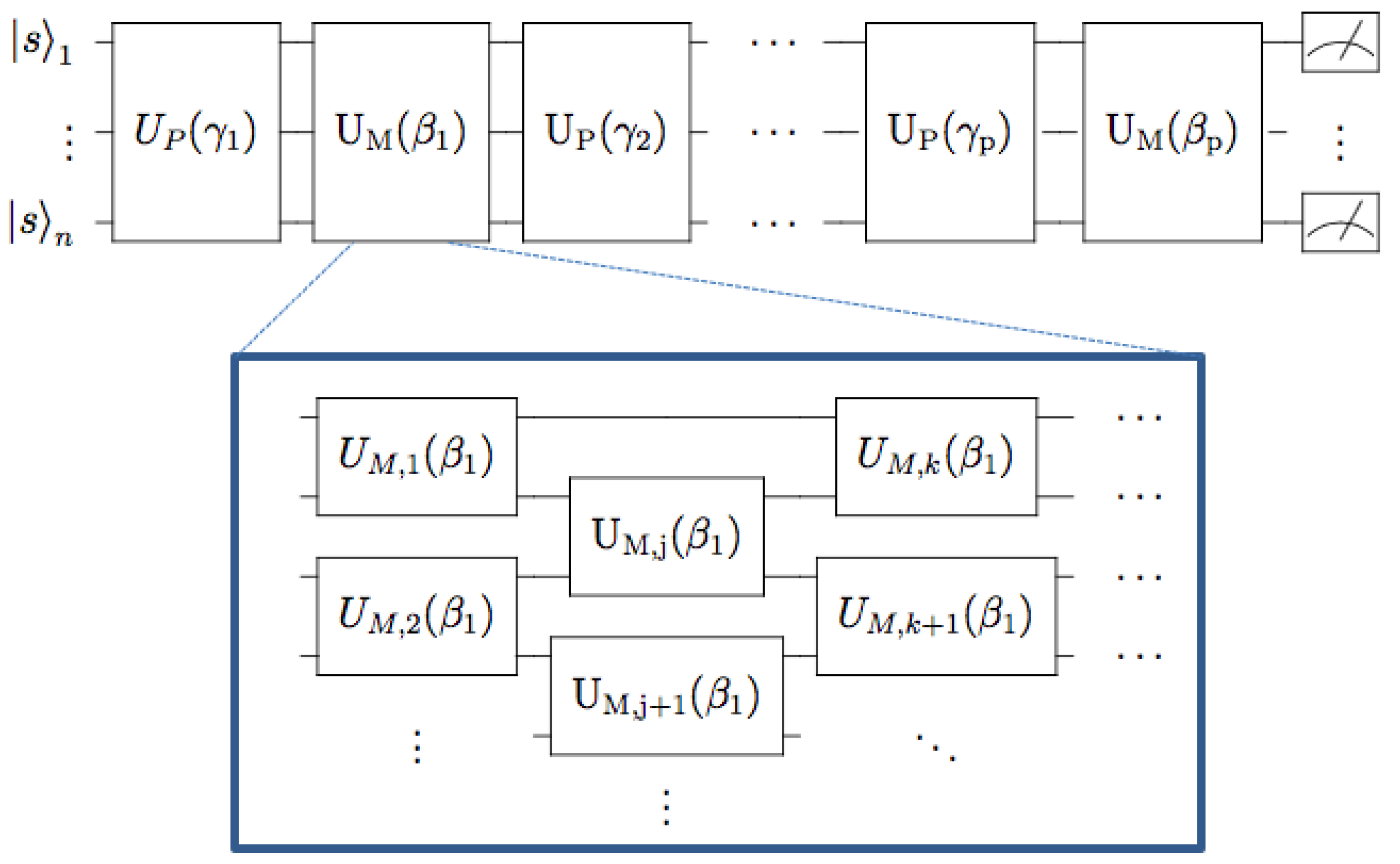
where $\beta$ and $\gamma$ are real parameters. Specifically, a ${\mathrm{QAOA}}_p$ circuit consists of p alternating applications of operators from these two families:

$$Q_p(\mathit{\beta },\gamma )=U_{\mathrm{M}}({\beta }_p)U_{\mathrm{P}}({\gamma }_p)\dots U_{\mathrm{M}}({\beta }_1)U_{\mathrm{P}}({\gamma }_1).$$

(1)

This quantum alternating operator ansatz (QAOA) consists of the states representable as the application of such a circuit to a suitably simple initial state $|s\rangle$:

$$|\mathit{\beta },\gamma \rangle =Q_p(\mathit{\beta },\gamma )|s\rangle .$$

(2)

We show an overall quantum circuit schematic for a QAOA mapping in Figure 1 below. For a given optimization problem, a QAOA mapping of a problem consists of a family of phase-separation operators, a family of mixing operators, and a starting state. The circuits for the original quantum approximate optimization algorithm fit within this paradigm, with unitaries of the form $e^{-i\gamma H_{\mathrm{P}}}$ and $e^{-i\beta H_{\mathrm{M}}}$, with parameters $\gamma$ and $\beta$ indicating the time for which a fixed Hamiltonian is applied.

The domain will usually be expressed as the feasible subset of a larger configuration space, specified by a set of problem constraints. For implementation on expected near-term quantum hardware, each configuration space will need to be encoded into a subspace of a Hilbert space of a multiqubit system, with the domain corresponding to a feasible subspace of the configuration space. For each domain, there are many possible mixing operators. As we will see, using more general one-parameter families of unitaries enables more efficiently implementable mixers that preserve the feasible subspace. Given a domain, an encoding of its configuration space, a phase separator, and a mixer, there are a variety of compilations of the phase separator and mixer to circuits that act on qubits.

For any function f, not just an objective (cost) function, we define $H_f$ to be the quantum Hamiltonian that acts as f on basis states as:

$$H_f|\mathbf{x}\rangle =f(\mathbf{x})|\mathbf{x}\rangle .$$

(3)

In prior work, the domain F was the set of all n-bit strings, $U_{\mathrm{P}}(\gamma )=e^{-i\gamma H_f}$, and $U_{\mathrm{M}}(\beta )=e^{-i\beta H_B}$. Furthermore, with just one exception, the mixing Hamiltonian was $H_B={\sum }_{j=1}^n{X}_j$. We used the notation $X_j$, $Y_j$, $Z_j$ to indicate the Pauli matrices X, Y, and Z acting on the jth qubit. The corresponding parameterized unitaries are denoted by $X_j(\theta )=e^{-i\theta X_j}$ and similarly for $Y_j$ and $Z_j$. The one exception is Section VIII of Reference [1], which discusses a variant for the maximum independent set problem, in which F is the set of bitstrings corresponding to the independent sets of a graph, the phase separator depends on the cost function as above, and the mixing operator is $U_{\mathrm{M}}(\beta )=e^{-i\beta H_B}$, where $H_B$ is such that:

$$\langle \mathbf{x}|H_B|\mathbf{y}\rangle =\left\{\begin{array}{cc}1,\hfill & \mathbf{x},\mathbf{y}\in F\mathrm{and}\mathrm{Ham}(\mathbf{x},\mathbf{y})=1,\hfill \\ 0,\hfill & \mathrm{otherwise},\hfill \end{array}\right.$$

(4)

which connects feasible qubit computational basis states with unit Hamming distance $(\mathrm{Ham})$. Section VIII of Reference [1] does not discuss the implementability of $U_{\mathrm{M}}(\beta )$. A closely related generalization of QAOA for problems with hard constraints based on quantum walks has recently been proposed [31]. However, row-computable feasibility oracles are required to enable mixing between feasible states, which are likely to be more expensive to implement in practice than the approach of this paper.

We extended and formalized the approach of Section VIII of Reference [1] with an eye to implementability, both in the short and long term. We also built on a theory developed for adiabatic quantum optimization (AQO) by Hen and Spedalieri [6] and Hen and Sarandy [7], though the gate-model setting of QAOA leads to different implementation considerations than those for AQO. For example, Hen et al. identified driver Hamiltonians of the form $H_{\mathrm{M}}={\sum }_{j,k}{H}_{j,k}$, where $H_{j,k}=X_j{X}_k+Y_j{Y}_k$, as useful in the AQO setting for a variety of optimization problems with hard and soft constraints; such mixers restrict the mixing to the feasible subspace defined by the hard constraints. Analogously, the unitary $U_{\mathrm{M}}=e^{-i\beta H_{\mathrm{M}}}$ meets our criteria, discussed in Section 3.1, for good mixing for a variety of optimization problems, including those considered in References [6,7]. Since $H_{j,k}$ and $H_{i,l}$ do not commute when $\left|\right\{j,k\}\cap \{i,l\left\}\right|=1$, compiling $U_{\mathrm{M}}$ to two-qubit gates is nontrivial. One could Trotterize, but it may be more efficient and just as effective to use an alternative mixing operator, such as $U_{\mathrm{M}}=e^{-i\beta H_{S_r}}\dots e^{-i\beta H_{S_2}}{e}^{-i\beta H_{S_1}}$, where the pairs of qubits have been partitioned into r subsets ${\left\{S_i\right\}}_i$ containing only disjoint pairs, motivating in part our more general ansatz.

We define as “Hamiltonian-based QAOA” (H-QAOA) the class of QAOA circuits in which both the phase separator family $U_{\mathrm{P}}(\gamma )=e^{-i\gamma H_{\mathrm{P}}}$ and the mixing operator family $U_{\mathrm{M}}(\beta )=e^{-i\beta H_{\mathrm{M}}}$ correspond to time evolution under some Hamiltonians $H_{\mathrm{P}}$ and $H_{\mathrm{M}}$, respectively. (In the example mappings to follow, we consider only phase separators $U_{\mathrm{P}}(\gamma )={\sum }_{\mathbf{x}}{e}^{-i\gamma g(\mathbf{x})}|\mathbf{x}\rangle \langle \mathbf{x}|$ that correspond to classical functions and thus also correspond to time evolution under some (potentially nonlocal) Hamiltonians, though more general types of phase separators may be considered). We further define “local Hamiltonian-based QAOA” (LH-QAOA) as the subclass of H-QAOA in which the Hamiltonian $H_{\mathrm{M}}$ is a sum of (polynomially many) local terms.

Before discussing design criteria, we briefly mention that there are obvious generalizations in which $U_{\mathrm{P}}$ and $U_{\mathrm{M}}$ are taken from families parameterized by more than a single parameter. For example, in Reference [26], a different parameter for every term in the Hamiltonian is considered. In this paper, we only consider the case of one-dimensional families, given that it is a sufficiently rich area of study, with the task of finding good parameters ${\gamma }_1,\dots ,{\gamma }_p$, and ${\beta }_1,\dots ,{\beta }_p$ already challenging enough due to the curse of dimensionality [21]. A larger parameter space may support more effective circuits but increases the difficulty of finding such circuits by opening up the design space and making the parameter setting more difficult.

We remark that the quantum gate-model setting offers several advantages over Hamiltonian-based algorithms such as AQO and quantum annealing. Higher order (k-local) interactions may be compiled down to two-local gates, and compilations using SWAP gates [22,35] enable the implementation of quantum operations between qubits that are non-neighboring in the physical hardware; indeed, locality and connectivity are both well-known bottlenecks for physical quantum annealing devices. In the longer term, once mature quantum hardware has been built, quantum error correction can be applied to robustly implement QAOA.

3.1. Design Criteria

Here, we briefly specify design criteria for the three components of a QAOA mapping of a problem. We expect that as exploration of QAOA proceeds, these design criteria will be strengthened and will depend on the context in which the ansatz is used. For example, when the aim is a polynomial-time quantum circuit, the components should have more stringent bounds on their complexity; without such bounds, the ansatz is not useful as a model for a strict subset of states producible via polynomially-sized quantum circuits. On the other hand, when the computation is expected to grow exponentially, a simple polynomial bound on the depth of these operators might be reasonable. One example might be for exact optimization of the problems considered here; for these problems, the worst case algorithmic complexity is exponential, but it is worth exploring whether QAOA might outperform classical heuristics in expanding the tractable range for some problems.

Initial state. We require that the initial state $|s\rangle$ be trivial to implement, by which we mean that it can be created by a constant-depth (in the size of the problem) quantum circuit from the $|0\dots 0\rangle$ state. Here, we often take as our initial state a single feasible solution, usually implementable by a depth-1 circuit consisting of single-qubit bit-flip operations X. Because in such a case the initial phase operator only applies a global phase, we may want to consider the algorithm as starting with a single-mixing operator $U_{\mathrm{M}}({\beta }_0)$ to the initial state as a first step. In the quantum approximate optimization algorithm, the standard starting state $|+\dots +\rangle$ is obtained by a depth-1 circuit that applies a Hadamard H gate to each of the qubits in the $|0\dots 0\rangle$ state.

This criterion could be relaxed to logarithmic depth if needed. It should not be relaxed too much: Relaxing the criterion to polynomial depth would obviate the usefulness of the ansatz as a model for a strict subset of states producible via polynomially-sized quantum circuits. Algorithms with more complex initial states should be considered hybrid algorithms, with an initialization part and a QAOA part. Such algorithms are of interest in cases when one expects the computation to grow exponentially, such as is the case for exact optimization for many of the problems here, but might still outperform classical heuristics in expanding the tractable range.

Phase-separation unitaries. We require the family of phase-separation operators to be diagonal in the computational basis. In almost all cases, we take $U_{\mathrm{P}}(\gamma )=e^{-i\gamma H_f}$, where f is the objective function.

Mixing unitaries (or “mixers”). We require the family of mixing operators $U_{\mathrm{M}}(\beta )$ to:

• Preserve the feasible subspace: For all values of the parameter $\beta$, the resulting unitary takes feasible states to feasible states, and;
• Provide transitions between all pairs of states corresponding to feasible points. More concretely, for any pair of feasible computational-basis states $\mathbf{x},\mathbf{y}\in F$, there is some parameter value ${\beta }^{\ast }$ and some positive integer r such that the corresponding mixer connects those two states: $\left|〈\mathbf{x}|U_{\mathrm{M}}^r({\beta }^{\ast })|\mathbf{y}〉\right|>0$.

In some cases, we may want to relax some of these criteria. For example, if a QAOA circuit is being used as a subroutine within a hybrid quantum-classical algorithm, or in a broader quantum algorithm, we may use starting states informed by previous runs and thus allow mixing operators that mix less.

This framework can be used in many different contexts. Depending on the context, different measures of success are appropriate. As indicated by the name, the original motivation for Farhi et al.’s work was to develop a quantum approximation algorithm, one for which rigorous bounds on the approximation ratio can be proven [1,16]. The same style of algorithm was then applied to exact optimization [20] and sampling [17], which have different measures of success. In certain cases, rigorous performance guarantees can be provided in these contexts, e.g., for the Grover problem in Reference [19]. Alternatively, it can be applied as a heuristic approach for any of exact optimization, approximate optimization, or sampling. In these cases, the measure of success is not in terms of rigorous analytical bounds, but rather empirical typical time-to-solution or approximation ratio or sample quality within a given time. Our approach facilitates low-resource constructions that support empirical evaluation of QAOA as a heuristic for a variety of combinatorial optimization problems, and is agnostic as to which success criterion is being used for evaluation.

4. QAOA Mappings: Strings

This section describes mappings to QAOA for four problems in which the underlying configuration space is strings with letters taken from some alphabet. We introduce some basic families of mixers and discuss compilations thereof, illustrating their use with MaxColorableSubgraph as an example. We then build on these basic mixers to design families of more complicated mixers, such as controlled versions of these mixers, and illustrate their use in mappings and circuits for the problems MaxIndependentSet, MaxColorableInducedSubgraph, and MinGraphColoring as examples. The mixers we develop in this section, and close variants, are applicable to a wide variety of problems, as we see in Appendix A.

4.1. Example: Max-$\kappa$-ColorableSubgraph

Problem. Given a graph $G=(V,E)$ with n vertices and m edges, and $\kappa$ colors, maximize the size (number of edges) of a properly vertex-$\kappa$-colorable subgraph.

The domain F is the set of colorings $\mathbf{x}$ of G, an assignment of a color to each vertex. (Note that here and throughout, the term “colorings” includes improper colorings.) The domain F can be represented as the set of length n strings over an alphabet of $\kappa$ characters, $\mathbf{x}=x_1{x}_2\dots x_n$, where $x_i\in \left[\kappa \right]$. The objective function $f:{\left[\kappa \right]}^n\to \mathbb{N}$ counts the number of properly colored edges in a coloring:

$$f(\mathbf{x})=\sum _{\{u,v\}\in E}\mathsf{NEQ}(x_u,x_v).$$

(5)

We then built up machinery to define mixing operators for a QAOA approach to this problem. Since some mixing operators are more naturally expressed in one encoding rather than another, we found it useful to describe different mixing operators in different encodings, though we emphasize that doing so is merely for convenience; all mixing operators are encoding-independent, so the descriptions may be translated from one encoding to another. The domain F is naturally expressed as strings of d-dits, a d-valued generalization of bits. For the present problem, $d=\kappa$. In addition to discussing colorings as strings of dits, we used a “one-hot” encoding into $n\kappa$ bits, with $x_{i,c}$ indicating whether or not vertex i is assigned color c.

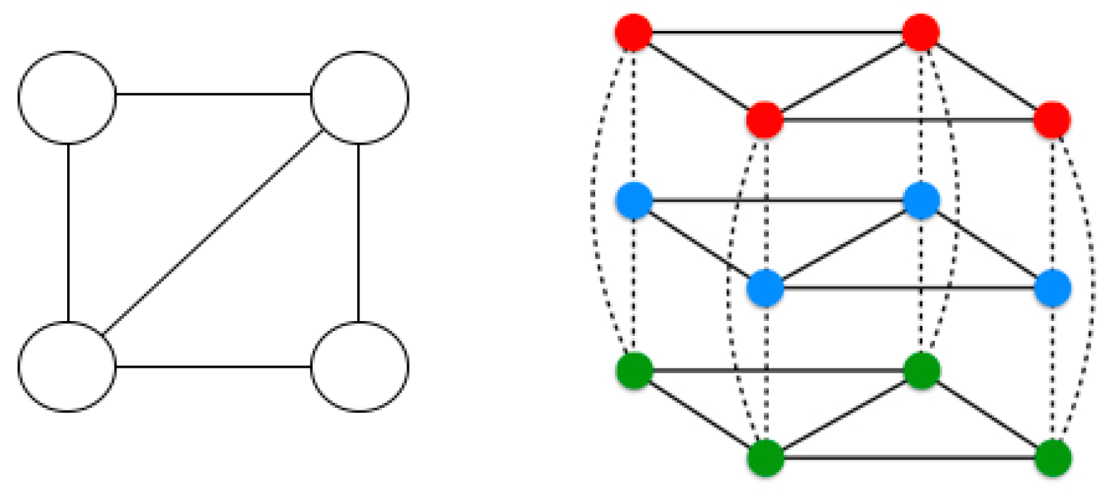
Figure 2 below shows a mapping to qubits in the one-hot encoding for Max-$\kappa$-ColorableSubgraph. We explain this and other possible mappings generally over the remainder of the section.

4.1.1. Single Qudit Mixing Operators

We focused initially on designing partial mixers, component operators that will be used to construct full mixing operators. For this mapping of the maxColorableSubgraph problem, the partial mixers are operators acting on a qudit with dimension $d=\kappa$ that mix between the colors associated to a single vertex v. As we see in subsequent sections, this is a particularly simple case of partial mixers which are often more complicated multiqubit-controlled operators. Once we have defined these single-qudit partial mixing operators, we put them together to create a full mixer for the problem.

We began by considering the following family of single-qudit mixing operators expressed in terms of qudits, and qudit operators, and then considered encodings and compilations to qubit-based architectures, which inspired us to consider other families of single-qubit mixing operators. See Appendix C.2 and References [36,37] for a review of qudit operators, including the generalized Pauli operators $\breve{X}$ and $\breve{Z}$.

r-nearby-values single-qudit mixer. Let $U_{r-\mathrm{NV}}(\beta )=e^{-i\beta H_{r-\mathrm{NV}}}$, where $H_{r-\mathrm{NV}}={\sum }_{i=1}^r\left({\breve{X}}^i+{({\breve{X}}^{†})}^i\right)$, which acts on a single qudit, with $\breve{X}={\sum }_{a=0}^{d-1}|a+1\rangle \langle a|$. We identified two special cases by name: The “single-qudit ring mixer” for $r=1$, $H_{\mathrm{ring}}=H_{1-\mathrm{NV}}$ and the “fully-connected” mixer for $r=d-1$, $H_{\mathrm{FC}}=H_{(d-1)-\mathrm{NV}}$. Whenever we introduced a Hamiltonian, we also implicitly introduced its corresponding family of unitaries, as with $H_{r-\mathrm{NV}}$ and $U_{r-\mathrm{NV}}(\beta )$.

The single-qudit ring mixer is a cornerstone of many of the mixing constructions that we discuss. We concentrated on qubit encodings thereof, given the various projections of hardware with at least 40 qubits that will be available in the next year or two [11,12], though it could alternatively be implemented directly using a qudit-based architecture. We explored two natural encodings of a qudit into qubits: (1) The one-hot encoding using d qubits, in which each qudit basis state $|a\rangle$, $a=0,1,\dots ,d-1$, is encoded as ${|0\rangle }^{\otimes a}\otimes |1\rangle \otimes {|0\rangle }^{\otimes d-1-a}$; and (2) the binary encoding using $\lceil {log}_{2}d\rceil$ qubits, in which each qudit state $|a\rangle$ is encoded as the qubit computational basis state labeled by the binary representation of the integer a. The one-hot encoding uses more qubits but supports a simpler compilation of the single-qudit ring mixer for general d, both in the sense of it being much easier to write down a compilation, and in the sense that it uses many fewer two-qubit gates; in the one-hot encoding, 2-local mixing interactions suffice, whereas binary encoding requires $\lceil {log}_{2}d\rceil$-local Hamiltonian terms, with the corresponding unitary requiring further compilation to two-qubit gates.

In the one-hot encoding, the single-qudit ring mixer is encoded as a qubit unitary $U_{\mathrm{ring}}^{(\mathrm{enc})}$ corresponding to the qubit Hamiltonian:

$$H_{\mathrm{ring}}^{(\mathrm{enc})}=\sum _{a=0}^{d-1}\left(X_a{X}_{a+1}+Y_a{Y}_{a+1}\right),$$

(6)

which acts on the qubit Hilbert space in a way that preserves the Hamming weight of computational basis states and acts as $U_{\mathrm{ring}}$ on the encoded subspace spanned by unit Hamming weight computational basis states.

Although $H_{\mathrm{ring}}^{(\mathrm{enc})}$ is 2-local, its terms do not mutually commute. There are several implementation options. First, hardware that natively implements the multiqubit gate $U_{\mathrm{ring}}^{(\mathrm{enc})}$ directly may be plausible (much as quantum annealers already support the simultaneous application of a Hamiltonian to a large set of qubits), but most proposals for universal quantum processors are based on two-qubit gates, so a compilation to such gates is desirable both for applicability to hardware likely to be available in the near term and for error-correction and fault tolerance in the longer term. Second, we could use constructions used in quantum many-body physics to compile $U_{\mathrm{ring}}^{(\mathrm{enc})}$ into a circuit of 2-local gates [38]. Third, the multiqubit gate $U_{\mathrm{ring}}^{(\mathrm{enc})}$ could be implemented approximately via Trotterization or other Hamiltonian simulation algorithms. A different approach, and the alternative we explore most extensively here, is to implement a different unitary rather than $U_{r-\mathrm{NV}}$, one related to $U_{r-\mathrm{NV}}$, and sharing its desirable mixing properties, as encapsulated in the design criteria of Section 3.1, which is easier to implement. The form of the circuit obtained by Trotterization is suggestive. We considered sequentially applying unitaries corresponding to subsets of terms in the Hamiltonian, each subset chosen in such a way that the corresponding unitary is readily implementable. This reasoning mirrors the relation of H-QAOA circuits to Trotterized AQO. We give a few examples of mixers obtained in this way.

Parity single-qudit ring mixer. Still in the one-hot encoding, we partitioned the d terms $e^{-i\beta \left(X_a{X}_{a+1}+Y_a{Y}_{a+1}\right)}$ by the parity of their indices. Let:

$$U_{\mathrm{parity}}(\beta )=U_{\mathrm{last}}(\beta )U_{\mathrm{even}}(\beta )U_{\mathrm{odd}}(\beta ),$$

(7)

where:

$$\begin{array}{cccc}\hfill U_{\mathrm{odd}}(\beta )& =\prod _{a\mathrm{odd},a\ne n}{e}^{-i\beta \left(X_a{X}_{a+1}+Y_a{Y}_{a+1}\right)},\hfill & \hfill U_{\mathrm{even}}(\beta )& =\prod _{a\mathrm{even}}{e}^{-i\beta \left(X_a{X}_{a+1}+Y_a{Y}_{a+1}\right)},\hfill \end{array}$$

(8)

$$\begin{array}{cc}\hfill U_{\mathrm{last}}(\beta )& =\left\{\begin{array}{cc}{e}^{-i\beta \left(X_d{X}_1+Y_d{Y}_1\right)},\hfill & d\mathrm{odd},\hfill \\ I,\hfill & d\mathrm{even}.\hfill \end{array}\right.\hfill \end{array}$$

(9)

Such “XY” gates are natively implemented on certain superconducting processors [39].

It is easy to see that the parity single-qudit ring mixer preserves the Hamming weight and hence meets the first criterion of keeping the evolution within the feasible single-qudit subspace. To see that it also meets the second, providing transitions between all feasible computational basis states, it is useful to consider the quantum swap gate, which behaves in exactly the same way as the XY gate on the subspace spanned by $\left\{|0_i{1}_j\rangle ,|1_i{0}_j\rangle \right\}$. The swap gate ${\mathrm{SWAP}}_{i,j}=\frac{1}{2}(I+X_i{X}_j+Y_i{Y}_j+Z_i{Z}_j)$ is both unitary and Hermitian, and thus:

$$e^{i\theta {\mathrm{SWAP}}_{i,j}}=cos(\theta )I+isin(\theta ){\mathrm{SWAP}}_{i,j}.$$

(10)

For $0<\beta <\pi /2$, each term in the parity single-qudit ring mixer is a superposition of a swap gate and the identity. A single application of $U_{\mathrm{parity}}(\beta )$ will have nonzero transition amplitudes only between pairs of colors with indices no more than two apart. Nevertheless, this mixer meets the second criteria because all possible orderings of d swap gates appear in $\lceil \frac{d}{2}\rceil$ repeats of the parity operator for any $0<\beta <\pi /2$, thus providing nonzero amplitude transitions between all feasible computational basis states for a single-vertex graph.

When d is an integer power of two, there is also a straightforward, though more resource-intensive, compilation of the parity single-qudit ring mixer using the binary encoding. Applying a Pauli X gate to the least-significant qubit acts as $H_{\mathrm{even}}$ on the encoded subspace. Incrementing the register by one, applying the Pauli gate to the least-significant qubit, and finally decrementing the register by one overall acts as $H_{\mathrm{odd}}$. Therefore, we can implement $U_{\mathrm{parity}}$ by incrementing the register by one, applying an $X(\beta )=e^{-i\beta X}$ to the least-significant qubit, decrementing the register by one, and then again applying an $X(\beta )$ gate to the least-significant qubit. For an l-bit register, each incrementing and decrementing operation can be written as a series of l multiply-controlled X gates, with the numbers of control ranging from 0 to $l-1$.

Repeated parity single-qudit ring mixers. As we mentioned above, a single application of $U_{\mathrm{parity}}(\beta )$ will have nonzero transition amplitudes only between pairs of colors with indices no more than two apart, which suggests that it may be useful to repeat the parity mixer within one mixing step.

Partition single-qudit ring mixers. We now generalize the above construction for the parity single-qudit ring mixer to more general partition mixers. For a given ordered partition $\mathcal{P}=(P_1,\dots ,P_p)$ of the terms of $H_{r-\mathrm{NV}}$ such that all pairs of terms within a $P_i$ act on disjoint states of the qudit, let:

$$U_{\mathcal{P}-r-\mathrm{NV}}(\beta )=U_{P_p-\mathrm{XY}}(\beta )\dots U_{P_1-\mathrm{XY}}(\beta ),$$

(11)

where:

$$U_{P-\mathrm{XY}}(\beta )=\prod _{\{a,b\}\in P}{e}^{-i\beta \left(|a\rangle \langle b|+|b\rangle \langle a|\right)}.$$

(12)

By construction, in the one-hot encoding, the terms of $U_{P-\mathrm{XY}}$ commute (because they act on disjoint pairs of qubits), and so the ordering does not matter; all can be implemented in parallel. We call $U_{\mathcal{P}-r-\mathrm{NV}}$ the “partition $\mathcal{P}$” r-nearby-values single-qudit ring mixer, and $U_{r-\mathrm{NV}}$ the “simultaneous” r-nearby-values single-qudit ring mixer to distinguish the latter from the former. The latter is member of H-QAOA, while the former is not.

Even more generally, for a set of single-qudit ring mixers $\left\{H_{\alpha }\right\}$ indexed by some $\alpha$ and an ordered partition $\mathcal{P}=(P_1,\dots ,P_p)$ thereof, in which the single-qudit mixers within each part mutually commute, we defined a simultaneous version, $e^{-i\beta {\sum }_{\alpha }{H}_{\alpha }}$ and a $\mathcal{P}$-partitioned version, ${\prod }_{i=1}^P\left[{\prod }_{\alpha \in P_i}{e}^{-i\beta H_{\alpha }}\right]$, where the order of the product over the elements of each part does not matter because they commute, and the order of the product over the parts of the partition is given by their ordering within the ordered partition $\mathcal{P}$.

Binary single-qudit mixer for $d=2^l$. We now return briefly to the binary encoding, and describe a different single-qudit mixer. An alternative to the r-nearby values single-qudit mixer, which is easily implementable using the binary encoding when $d=2^l$ is a power of two, is the “simple binary” single-qudit mixer:

$$H_{\mathrm{binary}}^{(\mathrm{enc})}=\sum _{i=1}^l{X}_i,$$

(13)

where $X_i$ acts on the ith qubit in the binary encoding of the qudit. Since the ordering of the colors was arbitrary to begin with, it does not much matter whether the Hamiltonian mixes nearby values in the ordering or mixes the colors in a different way, in this case to colors with indices whose binary representations have Hamming distance 1.

When d is not a power of 2, a straightforward generalization of the binary single-qudit mixer experiences difficulty in meeting the first of the design criteria, since swapping one of the bit values in the binary representation may take the evolution out of the feasible subspace. While requiring d to be a power of 2 restricts its general applicability, the binary single-qudit mixer could be useful in some interesting cases, such as 4-coloring. For 2-coloring (a problem equivalent to MaxCut), the full binary single-qudit mixer is simply the standard mixer X. We use this encoding in Section 5.2 to handle slack variables in a single-machine scheduling problem, a case in which there is flexibility in the upper range of the integer to be encoded, allowing us to round up to the nearest power of two when needed.

4.1.2. Full QAOA Mapping

Having introduced several partial mixers for single qudits, we now show a complete QAOA circuit for MaxColorableSubgraph with n vertices, m edges, and $\kappa$ colors, compiled to 2-local gates on qubits. Using the one-hot encoding, we require $n\kappa$ qubits.

Mixing operator. We used as the full mixer a parity ring mixer made up of parity single-qudit ring mixers, one for each of the qudits corresponding to each vertex:

$$U_{\mathrm{M}}=\prod _{v=1}^n{U}_{v,\mathrm{parity}}^{(\mathrm{enc})}.$$

(14)

The single qubit mixers act on different qubits and can be applied in parallel. The overall parity mixing operator required a depth-2 or depth-3 circuit (for even and odd $\kappa$, respectively) of $n\kappa$ gates. Other single-qudit mixers we defined above, including r repeats of the parity ring mixer, other partitioned mixers, or the binary mixer, could be used in place of the parity single-qudit mixer in this construction. All of these unitary mixers by construction meet our first criterion for a mixer: Keeping the evolution in the feasible subspace. Further, each of these mixers, after at most $\lceil \frac{\kappa }{2}\rceil$ repeats, provides nonzero amplitude transitions between all colors at a given vertex, with the product providing transitions between any two feasible states.

Phase-separation operator. The objective function can be written in classical one-hot encoding as:

$$m-\sum _{\{u,v\}\in E}\sum _{a=1}^k{x}_{u,a}{x}_{v,a},$$

(15)

where $x_{v,a}=1$, indicating that vertex v has been assigned color a. To obtain a phase-separation Hamiltonian, we substituted $(I-Z)/2$ for each binary variable to obtain:

$$H_{\mathrm{P}}^{\prime }=\frac{4-\kappa }{4}mI+\frac{1}{4}\sum _{\{u,v\}\in E}\sum _{a=1}^{\kappa }\left(Z_{u,a}+Z_{v,a}-Z_{u,a}{Z}_{v,a}\right).$$

(16)

The constant term affects only a physically-irrelevant global phase, and since we are only concerned about the feasible subspace, we can disregard each sum ${\sum }_{a=1}^{\kappa }{Z}_{u,a}$ of all $\kappa$ single Z operators corresponding to a single qudit, since they multiply each of the d Hamming weight 1 elements corresponding to the d single qudit values by the same constant, resulting in a global phase. Removing those terms and rescaling, the phase separator now has the simpler form:

$$H_{\mathrm{P}}^{(\mathrm{enc})}=\sum _{\{u,v\}\in E}\sum _{a=1}^{\kappa }{Z}_{u,a}{Z}_{v,a},$$

(17)

where $Z_{v,a}$ acts on the ath qubit in the one-hot encoding of the vth qudit, corresponding to coloring vertex v with color a. The phase separator requires a circuit containing $m\kappa$ two-qubit gates with depth at most $D_G+1$, where $D_G$ is the maximum degree over all vertices in the instance graph G.

Translated back to acting on qudits, Equation (17) acts as $H_{\mathrm{P}}=H_g$ (as defined in Equation (3)), where $g(\mathbf{x})=\kappa m-4f(\mathbf{x})$. We refer to this function g as the “phase function”, which will typically be an affine transformation of the objective function, which corresponds simply to a physically irrelevant global phase and a rescaling of the parameter. Defining $H_{\mathrm{P}}$ using such a phase function allows us to write a simpler encoded version $H_{\mathrm{P}}^{(\mathrm{enc})}$ that corresponds exactly to $H_{\mathrm{P}}$, without qualification, on the encoded subspace.

Initial state. Any encoded coloring can be generated by a depth-1 circuit of at most n single-qubit X gates. A reasonable initial state is one in which all vertices are assigned the same color. Alternatively, we could start with any other feasible state, or the initial state could be obtained by applying one or more rounds of the mixer to a single feasible state, so that the algorithm begins with a superposition of feasible states.

The circuit depth and gate count for the full algorithm will increase when compiling to realistic near-term hardware with architectures that have nearest neighbor topological constraints limiting between which pairs of physical qubits two-qubit gates can be applied. See Reference [22] for one approach for compiling to realistic hardware with such constraints.

Further investigation is needed to understand which mixers and initial states, for a given resource budget, result in more or less effective algorithms, and whether some have an advantage with respect to finding good parameters ${\gamma }_1,\dots ,{\gamma }_p$, and ${\beta }_1,\dots ,{\beta }_p$ or being robust to error.

4.2. Example: MaxIndependentSet

Problem. Given a graph $G=(V,E)$, with $\left|V\right|=n$ and $\left|E\right|=m$, find the largest subset $V^{\prime }\subset V$ of mutually non-adjacent vertices.

This problem was discussed in Section VII of Reference [1] as a “variant” of the quantum approximate optimization algorithm introduced in that paper. To handle this problem, Farhi et al. suggested restricting the evolution to what we are calling the feasible subspace of the overall Hilbert space, the subspace spanned by computational basis elements corresponding to independent sets, through modification of what we are calling the mixing operator. We made the construction of the H-QAOA mixer Farhi et al. defined more explicit, and introduced partitioned mixers that have implementation advantages over the H-QAOA, or simultaneous, mixer defined in Farhi et al.

The configuration space is the set of n-bit strings, representing subsets $V^{\prime }\subset V$ of vertices, where $i\in V^{\prime }$ if and only if $x_i=1$. The domain F is represented by the subset of all n-bit strings corresponding to independent sets of G. In contrast to the domain for MaxColorableSubgraph, this domain is dependent on the problem instance, not just on the size of the problem. Because the configuration is already bit-based, some aspects of mapping this problem to QAOA are simpler, but the partitioned mixing operators are more complicated in that they require controlled operation.

To support the discussion of controlled operators, we used the notation ${\Lambda }_{\mathbf{y}}(Q)$ to indicate a unitary target operator Q applied to a set of target qubits controlled by the state $\mathbf{y}$ of a set of control qubits:

$${\Lambda }_{\mathbf{y}}(Q)=\sum _{{\mathbf{y}}^{\prime }\ne \mathbf{y}}|{\mathbf{y}}^{\prime }\rangle \langle {\mathbf{y}}^{\prime }|\otimes I+|\mathbf{y}\rangle \langle \mathbf{y}|\otimes Q.$$

(18)

More generally, we used ${\Lambda }_{\chi }(Q)$ when the operation was controlled on a predicate $\chi$:

$${\Lambda }_{\chi }(Q)=\sum _{\mathbf{y}:\neg \chi (\mathbf{y})}|\mathbf{y}\rangle \langle \mathbf{y}|\otimes I+\sum _{\mathbf{y}:\chi (\mathbf{y})}|\mathbf{y}\rangle \langle \mathbf{y}|\otimes Q.$$

(19)

Whether the subscript of $\Lambda$ is a string or predicate will be clear from context. For a Hamiltonian $H_Q$ such that $Q=e^{-i{H}_Q}$, we can write the controlled unitary Equation (19) as:

$${\Lambda }_{\chi }(Q)=e^{-i{H}_{\chi }\otimes H_Q}.$$

(20)

We refer to $H_{\chi }\otimes H_Q$ as the controlled Hamiltonian, $\chi$-controlled-$H_Q$. Note that the Hamiltonian $H_{\chi }$ that acts as the predicate $\chi$ on computational basis states, in the sense of Equation (3), is precisely the projector $H_{\chi }={\sum }_{\mathbf{x}:\chi (\mathbf{x})=1}|\mathbf{x}\rangle \langle \mathbf{x}|$ that projects onto the subspace on which the predicate is 1. We used this relation to connect corresponding controlled Hamiltonians and controlled unitaries. In particular, when we want to apply a phase only on the part of the Hilbert space picked out by a predicate $\chi$, we can write:

$${\Lambda }_{\chi }\left(e^{-i\theta }\right)=e^{-i\theta H_{\chi }},$$

(21)

where we have adapted the control notation of Equation (20) to mean applying the operator $Q=e^{-i\theta }$ to zero target qubits. We often compile controlled unitaries (both phase separators and mixers) by using ancilla qubits to intermediate the control, e.g., for a single ancilla qubit (initialized at $|0\rangle$ and returned thereto):

$${\left({\Lambda }_{\chi }\left(Q\right)\right)}^{(\mathrm{comp})}={\Lambda }_{\chi }\left(X_{\mathrm{anc}}\right){\Lambda }_{x_{\mathrm{anc}}}\left(Q\right){\Lambda }_{\chi }\left(X_{\mathrm{anc}}\right).$$

(22)

We explore in detail the construction of such controlled Hamiltonians and unitaries in Reference [5].

4.2.1. Partial Mixing Operator at Each Vertex

Given an independent set $V^{\prime }$, we can add a vertex $w\notin V^{\prime }$ to $V^{\prime }$ while maintaining feasibility only if none of its neighboring vertices $\mathrm{nbhd}(w)$ are already in $V^{\prime }$. On the other hand, we can always remove any vertex $w\in V^{\prime }$ without affecting feasibility. Hence, a bit-flip operation at a vertex, controlled by its neighbors (adjacent vertices), suffices both to remove and add vertices while maintaining the independence property. These classical moves inspire the controlled-bit-flip partial mixing operators.

In general, for a string $\mathbf{y}$ and a set of indices V, let ${\mathbf{y}}_V={\left(y_{v_i}\right)}_{i=1}^{\left|V\right|}$ be the substring of $\mathbf{y}$ in lexicographical order of the indices. In particular, let ${\mathbf{x}}_{\mathrm{nbhd}(v)}={\left(x_w\right)}_{w\in \mathrm{nbhd}(v)}$. (The ordering of the characters within the substring is arbitrary, because we only use this as the argument to predicates that are symmetric under permutation of the arguments.) For each vertex, we defined the partial mixer as a multiply-controlled X operator:

$$\begin{array}{c}\hfill \begin{array}{ll}{H}_{\mathrm{CX},v}& =X_v{H}_{\mathsf{NOR}(x_{\mathrm{nbhd}(v)})}\\ & =2^{-D_v}{X}_v{\displaystyle \prod _{w\in \mathrm{nbhd}(v)}}(I+Z_w),\end{array}\end{array}$$

(23)

with corresponding partial mixing unitary, a multiply-controlled-$X(\beta )$ single-qubit rotation:

$$\begin{array}{c}\hfill \begin{array}{ll}{U}_{\mathrm{CX},v}(\beta )& =e^{-i\beta H_{\mathrm{CX},v}}\\ & ={\Lambda }_{\mathsf{NOR}(x_{\mathrm{nbhd}(v)})}\left(e^{-i\beta X_v}\right)\hfill \\ & ={\Lambda }_{\mathsf{NOR}(x_{\mathrm{nbhd}(v)})}\left(X_v(\beta )\right),\hfill \end{array}\end{array}$$

(24)

where $X_v(\beta )$ is the single-qubit operator $X_v(\beta )=e^{-i\beta X_v}$. Since $X_v$ is both Hermitian and unitary, $e^{-i\beta X_v}$ is a linear combination of the identity and $X_v$ for $0<\beta <\pi /2$.

4.2.2. Full QAOA Mapping

Mixing operators. Let $H_{\mathrm{CX}}={\sum }_{i=1}^n{H}_{\mathrm{CX},v_i}$. We defined two distinct types of mixers:

• The simultaneous controlled-X mixer, $U_{\mathrm{sim}-\mathrm{CX}}(\beta )=e^{-i\beta H_{\mathrm{CX}}}$, and;
• A class of partitioned controlled-$X(\beta )$ mixers, $U_{\mathcal{P}-\mathrm{CX}}(\beta )={\prod }_{i=1}^{\left|\mathcal{P}\right|}{\prod }_{v\in P_i}{U}_{\mathrm{CX},v}$,

where $\mathcal{P}$ is an ordered partition of the partial mixers, in which each part contains mutually commuting partial mixers. Since the partial mixers often do not commute, different ordered partitions often result in different mixers. By design, both the simultaneous and partitioned mixers restrict evolution to the feasible subspace. With respect to the second design criterion, there is nonzero transition amplitude from the ${|0\rangle }^{\otimes n}$ state corresponding to the empty set to all other independent sets; for $0<\beta <\pi /2$, we got terms corresponding to products of the individual control-bit-flip operators for all subsets of vertices, including those corresponding to independent sets. (For those subsets S not corresponding to independent sets, the product will result in a independent set $V^{\prime }\in S$ that does not include vertices in S which have neighbors whose controlled-bit-flip preceded them in the partition order; thus, different ordered partition affects the amount of nonzero amplitude in the states corresponding to independent sets.) Two applications of any such partitioned mixer result in nonzero amplitude between any two feasible states. An interesting question is how different ordered partitions affect the ease with which good parameters can be found and the quality of the solutions obtained.

Partitioned mixers are generally easier to compile than the simultaneous mixer, since the partitioned mixer is a product of multiqubit-controlled-not operators (generalized Toffoli gates) on at most $D_G+1$ qubits. Altogether, this construction uses n partial mixers, which can then be compiled into single- and two-qubit gates. For many graphs, partitions in which each set contains multiple commuting partial mixers exist, reducing the depth.

Phase-separation operator. The objective function is the size of the independent set, or $f(\mathbf{x})={\sum }_{i=1}^n{x}_i$, which we could translate into a phase-separating Hamiltonian via substitution of $(I-Z)/2$ for each binary variable. Instead, we used affine transformation of the objective function $g(\mathbf{x})=n-2f(\mathbf{x})$, which, when translated, yields a phase separation operator of a simpler form:

$$U_{\mathrm{P}}(\gamma )=e^{-i\gamma H_g}=\prod _{i=1}^n{e}^{-i\gamma Z_i},$$

(25)

which is simply a depth-1 circuit of n single-qubit Z-rotations.

Initial state. A reasonable initial state is the trivial state $|s\rangle ={|0\rangle }^{\otimes n}$ corresponding to the empty set.

4.3. Example: MaxColorableInducedSubgraph

Problem. Given $\kappa$ colors, and a graph $G=(V,E)$ with n vertices and m edges, find the largest induced subgraph that can be properly $\kappa$-colored.

The induced subgraph of a graph $G=(V,E)$ for a subset of vertices $W\subset V$ is the graph $H=(W,E_W)$, where $E_W=\{\{v,w\}\in E:v,w\in W\}$. The configuration space is the set ${[\kappa +1]}^n$ of $(\kappa +1)$-dit strings of length n, corresponding to partial $\kappa$-colorings of the graph: $x_v=0$ indicates that vertex v is uncolored and $x_v=c>0$ indicates that the vertex has color c. The induced subgraph is defined by the colored vertices. The domain is the set of proper partial colorings, those in which two colored vertices that are adjacent in G have different colors. The objective function $f:{[\kappa +1]}^n\to \mathbb{N}$ is the number of vertices that are colored:

$$f(\mathbf{x})=\sum _v\mathsf{NEQ}(x_v,0).$$

(26)

4.3.1. Controlled Null-Swap Mixer at a Vertex

The controlled null-swap partial mixer we defined has elements of the mixers we saw for the previous two problems, combining the control by vertex neighbors from MaxIndependentSet and the color swap from MaxColorableSubgraph. Here, however, we made substantial use of the uncolored state, and at each vertex only considered swapping a color with uncolored status. An uncolored vertex can be assigned color c, maintaining feasibility, as long as none of its neighbors are colored c, whereas uncoloring a vertex always preserves feasibility. This suggests a mixer may be obtained by swaps between each color and the uncolored state, controlled for each vertex by the colors of its neighboring vertices to ensure feasibility. This reasoning in terms of classical moves inspires, for problems containing $\mathsf{NEQ}$ constraints, the controlled null-swap partial mixing Hamiltonian:

$$\begin{array}{ll}{H}_{\mathrm{NS},v,a}& =\left(|a\rangle {\langle 0|}_v+|0\rangle {\langle a|}_v\right)H_{\mathsf{NONE}({\mathbf{x}}_{\mathrm{nbhd}(v)},a)}\\ & =\left(|a\rangle {\langle 0|}_v+|0\rangle {\langle a|}_v\right){\displaystyle \prod _{w\in \mathrm{nbhd}(v)}}\left(I_w-|a\rangle {\langle a|}_w\right),\end{array}$$

(27)

with corresponding controlled null-swap-rotation mixing unitary:

$$U_{\mathrm{NS},v,a}(\beta )={\Lambda }_{\mathsf{NONE}({\mathbf{x}}_{\mathrm{nbhd}(v)},a)}\left(e^{-i\beta \left(|a\rangle {\langle 0|}_v+|0\rangle {\langle a|}_v\right)}+\sum _{b\notin \{0,a\}}|b\rangle {\langle b|}_v\right),$$

(28)

where:

$$\mathsf{NONE}(\mathbf{y},A)=\underset{\begin{array}{c}y\in \mathbf{y}\\ a\in A\end{array}}{\bigwedge }\mathsf{NEQ}(y,a)=\underset{a\in A}{\bigwedge }\underset{i=1}{\overset{\left|\mathbf{y}\right|}{\bigwedge }}\mathsf{NEQ}(y,a)=\underset{a\in A}{\bigwedge }\underset{i\in \left[\left|\mathbf{y}\right|\right]}{\bigwedge }\mathsf{NEQ}(y,a)$$

(29)

is shorthand for none of the variables in $\mathbf{y}$ having value any of the values in A; when $A=\left\{a\right\}$ is a singleton set, we write simply $\mathsf{NONE}(\mathbf{y},a)=\mathsf{NONE}(\mathbf{y},\{a\})$.

4.3.2. Full QAOA Mapping

Mixing operators. Define:

$$H_{\mathrm{NS}}=\sum _{i=1}^n\sum _{a=1}^{\kappa }{H}_{\mathrm{NS},i,a}.$$

(30)

We defined two distinct types of mixers:

• The simultaneous controlled null-swap mixer, $U_{\mathrm{sim}-\mathrm{NS}}(\beta )=e^{-i\beta H_{\mathrm{NS}}}$, and;
• A family of partitioned controlled null-swap mixers, $U_{\mathcal{P}-\mathrm{NS}}(\beta )={\prod }_{a=1}^{\kappa }{\prod }_{i=1}^{\left|\mathcal{P}\right|}{\prod }_{v\in P_i}{U}_{\mathrm{NS},v,a}$.

Again, we have a variety of partitioned mixers, each specified by an ordered partition $\mathcal{P}$ of the vertices such that for each color the terms corresponding to the vertices in the partition commute. We segregated the colors into separate stages, but other orderings are possible.

We used the one-hot encoding of Section 4.1, but with additional variables $x_{v,0}$ for the uncolored states: The binary variables for each vertex v are $x_{v,0},x_{v,1},\dots ,x_{v,k}$. This encoding uses $n(\kappa +1)$ computational qubits. In this encoding, a single partial mixer has the form:

$$\begin{array}{cc}\hfill U_{\mathrm{NS},v,a}^{(\mathrm{comp})}(\beta )& ={\Lambda }_{\mathsf{NOR}({\overline{\mathbf{x}}}_{\mathrm{nbhd}(v),a})}\left(e^{-i\beta \left(X_{v,0}{X}_{v,a}+Y_{v,a}{Y}_{v,0}\right)}\right),\hfill \end{array}$$

(31)

where ${\overline{\mathbf{x}}}_{\mathrm{nbhd}(v),a}={\left(x_{w,a}\right)}_{w\in \mathrm{nbhd}(v)}$. Reasoning similar to that we used for the mixers discussed for the MaxIndependentSet and MaxColorableSubgraph problems shows that this mixer has nonzero transition amplitude between any feasible computational-basis state and the trivial state corresponding to the empty set as the induced subgraph. Two applications of this mixer give nonzero transition amplitudes between any two feasible computational-basis states.

To ease compilation, each partial mixer can be implemented as:

$$U_{\mathrm{NS},v,a}^{(\mathrm{comp})}(\beta )={\Lambda }_{\mathsf{NOR}({\overline{\mathbf{x}}}_{\mathrm{nbhd}(v),a})}\left(X_{\mathrm{anc}}\right){\Lambda }_{x_{\mathrm{anc}}}\left(e^{-i\beta \left(X_{v,0}{X}_{v,a}+Y_{v,a}{Y}_{v,0}\right)}\right){\Lambda }_{\mathsf{NOR}({\overline{\mathbf{x}}}_{\mathrm{nbhd}(v),a})}\left(X_{\mathrm{anc}}\right),$$

(32)

where the control is intermediated by an ancilla qubit, which is initialized and returns to the zero state. Altogether, this construction uses $\kappa n$ partial mixers, which can then be compiled into single- and two-qubit gates. For many graphs, partitions in which each set contains multiple commuting partial mixers exist, reducing the depth.

Phase-separation operator. We can translate the objective function to a Hamiltonian as usual, or translate a linear modification of the objective function to obtain a simpler form. The phase separator function $g(\mathbf{x})=n-2f(\mathbf{x})$ yields the simple phase separator Hamiltonian:

$$H_{\mathrm{P}}^{(\mathrm{comp})}=\sum _v{Z}_{v,0},$$

(33)

for which the corresponding unitary operator can be implemented using a depth-1 circuit of n single-qubit Z-rotations.

Initial state. A reasonable initial state is $|s\rangle ={\left(|1\rangle \otimes {|0\rangle }^{\otimes \kappa }\right)}^{\otimes n}$, corresponding to all vertices uncolored.

4.4. Example: MinGraphColoring

Problem. Given a graph $G=(V,E)$, find the minimal number of colors $k^{\ast }$ required to properly color it.

A graph that can be $\kappa$-colored but not $(\kappa -1)$-colored is said to have chromatic number $\kappa$. We took as our configuration space the set of $\kappa$-dit strings of length n, where $\kappa =D_G+2$. The domain F is the set of proper colorings, many of which will use fewer than $\kappa$ colors. With $D_G+2$ colors, as we explain next, it is possible to get from any proper coloring to any other by local moves while staying in the feasible subspace, a property we made use of in designing mixing operators. We comment that it may be advantageous to take use a larger number of colors since that may promote mixing, but the tradeoffs there would need to be determined in a future investigation.

It is easy to see that any graph can be colored with $D_G+1$ colors. To see that $\kappa =D_G+2$ suffices to get between any two $D_G+1$ colorings, first recognize that given a $D_G+2$ coloring, one can always obtain a $D_G+1$ coloring by simply choosing a color and recoloring each vertex currently colored in that color with one of the other colors, since at least one of those colors will not be used by its neighbors. This move is local, in that it depends only on the neighborhood of the vertex. Now, given two $D_G+1$ colorings C and $C^{\prime }$, we iterated through colors c to tranform between the two colorings via local moves while staying in the feasible space. Let $S^{\prime }\subset V$ be the set of vertices colored c in $C^{\prime }$, and let $S\subset S^{\prime }$ be the set of vertices in $S^{\prime }$ that are not colored c in C. Consider all neighbors of vertices in S. For any neighbor colored c, color it with the unused color. We are now free to color all vertices in S with color c. Iterating through the $\kappa$ colors provides a means of getting from one $D_G+1$ coloring to another by local moves that remain in the feasible space.

4.4.1. Partial Mixer at a Vertex

We used a controlled version of the mixer in Section 4.1 that allows a vertex to change colors only when doing so would not result in an improper coloring; we may swap colors a and b at vertex v only if none of its neighbors are colored a or b. The partial mixer we defined has a similar form to the controlled null-swap partial mixer defined in Equations (27) and (28) but supports color changes between any two colors at a vertex, rather than only between colored and uncolored. Define the controlled-swap partial mixing Hamiltonian:

$$\begin{array}{ll}{H}_{\mathrm{CS},v,\{a,b\}}& =\left(|a\rangle {\langle b|}_v+|b\rangle {\langle a|}_v\right)H_{\mathsf{NONE}({\mathbf{x}}_{\mathrm{nbhd}(v)},\{a,b\})}\\ & =\left(|a\rangle {\langle b|}_v+|b\rangle {\langle a|}_v\right)\prod _{w\in \mathrm{nbhd}(v)}\left(I_w-|a\rangle {\langle a|}_w-|b\rangle {\langle b|}_w\right),\end{array}$$

(34)

with corresponding controled-swap-rotation mixing unitary:

$$U_{\mathrm{CS},v,\{a,b\}}={\Lambda }_{\mathsf{NONE}({\mathbf{x}}_{\mathrm{nbhd}(v)},\{a,b\})}\left(e^{-i\beta \left(|a\rangle {\langle b|}_v+|b\rangle {\langle a|}_v\right)}+\sum _{c\notin \{a,b\}}|c\rangle {\langle c|}_v\right),$$

(35)

where $\mathsf{NONE}(\mathbf{x},A)$ was defined in Equation (29). These mixers are controlled versions of the single qudit fully-connected mixer of Section 4.1, rather than the single qudit ring mixer, which makes sure that every possible state is reachable.

4.4.2. Full QAOA Mapping

Mixing Operator. Let:

$$H_{\mathrm{CS}}=\sum _v\sum _{a,b}{H}_{\mathrm{CS},v,\{a,b\}}.$$

(36)

We defined two types of mixers:

• The simultaneous controlled-swap mixer:

  $$U_{\mathrm{sim}-\mathrm{NS}}(\beta )=e^{-i\beta H_{\mathrm{CS}}},\mathrm{and};$$

  (37)
• A family of partitioned controlled-swap mixers:

  $$U_{\mathcal{P}-\mathrm{NS}}(\beta )=\prod _{a,b}\prod _{i=1}^{\left|\mathcal{P}\right|}\prod _{v\in P_i}{U}_{\mathrm{CS},v,\{a,b\}}(\beta ).$$

  (38)

As before, each partitioned mixer is specified by an ordered partition $\mathcal{P}$ of the vertices such that, for each color, the partial mixers for vertices in one set of the partition all commute with each other. Altogether, this construction uses $(\kappa -1)\kappa n/2$ partial mixers, For many graphs, partitions in which each set contains multiple commuting partial mixers exist, allowing different partial mixers to be carried out in parallel, reducing the depth.

Phase-separation operator. The objective function, $f:{\left[\kappa \right]}^n\to {\mathit{Z}}_{+}$, is:

$$f(\mathbf{x})=\sum _{a=1}^{\kappa }\mathsf{OR}(\mathsf{EQ}(x_1,a),\dots ,\mathsf{EQ}(x_n,a)),$$

(39)

which counts the numbers of colors used. Let $g(\mathbf{x})=\kappa -f(\mathbf{x})$ be the phase operator that counts the number of colors not used. Let $H_{\mathsf{NONE}(\mathbf{x},a)}$ be the projector onto the subspace of $\mathcal{H}$ spanned by the states corresponding to strings in ${\left[\kappa \right]}^n$ that do not contain the character a. We have $H_g={\sum }_a{H}_{\mathsf{NONE}(\mathbf{x},a)}$, so:

$$U_{\mathrm{P}}(\gamma )=e^{-i\gamma H_g}=\prod _{a=1}^{\kappa }{e}^{-i\gamma H_{\mathsf{NONE}(\mathbf{x},a)}}.$$

(40)

Initial state. For the initial state, we used an easily found $D_G+1$ (or $D_G+2$) coloring.

4.4.3. Compilation in One-Hot Encoding

We now give partial compilations of the elements of the mapping to qubits using the one-hot encoding.

Mixer. In the one-hot encoding, the controlled-swap mixing Hamiltonian can be written as:

$$\begin{array}{ll}{H}_{\mathrm{CS},v,\{a,b\}}^{(\mathrm{comp})}& =\left(X_{v,a}{X}_{v,b}+Y_{v,a}{Y}_{v,b}\right)H_{\mathsf{NOR}(x_{\mathrm{nbhd}(v),\{a,b\}})}\\ & =2^{-D_v-1}\left(X_{v,a}{X}_{v,b}+Y_{v,a}{Y}_{v,b}\right){\displaystyle \prod _{w\in \mathrm{nbhd}(v)}}{\displaystyle \prod _{c\in \{a,b\}}}\left(I_{w,c}+Z_{w,c}\right)\end{array}$$

(41)

with the corresponding unitary written as:

$$U_{\mathrm{CS},v,\{a,b\}}^{(\mathrm{comp})}(\beta )={\Lambda }_{\mathsf{NOR}(x_{\mathrm{nbhd}(v),\{a,b\}})}\left(e^{-i\beta \left(X_{v,a}{X}_{v,b}+Y_{v,a}{Y}_{v,b}\right)}\right),$$

(42)

where, for a string doubly indexed $\mathbf{y}={\left(y_{i,j}\right)}_{i,j}$, ${\mathbf{y}}_{A,B}={\left({\left(y_{i,j}\right)}_{i\in A}\right)}_{j\in B}$ denotes the substring consisting the characters $y_{i,j}$ for which $i\in A$ and $j\in B$, in lexicographical ordering of the two indices. In particular, ${\mathbf{x}}_{\mathrm{nbhd}(v),\{a,b\}}$ indicates the bits corresponding to coloring the neighbors of v either color a or color b. The ${\Lambda }_{\mathsf{NOR}(x_{\mathrm{nbhd}(v),\{a,b\}})}$ dictates that none of the neighbors of v take value a or b for the swap to be performed. Each $U_{\mathrm{CS},v,\{a,b\}}$ is a controlled gate with $2D_v$ control qubits and two target qubits. Altogether, the full mixing Hamiltonian can be implemented using $\kappa (\kappa -1)n/2$ controlled gates on no more than $D_G+2$ qubits.

Phase separator. Let $U_{\mathrm{P},a}(\gamma )=e^{-i\gamma H_{\mathsf{NONE}(\mathbf{x},a)}}$, so that the phase separator Equation (40) can be written as $U_{\mathrm{P}}(\gamma )={\prod }_{a=1}^{\kappa }a{U}_{\mathrm{P}}{U}_{\mathrm{P},a}(\gamma )$. Each partial phase separator can alternatively be written as:

$$U_{\mathrm{P},a}={\Lambda }_{\mathsf{NONE}(\mathbf{x},a)}\left(e^{-i\gamma }\right).$$

(43)

Initial state. Any coloring can be prepared in depth 1 using n single-qubit X gates:

$$|\mathbf{x}\rangle =\left(\prod _{i=1}^n{X}_{i,x_i}\right){|0\rangle }^{\otimes n\kappa }.$$

(44)

5. QAOA Mappings: Orderings and Schedules

Many challenging computational problems have a configuration space that is fundamentally the set of orderings, permutations, or schedules of some number of items. Here, we introduce the machinery for mapping such problems to QAOA, using the traveling salesperson and several single-machine scheduling problems as illustrative examples.

5.1. Example: Traveling Salesperson Problem (TSP)

Problem. Given a set of n cities, and distances $d:{\left[n\right]}^2\to {\mathbb{R}}_{+}$, find an ordering of the cities that minimizes the total distance traveled for the corresponding tour. A tour visits each city exactly once and returns from the last city to the first. Note that we defined $\left[n\right]=\{1,2,\dots ,n\}$ and $[0,n]=\{0,1,\dots ,n\}$.

While for expository purposes, we call these numbers distances, the mapping works for any cost function on pairs of cities, whether or not it forms a metric or not; the distances are not required to be symmetric, or to satisfy the triangle inequality.

5.1.1. Mapping

The configuration space here is the set of all orderings of the cities. Labeling the cities by $\left[n\right]$, the ordering $\mathit{\iota }=({\iota }_1,{\iota }_2,\dots ,{\iota }_{n-1},{\iota }_n)$ indicates traveling from city ${\iota }_1$ to city ${\iota }_2$, then on to city ${\iota }_3$ and so on until finally returning from city ${\iota }_n$ back to city ${\iota }_1$. The configuration space includes some degeneracy in solutions with respect to cyclic permutations; specifically, for any ordering $\mathit{\iota }$, the configuration space includes both $({\iota }_1,{\iota }_2,\dots ,{\iota }_{n-1},{\iota }_n)$ and $({\iota }_2,{\iota }_3,\dots ,{\iota }_n,{\iota }_1)$, even though they are essentially the same solution to the TSP. We leave in this degeneracy in the constructions of this section in order to preserve symmetries which make it simpler to construct and present our mixers. Note that, in practice, this degeneracy may be removed by fixing a particular city as the starting point, resulting in an $n-1$ city problem wit slightly simpler cost functions that yields the same solutions, for which it is straightforward to adapt the constructions below.

As there are no problem constraints, the domain is the same as the configuration space. The objective function is:

$$f(\mathit{\iota })=\sum _{j=1}^n{d}_{{\iota }_j,{\iota }_{j+1}},$$

(45)

where we again and throughout employed the convention ${\iota }_{n+1}:={\iota }_1.$

Ordering swap partial mixing Hamiltonians. Our mixers for orderings will be built from partial mixer Hamiltonians we call “value-selective ordering swap mixing Hamiltonians.” Consider $\{{\iota }_i,{\iota }_j\}=\{u,v\}$, indicating that city u (resp. v) is visited at the ith (resp. jth) stop on the tour, or vice versa. There are ${\left(\genfrac{}{}{0pt}{}{n}{2}\right)}^2$ value-selective ordering swap mixing Hamiltonians, $H_{\mathrm{PS},\{i,j\},\{u,v\}}$, which swap the ith and jth elements in the ordering if and only if those elements are the cities u and v:

(46)

We made extensive use of a special case, the adjacent ordering swap mixing Hamiltonians:

$$H_{\mathrm{PS},i,\{u,v\}}=H_{\mathrm{PS},\{i,i+1\},\{u,v\}}.$$

(47)

To swap the ith and jth elements of the ordering regardless of which cities those are, we used the value-independent ordering swap partial mixing Hamiltonian:

$$H_{\mathrm{PS},\{i,j\}}=\sum _{\{u,v\}\in \left(\genfrac{}{}{0pt}{}{\left[n\right]}{2}\right)}{H}_{\mathrm{PS},\{i,j\},\{u,v\}}.$$

(48)

Of these $\left(\genfrac{}{}{0pt}{}{n}{2}\right)$ partial mixing Hamiltonians, n are adjacent value-independent ordering swap partial mixing Hamiltonians:

$$\begin{array}{cc}\hfill H_{\mathrm{PS},i}& =\sum _{\mathit{\iota }}\left|\left({\iota }_1,\dots {\iota }_{i-1},{\iota }_{i+1},{\iota }_i,{\iota }_{i+2},\dots ,{\iota }_n\right)\right.〉\left.〈\left({\iota }_1,\dots ,{\iota }_n\right)\right|,\hfill \end{array}$$

(49)

which swap the ith element with the subsequent one regardless of which cities those are.

These partial mixers can be combined in several ways to form full mixers, of which we explore two types.

Simultaneous ordering swap mixer. Defining $H_{\mathrm{PS}}={\sum }_{i=1}^n{H}_{\mathrm{PS},i}$, we have the “simultaneous ordering swap mixer”:

$$U_{\mathrm{sim}-\mathrm{PS}}(\beta )=e^{-i\beta H_{\mathrm{PS}}}.$$

(50)

Different subsets and partitions of the partial mixers $U_{\mathrm{PS},\{i,j\},\{u,v\}}=e^{-i{H}_{\mathrm{PS},\{i,j\},\{u,v\}}}$ and different orderings of a partition yield different partitioned ordering swap mixers. The color parity mixers we now defined use the adjacent partial mixer. Other mixers, using more of the ${\left(\genfrac{}{}{0pt}{}{n}{2}\right)}^2$ partial mixers, are possible, as are repeated versions of the following color-parity ordering swap mixer.

Color-parity ordering swap mixer. Simultaneous ordering swap mixer. To define the ordered partition, we first defined an ordered partition on the set of adjacent partial mixers $U_{\mathrm{PS},i,\{u,v\}}$ for a fixed tour position i, where the parts of this partition contains mutually commuting partial mixers. We then partitioned the i to obtain a full ordered partition. Two partial mixers $U_{\mathrm{PS},i,\{u,v\}}$ and $U_{\mathrm{PS},i,\{u^{\prime },v^{\prime }\}}$ commute as long as $\{u,v\}\cap \{u^{\prime },v^{\prime }\}=\varnothing$. Partitioning the $\left(\genfrac{}{}{0pt}{}{n}{2}\right)$ pairs of cities into $\kappa$ parts such that each part contains only mutually disjoint pairs is equivalent to considering a $\kappa$-edge-coloring of the complete graph $K_n$ and assigning an ordering to the colors. For odd n, $\kappa =n$ suffices, and for even n, $\kappa =n-1$ suffices [40]. (Using the geometrical construction based on regular polygons, we can define the canonical partition by placing the vertices at the vertices of the polygon in order, with the last one in the center for even n; the parts of the partition are then ordered by their lowest element under the lexicographical ordering of the pairs of cities $\{u,v\}$.) Let ${\mathcal{P}}_{\mathrm{col}}=(P_1,\dots ,P_c,\dots ,P_{\kappa })$ be the resulting ordered partition, which we call a “color partition” of the pairs of cities. For example, for $n=4$, the partition is ${\mathcal{P}}_{\mathrm{col}}=\left(\left\{\{1,2\},\{3,4\}\right\},\left\{\{1,3\},\{2,4\}\right\},\left\{\{1,4\},\{2,3\}\right\}\right)$. For different tour positions i, two partial unitaries $U_{\mathrm{PS},i,\{u,v\}}$ and $U_{\mathrm{PS},i^{\prime },\{u^{\prime },v^{\prime }\}}$ commute if i and $i^{\prime }$ are not consecutive ($|i-i^{\prime }modn|>1$). Thus, for partitioning the positions, we may use the parity partition ${\mathcal{P}}_{\mathrm{par}}$, as defined in Section 4.1. We can thus define the “color-parity” ordered partition ${\mathcal{P}}_{\mathrm{CP}}={\mathcal{P}}_{\mathrm{col}}\times {\mathcal{P}}_{\mathrm{par}}$, with the induced lexicographical ordering of the parts. The part $P_{c,\mathrm{odd}}$ contains all $U_{\mathrm{PS},i,\{u,v\}}$ such that i is odd and edge $\{u,v\}$ is colored c, i.e., in $P_c$, and defines the unitary:

$$U_{c,\mathrm{odd}}(\beta )=\prod _{(i,\{u,v\})\in P_{c,\mathrm{odd}}}{U}_{\mathrm{PS},i,\{u,v\}}(\beta ),$$

(51)

where the ordering of the products does not matter because each term commutes. It is a similar case for $P_{c,\mathrm{even}}$ and $U_{c,\mathrm{even}}$, and $P_{c,\mathrm{last}}$ and $U_{c,\mathrm{last}}$. Thus, we have the full color-parity mixer:

$$U_{\mathrm{CP}}(\beta )=U_{{\mathcal{P}}_{\mathrm{CP}}-\mathrm{PS}}(\beta )=\prod _{P_{c,\pi }\in {\mathcal{P}}_{\mathrm{CP}}}{U}_{c,\pi },$$

(52)

where the unitaries $\left\{U_{c,\pi }\right\}$ are applied in the order they appear in ${\mathcal{P}}_{\mathrm{CP}}$. The color-parity partition is optimal with respect to the number of parts in the partition (exactly so for even n and up to an additive factor of 2 for odd n). By construction, application of this mixer to any feasible state results in a feasible state, thus satisfying the first design criterion. With regard to the second criterion, while a single application of this mixer will have nonzero transitions only between orderings that swap cities in tour positions no more than two apart, repeating the mixer sufficiently many times results in nonzero transitions between any two states representing orderings. More precisely, since any ordering can be obtained from any other with no more than $\frac{n(n-1)}{2}$ adjacent swaps, alternating between odd and even swaps, $\frac{n(n-1)}{2}$ repeats suffice for any $0<\beta <\pi /2$.

5.1.2. Compilation

Encoding orderings. We encoded orderings in two stages: First into strings, and then into bits making use of the encodings from Section 4. Here, we focus on a “direct encoding” as opposed to the “absolute encoding” that is introduced in Section 5.3. Other encodings of orderings are possible, such as the Lehmer code and inversion tables. In direct encoding, an ordering $\mathit{\iota }=\left({\iota }_1,\dots ,{\iota }_n\right)$ is encoded directly as a string ${\left[n\right]}^n$ of integers. Once in the form of strings, any of the string encodings introduced in Section 4 can be applied. We applied the one-hot encoding with $n^2$ binary variables; the binary variable $x_{j,u}$ indicates whether or not ${\iota }_j=u$ in the ordering, in other words, whether city u is visited at the j-th stop of the tour.

Phase separator. We used the phase function $g(\mathit{\iota })=4f(\mathit{\iota })-(n-2){\sum }_{u=1}^n{\sum }_{v=1}^{n}d(u,v)$, which translates to a phase separator encoded as:

$$H_{\mathrm{P}}^{(\mathrm{enc})}=\sum _{i=1}^n\sum _{u=1}^n\sum _{v=1}^{n}d(u,v)Z_{u,i}{Z}_{v,i+1}.$$

(53)

The phase separating unitary corresponding to Equation (53) imparts a phase determined by the sum of the distances between successive cities to a state corresponding to a tour. This unitary can be implemented using $n^2(n-1)$ two-qubit gates, which mutually commute. Using the same color-parity partition of the terms as for the color-parity ordering swap mixer, this can be done in depth $2\kappa \le 2n$.

Mixer. The individual value-selective ordering swap partial mixer, which swaps cities u, v between tour positions i and j, is expressed in the one-hot encoding as:

$$\begin{array}{cc}\hfill U_{\mathrm{PS},\{i,j\},\{u,v\}}^{(\mathrm{enc})}(\beta )& =e^{-i\beta H_{\mathrm{PS},\{i,j\},\{u,v\}}},\hfill \end{array}$$

(54)

$$\begin{array}{cc}\hfill H_{\mathrm{PS},\{i,j\},\{u,v\}}^{(\mathrm{enc})}& =S_{u,i}^{+}{S}_{v,j}^{+}{S}_{u,j}^{-}{S}_{v,i}^{-}+S_{u,i}^{-}{S}_{v,j}^{-}{S}_{u,j}^{+}{S}_{v,i}^{+},\hfill \end{array}$$

(55)

where:

$$\begin{array}{cc}\hfill S^{+}& =X+iY=|1\rangle \langle 0|,\hfill \end{array}$$

(56)

$$\begin{array}{cc}\hfill S^{-}& =X-iY=|0\rangle \langle 1|.\hfill \end{array}$$

(57)

The ith adjacent value-selective swap partial mixer (Equation (47)) is the special case:

$$\begin{array}{cc}\hfill H_{\mathrm{PS},i,\{u,v\}}^{(\mathrm{enc})}& =S_{u,i}^{+}{S}_{v,i+1}^{+}{S}_{u,i+1}^{-}{S}_{v,i}^{-}+S_{u,i}^{-}{S}_{v,i+1}^{-}{S}_{u,i+1}^{+}{S}_{v,i}^{+}.\hfill \end{array}$$

(58)

Each of the two terms of the form $S^{+}{S}^{+}{S}^{-}{S}^{-}$ in Equation (58), can be written as a sum of eight terms, each a product of 4 Pauli operators (e.g., $XXYY$). The color-parity partitioned ordering swap mixer of Equation (52) can be implemented using $(n-1)\left(\genfrac{}{}{0pt}{}{n}{2}\right)$ of these 4-qubit gates, implementable in depth $2\kappa \le 2n$ in these gates. The two-qubit gate circuit depth is at most $2\kappa$ times the depth of a compilation for such 4-qubit gates.

Initial state. The initial state, an arbitrary ordering, can be prepared from the zero state $|00\dots 0\rangle$ using at most n single-qubit X gates.

5.2. Example: Single Machine Scheduling (SMS), Minimizing Total Squared Tardiness

Problem. $(1|d_j|\sum w_j{T}_j^2).$ Given a set of n jobs with processing times $\mathbf{p}$, deadlines $\mathbf{d}$, and weights $\mathbf{w}$, find a schedule minimizing the total weighted squared tardiness ${\sum }_{j=1}^n{w}_j{T}_j^2$. The tardiness of job j with completion time $C_j$ is defined as $T_j=max\{0,C_j-d_j\}$. Here, we took all quantities to be integers.

The configuration space and domain are the set of all orderings of the jobs. Given an ordering $\iota$ of the jobs in which job i is the ${\sigma }_i$-th job to start, the corresponding schedule $\mathbf{s}(\mathit{\iota })$ is that in which each job starts as soon as the earlier jobs finish: $s_j(\mathit{\iota })={\sum }_{i=1}^{{\sigma }_j-1}{p}_{{\iota }_i}$.

For a job i starting at time $s_i$, consider the expression:

$$\underset{y_i\in [0,d_i-p_i]}{min}{\left(s_i+p_i-d_i+y_i\right)}^2=\left\{\begin{array}{cc}{\left(s_i+p_i-d_i\right)}^2,\hfill & s_i+p_i>d_i,\hfill \\ 0,\hfill & \mathrm{otherwise}.\hfill \end{array}\right.$$

(59)

When the “slack” variable $y_i\in [0,d_i-p_i]$ is minimized, this expression is equal to the square of the tardiness of job i. Therefore, we recast SMS as the minimization of:

$$f(\mathit{\iota },\mathbf{y})=\sum _{i=1}^n{w}_i{\left(s_i(\iota )+p_i-d_i+y_i\right)}^2$$

(60)

over the configuration space of orderings $\mathit{\iota }$ and slack variables $\mathbf{y}$.

Using the direct one-hot encoding defined in Section 5.1.2, in which $x_{j,\alpha }$ indicates that job j is the $\alpha$-th to start, this is equivalent to:

$$f(\mathbf{x},\mathbf{y})=\sum _{i=1}^n{w}_i{\left(s_i(\mathbf{x})+p_i-d_i+y_i\right)}^2,$$

(61)

where:

$$s_i(\mathbf{x})=\sum _{\alpha =2}^n{x}_{i,\alpha }\sum _{j\ne i}{p}_j\sum _{\beta =1}^{\alpha -1}{x}_{j,\beta }.$$

(62)

Note Equation (61) may seem to be quartic; however, the encoding constraints ${\sum }_i{x}_{i,\alpha }={\sum }_{\alpha }{x}_{i,\alpha }=1$ that come with the direct one-hot encoding imply that the quartic terms disappear in the full expansion. The objective function is thus a cubic pseudo-Boolean function, which corresponds to a 3-local diagonal Hamiltonian for the phase separator.

Mixer and initial state. We used the same initial state preparation, and the same mixer as in TSP for mixing the ordering, in addition to any of the single-qudit mixers from Section 4.1.1 for each of the slack variables. Because the ordering and slack mixers act on separate sets of qubits ($\mathbf{x}$ and $\mathbf{y}$), they can be implemented in parallel. Note that the only requirement for the upper bound of the range of the slack variable $y_i$ is that it be at least$d_i-p_i+1$. In particular, it could be $2^{\lceil {log}_2(d_i-p_i+1)\rceil }$, allowing us to use the binary encoding without modification.

5.3. SMS, Minimizing Total Tardiness

Problem. $(1|d_j|\sum w_j{T}_j)$. Given a set of jobs with integer processing times $\mathbf{p}$, deadlines $\mathbf{d}$, and weights $\mathbf{w}$, find a schedule minimizing the total weighted tardiness ${\sum }_{j=1}^n{w}_j{T}_j$.

5.3.1. Encoding and Mixer

The configuration space is the set of orderings of the jobs; the domain is the same.

Absolute and positional encodings. In the “absolute” encoding of the ordering $\mathit{\iota }=({\iota }_1,\dots ,{\iota }_n)$, we assigned each item i a value $s_i\in [0,h]$, where the “horizon” h is a parameter of the encodings, such that for all $i<j$, $s_{{\iota }_i}<s_{{\iota }_j}$. In certain cases, there will be an item-specific horizon $h_i$ such that $s_i\in [0,h_i]$. Note that in general, the relationship between encoded states and the orderings they encode is not injective, but it will be in the domains to which we apply it. Once the ordering $\mathit{\iota }$ is encoded as a string $\mathbf{s}(\mathit{\iota })\in {\times }_{i=1}^n[0,h_i]$, the resulting string can be encoded using any of the string encodings previously introduced. We call the special case of the “absolute” encoding with $h=n$ the “positional” encoding; using the one-hot encoding of the resulting strings, the “direct” and “positional” encodings are the same.

Time-swap mixer. We now introduce a mixer that is specific to the absolute encoding in which there is a single horizon h and each job i has a processing time $p_i$. Let the horizon be $h={\sum }_{i=1}^n{p}_i$. Each job can start between time 0 and $h_i=h-p_i$. (Other optimizations may be made on an instance-specific basis, though we neglect elaborating on these for ease of exposition.) We used a “time-swap” partial mixer that acts on absolutely encoded orderings:

$$H_{\mathrm{TS},t,\{i,j\}}=\left|t+p_j,t\right.〉{\left.〈t,t+p_i\right|}_{i,j}+\left|t,t+p_i\right.〉{\left.〈t+p_j,t\right|}_{i,j},$$

(63)

which swaps jobs i and j when they are scheduled immediately after one another, with the earlier one starting at time t. To swap them regardless of the time at which the earlier one starts, we used:

$$H_{\mathrm{TS},\{i,j\}}=\sum _{t=0}^{h-p_i-p_j}{H}_{\mathrm{TS},t,\{i,j\}}.$$

(64)

The simultaneous time-swap mixer is constructed as usual:

$$U_{\mathcal{P}-\mathrm{TS}}(\beta )=e^{-i\beta H_{\mathrm{TS}}},$$

(65)

where $H_{\mathrm{TS}}={\sum }_{\{i,j\}\in \left(\genfrac{}{}{0pt}{}{\left[n\right]}{2}\right)}{H}_{\mathrm{TS},\{i,j\}}$. Note that while the simultaneous versions of the total time-swap and adjacent permutation mixers are exactly the same, and in particular:

$$H_{\mathrm{TS},\{i,i^{\prime }\}}=\sum _{j=1}^{n-1}{H}_{\mathrm{PS},j,\{i,i^{\prime }\}},$$

(66)

the individual partial mixer $H_{\mathrm{TS},t,\{i,j\}}$ has no equivalent that acts on the unencoded ordering, because it acts depending on the total processing times of the preceding jobs rather than their number.

Now consider the “time–color” ordered partition ${\mathcal{P}}_{\mathrm{TC}}=[0,h]\times \left[\kappa \right]$, where, as in Section 5.1.1, we used a particular $\kappa$-edge-coloring of the complete graph. (Again, further optimizations may be made on an instance-specific basis.) The partition $P_{t,c}$ contains the partial time-swap mixers $U_{\mathrm{TS},t,\{i,j\}}$ for which the edge $\{i,j\}$ is colored c. The full “time–color” mixer is:

$$U_{\mathrm{TS}}(\beta )=\prod _{t=0}^h\prod _{c=1}^{\kappa }{U}_{(t,c)-\mathrm{TS}}(\beta ),$$

(67)

where $U_{(t,c)-\mathrm{TS}}$ is the product of the (mutually commuting) partial mixers in the part $P_{t,c}$.

5.3.2. Mapping and Compilation

We used absolute one-hot encoding, in which the ordering is encoded as a string using absolute encoding and then the string is further encoded using one-hot encoding. Specifically, we encoded an ordering $\mathit{\iota }$ into ${\prod }_i(h_i-1)\le nh$ qubits, where qubit $(i,t)$ indicates if job i starts at time t:

$$|\mathit{\iota }\rangle \mapsto \underset{i=1}{\overset{n}{⨂}}\left[{|0\rangle }^{\otimes (s_i-1)}|1\rangle {|0\rangle }^{\otimes (h_i-s_i)}\right].$$

(68)

Phase separator. The objective function is the weighted total tardiness:

$$f(\mathit{\iota })=\sum _{i=1}^n{w}_{i}max\{0,d_i-s_i(\mathit{\iota })-p_i\}.$$

(69)

This yields the encoded phase Hamiltonian:

$$H_{\mathrm{P}}^{(\mathrm{enc})}=\sum _{i=1}^n{w}_i\sum _{t=d_i-p_i+1}^{h_i}(t+p_i-d_i)Z_{i,t}.$$

(70)

Mixer. The partial time-swap mixer:

$$H_{\mathrm{TS},t,\{i,j\}}=\left|t+p_j,t\right.〉{\left.〈t,t+p_i\right|}_{i,j}+\left|t,t+p_i\right.〉{\left.〈t+p_j,t\right|}_{i,j}$$

(71)

in absolute one-hot encoding is equivalent to:

$$H_{\mathrm{TS},t,\{i,j\}}^{(\mathrm{enc})}=S_{i,t+p_j}^{+}{S}_{j,t}^{+}{S}_{i,t}^{-}{S}_{j,t+p_i}^{-}+S_{i,t}^{+}{S}_{j,t+p_i}^{+}{S}_{i,t+p_j}^{-}{S}_{j,t}^{-}.$$

(72)

Using the time–color partitioned time-swap mixer, this corresponds to a circuit of $h\left(\genfrac{}{}{0pt}{}{n}{2}\right)$ 4-qubit gates in depth $h\kappa$.

Initial state. We used an arbitrary ordering of the jobs as the initial state.

5.4. SMS, with Release Dates

Problem. $(1|d_j,r_j|\ast )$. Given a set of jobs with integer processing times $\mathbf{p}$, deadlines $\mathbf{d}$, release times $\mathbf{r}$, and weights $\mathbf{w}$, find a schedule that minimizes some function of the tardiness, such that each job starts no earlier than its release time.

We considered SMS problems with release times $r_j$. We do not specify the objective function here, as any of those used in previous sections are still applicable. Our focus in this section is to introduce a modification of the time-swap mixer that preserves feasibility with release times.

Let the horizon h be some upper bound on the maximum completion time, e.g., ${max}_j{d}_j+{\sum }_j{p}_j$. Let $b_j=h+{\sum }_{i=1}^{j-1}{p}_i$ be a special “buffer” time for job j. Let $W_j=[r_j,h-p_j]$ be the window of times in which job j can start.

Consider the configuration space ${\times }_{j=1}^n\left[W_j\cup \left\{b_j\right\}\right]$, i.e., schedules $\left\{\mathbf{s}\right\}$ in which a job is scheduled either between its release time and the horizon or at its buffer time slot. The domain is the subset of the configuration space that satisfies the problem constraint that no two jobs overlap.

5.4.1. Partial Mixer: Controlled Null-Swap Mixer

We now introduce a mixer, specifically a controlled null-swap mixer as used for graph coloring in Section 4.3, that preserves feasibility and avoids getting “stuck”:

$$H_{\mathrm{NS},i,t}=\left(\left|b_i\right.〉{\left.〈t\right|}_i+\left|t\right.〉\left|b_i\right.〉\right)\prod _{j\ne i}\left(I_j-\sum _{t^{\prime }\in {\mathrm{nbhd}}_{i,t}(j)}\left|t^{\prime }\right.〉{\left.〈t^{\prime }\right|}_j\right),$$

(73)

which corresponds to the unitary:

$$U_{\mathrm{NS},i,t}(\beta )={\Lambda }_{{\overline{\mathbf{s}}}_{{\mathrm{nbhd}}_{i,t}(j)}}\left(e^{-i\beta \left(\left|b_i\right.〉{\left.〈t\right|}_i+\left|t\right.〉\left.〈b_i\right|\right)}+\sum _{t^{\prime }\in W_i\backslash \left\{t\right\}}\left|t^{\prime }\right.〉\left.〈t^{\prime }\right|\right)$$

(74)

where:

$${\mathrm{nbhd}}_{i,t}(j)=\left[max\{t-p_j+1,r_j\},t+p_i-1\right]$$

(75)

is the temporal “neighborhood” of job i at time t with respect to job j, i.e., the set of times at which starting job j would conflict with job i, and ${\mathit{s}}_{{\mathrm{nbhd}}_{i,t}}={\left({\left(s_{j,t^{\prime }}\right)}_{t^{\prime }\in {\mathrm{nbhd}}_{i,t}(j)}\right)}_{j\ne i}$. The role of the buffer site is similar to the “uncolored” option in finding the maximal colorable induced subgraph in Section 4.3. Such mixing terms enables jobs to move freely in and out $[0,T_0]$ without inducing job overlap, hence enabling exploration of the whole feasible subspace. Recall the controlled unitary notation ${\Lambda }_{\mathbf{y}}(Q)$ is defined in Equation (18) in Section 4.2.

5.4.2. Encoding and Compilation

Given the ${\sum }_{i=1}^n\left|W_i\right|$ partial mixers, one for each job i and time $t\in W_i$, we can define simultaneous and sequential mixers as above. Using one-hot encoding, the partial mixer Hamiltonian is:

$$H_{\mathrm{NS},i,t}^{(\mathrm{enc})}=\left(\prod _{j\ne i}\prod _{t^{\prime }\in {\mathrm{nbhd}}_{i,t}(j)}\frac{I+Z_{j,t^{\prime }}}{2}\right)\left(X_{i,t}{X}_{i,b_i}+Y_{i,t}{Y}_{i,b_i}\right).$$

(76)

The controlled null-swap can be further compiled using ancilla qubits, as in Section 4.2. While the cost of compilation could be bounded based on the degree of the graph, the overlap of the various partial mixers may be more complicated (with respect to partitioning into disjoint sets) and expensive (with respect to number of gates and ancilla qubits) depending on the SMS instance.

Objective function. As an example objective function, we again considered minimizing the weighted total tardiness, Equation (69). The one-hot encoded phase Hamiltonian takes the form of Equation (70), with $b_j$ included in the summation range of t:

$$H_{\mathrm{P}}^{(\mathrm{enc})}=\sum _{i=1}^n{w}_i\left[(b_i-d_i)Z_{i,b_i}+\sum _{t=d_i-p_i+1}^{h_i}(t+p_i-d_i)Z_{i,t},\right]$$

(77)

and the corresponding unitary can be implemented with ${\sum }_j(h_j-d_j+1)$ single qubit Z-rotation gates.

Initial state. Any feasible schedule can be used as the initial state. In particular, we used a greedy earliest-release-date schedule. Assume without loss of generality that the jobs are ordered by their release times, i.e., $r_1\le r_2\le \cdots \le r_n$. Then set $s_1=r_1$ and recursively set $s_i=max\{r_i,s_{i-1}+p_{i-1}\}$, which is feasible though likely suboptimal.

5.4.3. Mapping Variants

In the construction above, each job j is assigned a “buffer” time $b_j$, and a phase $b_j-d_j$ applied whenever that job is scheduled at its buffer time. The factor $b_j-d_j$ is arbitrary. Rather than considering schedules in which some jobs are at their buffer time, one could consider “partial schedules”, in which a job is either scheduled at a time between 0 and h or is in its buffer. The phase applied when a job is in its buffer need not be $b_j-d_j$ but in fact can be arbitrary, e.g., some common “buffer phase factor” B. In this case, we must define a scheme for associating each partial schedule with a canonical complete schedule, e.g., greedily starting the buffered jobs after those that are already scheduled. In this way, the states corresponding to partial schedules can still be considered as part of the domain.

6. Conclusions

We introduced a quantum alternating operator ansatz (QAOA), an extension of Farhi et al.’s quantum approximate optimization algorithm, and showed how to apply the ansatz to a diverse set of optimization problems with hard constraints. The essence of this extension is the consideration of general parameterized families of unitaries rather than only those corresponding to the time evolution of a local Hamiltonian, which allows it to represent a larger, and potentially more useful, set of states than the original formulation. In particular, refocusing on unitaries rather than Hamiltonians in the specification allows for more efficiently implementable mixing operators.

The original algorithm is already a leading candidate quantum heuristic for exploration on near-term hardware; our extension makes early testing on emerging gate-model quantum processors possible for a wider array of problems at an earlier stage. After formally introducing the ansatz, and providing design criteria for its components, we worked through a number of examples in detail, illustrating design techniques and exhibiting a variety of mixing operators. In the appendix, we provide a compendium of QAOA mappings for over 20 problems, organized by type of mixer.

While the approach of designing mixing operators to keep the evolution within the feasible subspace appears quite general, as illustrated by the wide variety of examples we have worked out, it is not universally applicable. Many of the problems in Zuckerman [41] have the form of optimizing a quantity within a feasible subspace consisting of the solutions to an NP-complete problem. Not only is an initial starting state (corresponding to one or more feasible solutions) hard to find, designing the mixing operator is also problematic. Even given a set of feasible solutions to an NP-complete problem, it is typically computationally difficult to find another [42], making it difficult to design a mixer that fully explores the feasible subspace. The situation here is somewhat subtle, with it being easy to show in the case of SAT that finding a second solution when given a first remains NP-complete, but for a Hamiltonian cycle on cubic graphs, given a first solution, a second is easy to find (but not a third). See References [43,44] for results on the complexity of “another solution problems” (ASPs). This difficulty in mapping Zuckerman’s problems to QAOA further illustrates reasons for the difficulty of these approximate optimization problems.

While we have given basic design criteria for initial states, mixing operators, and phase-separation operators, we have barely scratched the surface in terms of which possibilities perform better than others. For most of the example problems, we discussed multiple mixers, coming from different partitions and orderings of partial mixers, different choices related to connectivity, or different numbers of repeats of operators. Analytic, numerical, and ultimately experimental work is required to understand which of these mixers are most effective, and also to determine potential trade-offs with respect to robustness to noise or control error, efficiency of implementation, effectiveness of the mixing, and difficulty in optimizing the parameters. Similar questions arise with respect to choosing an initial state. An important future research direction is to explore the trade-offs between different mixing operator designs, in particular how a mixer’s connectivity relates to its effectiveness in different settings. Of particular interest is whether or not allocating resources to more complicated mixing operators at the expense of overall QAOA circuit depth results in enhanced performance. Similarly, whether k-local mixers can be sufficiently advantageous to warrant their increased gate complexity remains to be explored. How the efficiency of different mixers depends on the underlying mixing graph (e.g., ring vs. fully-connected mixers) is studied for graph coloring problems in a forthcoming paper.

Effective parameter setting remains a critical, but mostly open, area of research. While for fixed p, brute-force search of parameter search space was proposed [1], it is practical only for small values of p; as p increases, the parameter optimization becomes inefficient due to the curse of dimensionality, Guerreschi et al. [33] providing a detailed analysis. In certain simple [21] or highly symmetric [19] cases, some insight into parameter setting for $p>1$ has been obtained, but even in the simplest cases, understanding good choices of parameters seems nontrivial [21]. Improved parameter setting protocols may come from adapting techniques from existing control theory and parameter optimization methods, and through using insights gained from classical simulation of quantum circuits and experimentation on quantum hardware as it becomes available. In particular, classical simulation of the quantum circuits can take advantage of the local structure of the objective function (when it is indeed local) and the feasibility of classically simulating the measurement of $log(n)$-qubits in a QAOA circuit by adapting results for IQP circuits [45].

To run on near-term quantum hardware, further compilation will be required. In many cases, we have left the compilation at the level of multiqubit operators that need to be further compiled to the gate set natively available on the hardware, most likely certain one- and two-qubit gates. Clearly, issues such as connectivity will be critical to the implementability and success of QAOA circuits. Furthermore, near-term hardware will have additional restrictions, including which qubits each gate can be applied to, the duration and fidelity of the gates, and cross-talk, among others. This necessitates additional compilation, especially to optimize success probability on pre-fault-tolerant devices. Other architectures, e.g., ones based on higher-dimensional qudits, may prompt other sorts of compilations as well. Recently, approaches for compiling quantum circuits, including QAOA circuits, to realistic hardware have been explored [22,35,46], but that research direction remains open to innovation. An interesting research direction is to explore the power of quantum alternating operator ansatz states built from natively available gates and directly incorporating the connectivity of the underlying hardware.

The robustness of these circuits to realistic error requires further exploration. In the near term, the question is how robust QAOA circuits are to realistic noise and how best to incorporate resource-efficient techniques to improve the robustness. In the longer term, the question becomes how to best incorporate the full spectrum of error correction techniques into this framework.

We expect some cross-fertilization between research on QAOA and research on AQO and quantum annealing, especially in the $p\gg 0$ regime. A particularly fruitful area of further study would be to build on the results of Yang et al. [18]. They used Pontryagin’s minimization principle to show that a bang–bang schedule is (essentially) always optimal, providing support for QAOA, and gate-based approaches, generally. However, the argument does not provide an efficient means to find such a schedule. Thus, how to find effective schedules remains open in the AQO realm, with it currently being completely open as to whether allowing non-bang–bang schedules makes the finding of good schedule parameters easier. Similarly, exploiting certain structural commonalities with VQE is likely to be fruitful. In the small p regime, we expect further cross-fertilization between QAOA and other models being considered for early quantum supremacy experiments, such as random circuits, boson sampling, and IQP circuits. Results for IQP circuits, whose close structural similarities with QAOA circuits have already provided insights [17], and whose advanced status with respect to error analysis and fault tolerance [47,48] are likely to prove especially useful.

A number of extensions are possible. We briefly mentioned two classes. The first is hybrid methods. As one example, some other algorithm, either classical or quantum, could be run first in order to provide a good initial state, and QAOA then used to improve upon it; this could be repeated several times with different initial states when the other algorithm is stochastic. Another example of a hybrid method is a parameter-setting protocol, in which a classical algorithm uses the results of measurements during and after runs of a QAOA circuit to iteratively improve the parameters. A second class of extensions is versions of QAOA with many parameters. For example, we introduced mixing operators that are repeated applications of some basic mixer; each application could use a different parameter. The same could be done with mixers consisting of many partial mixers. Until we have a better grasp of parameter setting in the single parameter per mixing operator case, and for the effectiveness of the different mixers, it makes sense to restrict to the simple case. The one exception is to take advantage of the specific gates natively available, and to use essentially a VQE approach, as suggested in Reference [26]. That approach makes excellent use of the capabilities of near-term hardware but may be more limited than single-parameter-per-phase QAOA in what it can tell us about parameter setting and the design of scalable quantum heuristics.

The biggest open question is the effectiveness of this approach as a quantum heuristic, and its potential impact in broadening the array of established applications of quantum computing. In particular, whether or not this approach—or quantum algorithms generally—can provide advantages for approximate optimization in terms of either approximability or computational efficiency remains a fundamental yet tantalizing open problem. While obtaining further analytic results may be possible in some cases, in general, we will have to try it out and see. Improved simulation techniques for quantum circuits, including potentially approaches tailored to QAOA circuits, can provide some insight, but the ultimate test will be experimentation on quantum hardware itself.

References

- Farhi, E.; Goldstone, J.; Gutmann, S. A quantum approximate optimization algorithm. arXiv. 2014. Available online: https://arxiv.org/abs/1411.4028 (accessed on 11 February 2019).
- Biswas, R.; Jiang, Z.; Kechezhi, K.; Knysh, S.; Mandrà, S.; O’Gorman, B.; Perdomo-Ortiz, A.; Petukhov, A.; Realpe-Gómez, J.; Rieffel, E.; et al. A NASA perspective on quantum computing: Opportunities and challenges. Parallel Comput. 2017, 64, 81–98. [Google Scholar] [CrossRef]
- Rieffel, E.G.; Venturelli, D.; O’Gorman, B.; Do, M.B.; Prystay, E.M.; Smelyanskiy, V.N. A case study in programming a quantum annealer for hard operational planning problems. Quant. Inform. Process. 2015, 14, 1–36. [Google Scholar] [CrossRef]
- Lucas, A. Ising formulations of many NP problems. Front. Phys. 2014, 2, 5. [Google Scholar] [CrossRef]
- Hadfield, S. On the representation of Boolean and real functions as Hamiltonians for quantum computing. arXiv. 2018. Available online: https://arxiv.org/pdf/1804.09130.pdf (accessed on 11 February 2019).
- Hen, I.; Spedalieri, F.M. Quantum annealing for constrained optimization. Phys. Rev. Appl. 2016, 5, 034007. [Google Scholar] [CrossRef]
- Hen, I.; Sarandy, M.S. Driver Hamiltonians for constrained optimization in quantum annealing. Phys. Rev. 2016, 93, 062312. [Google Scholar] [CrossRef]
- Rieffel, E.G.; Polak, W. Quantum Computing: A Gentle Introduction; MIT Press: Cambridge, MA, USA, 2011. [Google Scholar]
- IBM. IBM Q and Quantum Computing. Available online: https://www.research.ibm.com/ibm-q/ (accessed on 1 September 2017).
- Boixo, S.; Smelyanskiy, V.N.; Shabani, A.; Isakov, S.V.; Dykman, M.; Denchev, V.S.; Amin, M.H.; Smirnov, A.Y.; Mohseni, M.; Neven, H. Computational multiqubit tunnelling in programmable quantum annealers. Nat. Commun. 2016, 7, 10327. [Google Scholar] [CrossRef] [PubMed]
- Sete, E.A.; Zeng, W.J.; Rigetti, C.T. A functional architecture for scalable quantum computing. In Proceedings of the 2016 IEEE International Conference on Rebooting Computing (ICRC), San Diego, CA, USA, 17–19 October 2016; pp. 1–6. [Google Scholar] [CrossRef]
- Mohseni, M.; Read, P.; Neven, H.; Boixo, S.; Denchev, V.; Babbush, R.; Fowler, A.; Smelyanskiy, V.; Martinis, J. Commercialize quantum technologies in five years. Nature 2017, 543, 171–174. [Google Scholar] [CrossRef]
- Debnath, S.; Linke, N.; Figgatt, C.; Landsman, K.; Wright, K.; Monroe, C. Demonstration of a small programmable quantum computer with atomic qubits. Nature 2016, 536, 63–66. [Google Scholar] [CrossRef]
- Saffman, M. Quantum computing with atomic qubits and Rydberg interactions: progress and challenges. J. Phys. B Atom. Mol. Opt. Phys. 2016, 49, 202001. [Google Scholar] [CrossRef]
- Zahedinejad, E.; Zaribafiyan, A. Combinatorial optimization on gate model quantum computers: A survey. arXiv. 2017. Available online: https://arxiv.org/pdf/1708.05294.pdf (accessed on 11 February 2019).
- Farhi, E.; Goldstone, J.; Gutmann, S. A quantum approximate optimization algorithm applied to a bounded occurrence constraint problem. arXiv. 2014. Available online: https://arxiv.org/pdf/1412.6062.pdf (accessed on 11 February 2019).
- Farhi, E.; Harrow, A.W. Quantum supremacy through the quantum approximate optimization algorithm. arXiv. 2016. Available online: https://arxiv.org/pdf/1602.07674.pdf (accessed on 11 February 2019).
- Yang, Z.C.; Rahmani, A.; Shabani, A.; Neven, H.; Chamon, C. Optimizing variational quantum algorithms using Pontryagin’s minimum principle. Phys. Rev. X 2017, 7, 021027. [Google Scholar] [CrossRef]
- Jiang, Z.; Rieffel, E.G.; Wang, Z. Near-optimal quantum circuit for Grover’s unstructured search using a transverse field. Phys. Rev. A 2017, 95, 062317. [Google Scholar] [CrossRef]
- Wecker, D.; Hastings, M.B.; Troyer, M. Training a quantum optimizer. Phys. Rev. A 2016, 94, 022309. [Google Scholar] [CrossRef]
- Wang, Z.; Hadfield, S.; Jiang, Z.; Rieffel, E.G. Quantum approximate optimization algorithm for MaxCut: A fermionic view. Phys. Rev. A 2018, 97, 022304. [Google Scholar] [CrossRef]
- Venturelli, D.; Do, M.; Rieffel, E.; Frank, J. Compiling quantum circuits to realistic hardware architectures using temporal planners. Quantum Sci. Tech. 2018, 3, 025004. [Google Scholar] [CrossRef]
- Barak, B.; Moitra, A.; O’Donnell, R.; Raghavendra, P.; Regev, O.; Steurer, D.; Trevisan, L.; Vijayaraghavan, A.; Witmer, D.; Wright, J. Beating the random assignment on constraint satisfaction problems of bounded degree. arXiv. 2015. Available online: https://arxiv.org/pdf/1505.03424.pdf (accessed on 11 February 2019).
- Hadfield, S.; Wang, Z.; Rieffel, E.G.; O’Gorman, B.; Venturelli, D.; Biswas, R. Quantum Approximate Optimization with Hard and Soft Constraints. In Proceedings of the Second International Workshop on Post Moores Era Supercomputing, Denver, CO, USA, 12–17 November 2017; ACM: New York, NY, USA, 2017; pp. 15–21. [Google Scholar]
- Fingerhuth, M.; Babej, T.; Ing, C. A quantum alternating operator ansatz with hard and soft constraints for lattice protein folding. arXiv. 2018. Available online: https://arxiv.org/pdf/1810.13411.pdf (accessed on 11 February 2019).
- Farhi, E.; Goldstone, J.; Gutmann, S.; Neven, H. Quantum algorithms for fixed qubit architectures. arXiv. 2017. Available online: https://arxiv.org/pdf/1703.06199.pdf (accessed on 11 February 2019).
- Lechner, W. Quantum approximate optimization with parallelizable gates. arXiv. 2018. Available online: https://arxiv.org/pdf/1802.01157.pdf (accessed on 11 February 2019).
- Ho, W.W.; Hsieh, T.H. Efficient preparation of non-trivial quantum states using the quantum approximate optimization algorithm. arXiv. 2019. Available online: https://arxiv.org/pdf/1803.00026.pdf (accessed on 11 February 2019).
- Verdon, G.; Broughton, M.; Biamonte, J. A quantum algorithm to train neural networks using low-depth circuits. arXiv. 2017. Available online: https://arxiv.org/pdf/1712.05304.pdf (accessed on 11 February 2019).
- Otterbach, J.; Manenti, R.; Alidoust, N.; Bestwick, A.; Block, M.; Bloom, B.; Caldwell, S.; Didier, N.; Fried, E.S.; Hong, S.; et al. Unsupervised machine learning on a hybrid quantum computer. arXiv. 2017. Available online: https://arxiv.org/pdf/1712.05771.pdf (accessed on 11 February 2019).
- Marsh, S.; Wang, J. A quantum walk-assisted approximate algorithm for bounded NP optimisation problems. Quant. Inform. Process. 2019, 18, 61. [Google Scholar] [CrossRef]
- Lloyd, S. Quantum approximate optimization is computationally universal. arXiv. 2018. Available online: https://arxiv.org/pdf/1812.11075.pdf (accessed on 11 February 2019).
- Guerreschi, G.G.; Smelyanskiy, M. Practical optimization for hybrid quantum-classical algorithms. arXiv. 2017. Available online: https://arxiv.org/pdf/1701.01450.pdf (accessed on 11 February 2019).
- McClean, J.R.; Boixo, S.; Smelyanskiy, V.N.; Babbush, R.; Neven, H. Barren plateaus in quantum neural network training landscapes. arXiv. 2018. Available online: https://arxiv.org/pdf/1803.11173.pdf (accessed on 11 February 2019).
- Booth, K.E.C.; Do, M.; Beck, J.C.; Rieffel, E.; Venturelli, D.; Frank, J. Comparing and integrating constraint programming and temporal planning for quantum circuit compilation. arXiv. 2018. Available online: https://arxiv.org/pdf/1803.06775.pdf (accessed on 11 February 2019).
- Gottesman, D.; Kitaev, A.; Preskill, J. Encoding a qubit in an oscillator. Phys. Rev. A 2001, 64, 012310. [Google Scholar] [CrossRef]
- Bartlett, S.D.; de Guise, H.; Sanders, B.C. Quantum encodings in spin systems and harmonic oscillators. Phys. Rev. A 2002, 65, 052316. [Google Scholar] [CrossRef]
- Verstraete, F.; Cirac, J.I.; Latorre, J.I. Quantum circuits for strongly correlated quantum systems. Phys. Rev. A 2009, 79, 032316. [Google Scholar] [CrossRef]
- Chow, J.M. Quantum Information Processing with Superconducting Qubits. Ph.D. Thesis, Yale University, London, UK, 2010. [Google Scholar]
- Soifer, A. The Mathematical Coloring Book: Mathematics of Coloring and the Colorful Life of Its Creators; Springer: Berlin, Germany, 2008. [Google Scholar]
- Zuckerman, D. On unapproximable versions of NP-complete problems. SIAM J. Comput. 1996, 25, 1293–1304. [Google Scholar] [CrossRef]
- Papadimitriou, C.H. Computational Complexity; John Wiley and Sons: Hoboken, NJ, USA, 1994. [Google Scholar]
- Yato, T.; Seta, T. Complexity and completeness of finding another solution and its application to puzzles. IEICE Trans. Fund. Electron. Commun. Comput. Sci. 2003, 86, 1052–1060. [Google Scholar]
- Ueda, N.; Nagao, T. NP-Completeness Results for NONOGRAM via Parsimonious Reductions. Available online: https://pdfs.semanticscholar.org/1bb2/3460c7f0462d95832bb876ec2ee0e5bc46cf.pdf (accessed on 30 August 2017).
- Bremner, M.J.; Jozsa, R.; Shepherd, D.J. Classical simulation of commuting quantum computations implies collapse of the polynomial hierarchy. Proc. R. Soc. Lond. Math. Phys. Sci. 2010, 467. [Google Scholar] [CrossRef]
- Li, G.; Ding, Y.; Xie, Y. Tackling the qubit mapping problem for NISQ-Era quantum devices. arXiv. 2018. Available online: https://arxiv.org/pdf/1809.02573.pdf (accessed on 11 February 2019).
- Bremner, M.J.; Montanaro, A.; Shepherd, D.J. Average-case complexity versus approximate simulation of commuting quantum computations. Phys. Rev. Lett. 2016, 117, 080501. [Google Scholar] [CrossRef] [PubMed]
- Bremner, M.J.; Montanaro, A.; Shepherd, D.J. Achieving quantum supremacy with sparse and noisy commuting quantum computations. Quantum 2017, 1, 8. [Google Scholar] [CrossRef]
- Trevisan, L. Inapproximability of combinatorial optimization problems. In Paradigms of Combinatorial Optimization, 2nd ed.; John Wiley and Sons: Hoboken, NJ, USA, 2014; pp. 381–434. [Google Scholar]
- Ausiello, G.; Crescenzi, P.; Gambosi, G.; Kann, V.; Marchetti-Spaccamela, A.; Protasi, M. Complexity and Approximation: Combinatorial Optimization Problems and Their Approximability Properties; Springer: Berlin, Germany, 2012. [Google Scholar]
- Papadimitriou, C.; Yannakakis, M. Optimization, approximation, and complexity classes. J. Comput. Syst. Sci. 1991, 43, 425–440. [Google Scholar] [CrossRef]
- Khanna, S.; Motwani, R.; Sudan, M.; Vazirani, U. On syntactic versus computational views of approximability. SIAM J. Comput. 1998, 28, 164–191. [Google Scholar] [CrossRef]
- Håstad, J. Some optimal inapproximability results. J. ACM 2001, 48, 798–859. [Google Scholar] [CrossRef]
- Goemans, M.X.; Williamson, D.P. Improved approximation algorithms for maximum cut and satisfiability problems using semidefinite programming. J. ACM 1995, 42, 1115–1145. [Google Scholar] [CrossRef]
- Khot, S.; Kindler, G.; Mossel, E.; O’Donnell, R. Optimal inapproximability results for MAX-CUT and other 2-variable CSPs? SIAM J. Comput. 2007, 37, 319–357. [Google Scholar] [CrossRef]
- Feige, U.; Karpinski, M.; Langberg, M. Improved approximation of Max-Cut on graphs of bounded degree. J. Algorithms 2002, 43, 201–219. [Google Scholar] [CrossRef]
- Lewin, M.; Livnat, D.; Zwick, U. Improved rounding techniques for the MAX 2-SAT and MAX DI-CUT problems. In Proceedings of the International Conference on Integer Programming and Combinatorial Optimization, Cambridge, MA, USA, 27–29 May 2002; Springer: Berlin, Germany, 2002; pp. 67–82. [Google Scholar]
- Karloff, H.; Zwick, U. A 7/8-approximation algorithm for MAX 3SAT? In Proceedings of the 38th Annual Symposium on Foundations of Computer Science, Miami Beach, FL, USA, 20–22 October 1997; pp. 406–415. [Google Scholar] [CrossRef]
- Kohli, R.; Krishnamurti, R.; Mirchandani, P. The minimum satisfiability problem. SIAM J. Discrete Math. 1994, 7, 275–283. [Google Scholar] [CrossRef]
- Dinur, I.; Safra, S. The importance of being biased. In Proceedings of the 34th Annual ACM Symposium on the Theory of Computing, Montreal, ON, Canada, 19–21 May 2002; pp. 33–42. [Google Scholar]
- Avidor, A.; Zwick, U. Approximating MIN 2-SAT and MIN 3-SAT. Theor. Comput. Syst. 2005, 38, 329–345. [Google Scholar] [CrossRef]
- Bertsimas, D.; Teo, C.; Vohra, R. On dependent randomized rounding algorithms. Oper. Res. Lett. 1999, 24, 105–114. [Google Scholar] [CrossRef]
- Andersson, G.; Engebretsen, L. Better approximation algorithms for set splitting and Not-All-Equal SAT. Inform. Process. Lett. 1998, 65, 305–311. [Google Scholar] [CrossRef]
- Zwick, U. Approximation algorithms for constraint satisfaction problems involving at most three variables per constraint. In Proceedings of the Ninth Annual ACM-SIAM Symposium on Discrete Algorithms, San Francisco, CA, USA, 25–27 January 1998; pp. 201–210. [Google Scholar]
- Petrank, E. The hardness of approximation: Gap location. Comput. Complex. 1994, 4, 133–157. [Google Scholar] [CrossRef]
- Zhang, J.; Ye, Y.; Han, Q. Improved approximations for max set splitting and max NAE SAT. Discrete Appl. Math. 2004, 142, 133–149. [Google Scholar] [CrossRef]
- Lovász, L. Coverings and colorings of hypergraphs. In Proceedings of the Fourth Southeastern Conference on Combinatorics, Graph Theory, and Computing, Boca Raton, FL, USA, 5–8 March 1973; Utilitas Mathematica Publishing: Winnipeg, MB, Canada, 1973; pp. 3–12. [Google Scholar]
- Guruswami, V. Inapproximability results for set splitting and satisfiability problems with no mixed clauses. Algorithmica 2004, 38, 451–469. [Google Scholar] [CrossRef]
- Bazgan, C.; Escoffier, B.; Paschos, V.T. Completeness in standard and differential approximation classes: Poly-(D) APX-and (D) PTAS-completeness. Theor. Comput. Sci. 2005, 339, 272–292. [Google Scholar] [CrossRef]
- Boppana, R.; Halldórsson, M.M. Approximating maximum independent sets by excluding subgraphs. BIT Numer. Math. 1992, 32, 180–196. [Google Scholar] [CrossRef]
- Zuckerman, D. Linear degree extractors and the inapproximability of max clique and chromatic number. In Proceedings of the Thirty-Eighth Annual ACM Symposium on Theory of Computing, Seattle, WA, USA, 21–23 May 2006; pp. 681–690. [Google Scholar]
- Karakostas, G. A better approximation ratio for the vertex cover problem. ACM Trans. Algorithms 2009, 5, 41. [Google Scholar] [CrossRef]
- Dinur, I.; Safra, S. On the hardness of approximating minimum vertex cover. Ann. Math. 2005, 162, 439–485. [Google Scholar] [CrossRef]
- Marathe, M.V.; Ravi, S. On approximation algorithms for the minimum satisfiability problem. Inform. Process. Lett. 1996, 58, 23–29. [Google Scholar] [CrossRef]
- Hazan, E.; Safra, S.; Schwartz, O. On the complexity of approximating k-set packing. Comput. Complex. 2006, 15, 20–39. [Google Scholar] [CrossRef]
- Halldórsson, M.M.; Kratochvıl, J.; Telle, J.A. Independent sets with domination constraints. Discrete Appl. Math. 2000, 99, 39–54. [Google Scholar] [CrossRef]
- Johnson, D.S. Approximation algorithms for combinatorial problems. In Proceedings of the Fifth Annual ACM Symposium on Theory of Computing, Austin, TX, USA, 30 April–2 May 1973; pp. 38–49. [Google Scholar]
- Dinur, I.; Steurer, D. Analytical approach to parallel repetition. In Proceedings of the Forty-Sixth Annual ACM Symposium on Theory of Computing, New York, NY, USA, 31 May–3 June 2014; ACM: New York, NY, USA, 2014; pp. 624–633. [Google Scholar]
- Frieze, A.; Jerrum, M. Improved approximation algorithms for MAXk-CUT and MAX BISECTION. Algorithmica 1997, 18, 67–81. [Google Scholar] [CrossRef]
- Krauthgamer, R.; Feige, U. A polylogarithmic approximation of the minimum bisection. SIAM Rev. 2006, 48, 99–130. [Google Scholar] [CrossRef]
- Panconesi, A.; Ranjan, D. Quantifiers and approximation. In Proceedings of the 22nd Annual ACM Symposium on Theory of Computing, Baltimore, MD, USA, 13–17 May 1990; pp. 446–456. [Google Scholar]
- Halldórsson, M.M. Approximating Discrete Collections via Local Improvements. In Proceedings of the Sixth Annual ACM-SIAM Symposium on Discrete Algorithms, San Francisco, CA, USA, 22–24 January 1995; pp. 160–169. [Google Scholar]
- Halldórsson, M.M. A still better performance guarantee for approximate graph coloring. Inform. Process. Lett. 1993, 45, 19–23. [Google Scholar] [CrossRef]
- Nishizeki, T.; Kashiwagi, K. On the 1.1 edge-coloring of multigraphs. SIAM J. Discrete Math. 1990, 3, 391–410. [Google Scholar] [CrossRef]
- Lund, C.; Yannakakis, M. On the hardness of approximating minimization problems. J. ACM 1994, 41, 960–981. [Google Scholar] [CrossRef]
- Orponen, P.; Mannila, H. On Approximation Preserving Reductions: Complete Problems and Robust Measures (Revised Version). Available online: https://pdfs.semanticscholar.org/d7d4/44112250080800b25794352814e4f42ae0b0.pdf (accessed on 30 August 2017).
- Papadimitriou, C.H.; Yannakakis, M. The traveling salesman problem with distances one and two. Math. Oper. Res. 1993, 18, 1–11. [Google Scholar] [CrossRef]
- Christofides, N. Worst-Case Analysis of a New Heuristic for the Travelling Salesman Problem; Technical Report, Management Sciences Research Group; Carnegie-Mellon Univ: Pittsburgh, PA, USA, 1976. [Google Scholar]
- Schaller, J.; Valente, J.M. Minimizing the weighted sum of squared tardiness on a single machine. Comput. Oper. Res. 2012, 39, 919–928. [Google Scholar] [CrossRef]
- Cheng, T.E.; Ng, C.; Yuan, J.; Liu, Z. Single machine scheduling to minimize total weighted tardiness. Eur. J. Oper. Res. 2005, 165, 423–443. [Google Scholar] [CrossRef]
- Lenstra, J.K.; Kan, A.R.; Brucker, P. Complexity of machine scheduling problems. Ann. Discrete Math. 1977, 1, 343–362. [Google Scholar]
- Goemans, M.X.; Queyranne, M.; Schulz, A.S.; Skutella, M.; Wang, Y. Single machine scheduling with release dates. SIAM J. Discrete Math. 2002, 15, 165–192. [Google Scholar] [CrossRef]
Figure 1.
The quantum alternating operator ansatz (QAOA) quantum circuit schematic. Here, an encoding to qubits for a given problem domain is assumed. The box shows an example decomposition of a QAOA mixing operator family into a sequence of partial mixers . In this ansatz, a one-parameter family of mixing operators does not in general correspond to time evolution under a fixed mixing Hamiltonian . The construction of this paper includes different orderings of the partial mixers, resulting in a variety of inequivalent mixing operators with different implementation costs. Though not shown in the figure, phase and mixing operators will often include ancilla qubits to facilitate computation and simple compilation to one- and two-qubit gates. The circuit shown indicates measurement at the end of the algorithm; in general, a quantum alternating operator ansatz circuit may be instead embedded as part of a larger quantum algorithm. Likewise, different initial states may be used which may be constructed by design or the output of another quantum subroutine.
Figure 2.
Example: Quantum alternating operator ansatz mapping for Max--ColorableSubgraph with in the one-hot encoding. The 4-node graph on the left is mapped to 12 qubits on the right, one vertical layer for each color. The solid lines show pairs of qubits acted on by the phase operator, which checks if adjacent vertices have the same color. The dashed lines show the qubits acted on by the mixing operator, which mixes the possible colors of each vertex independently.
© 2019 by the authors. Licensee MDPI, Basel, Switzerland. This article is an open access article distributed under the terms and conditions of the Creative Commons Attribution (CC BY) license (http://creativecommons.org/licenses/by/4.0/).
Share and Cite
MDPI and ACS Style
Hadfield, S.; Wang, Z.; O’Gorman, B.; Rieffel, E.G.; Venturelli, D.; Biswas, R. From the Quantum Approximate Optimization Algorithm to a Quantum Alternating Operator Ansatz. Algorithms 2019, 12, 34. https://doi.org/10.3390/a12020034
AMA Style
Hadfield S, Wang Z, O’Gorman B, Rieffel EG, Venturelli D, Biswas R. From the Quantum Approximate Optimization Algorithm to a Quantum Alternating Operator Ansatz. Algorithms. 2019; 12(2):34. https://doi.org/10.3390/a12020034
Chicago/Turabian StyleHadfield, Stuart, Zhihui Wang, Bryan O’Gorman, Eleanor G. Rieffel, Davide Venturelli, and Rupak Biswas. 2019. "From the Quantum Approximate Optimization Algorithm to a Quantum Alternating Operator Ansatz" Algorithms 12, no. 2: 34. https://doi.org/10.3390/a12020034
Note that from the first issue of 2016, this journal uses article numbers instead of page numbers. See further details here.