Algorithms for Finding Shortest Paths in Networks with Vertex Transfer Penalties

Abstract

In this paper we review many of the well-known algorithms for solving the shortest path problem in edge-weighted graphs. We then focus on a variant of this problem in which additional penalties are incurred at the vertices. These penalties can be used to model things like waiting times at road junctions and delays due to transfers in public transport. The usual way of handling such penalties is through graph expansion. As an alternative, we propose two variants of Dijkstra’s algorithm that operate on the original, unexpanded graph. Analyses are then presented to gauge the relative advantages and disadvantages of these methods. Asymptotically, compared to using Dijkstra’s algorithm on expanded graphs, our first variant is faster for very sparse graphs but slower with dense graphs. In contrast, the second variant features identical worst-case run times.

1. Introduction

Imagine we want to want to drive from Paris to Madrid using the shortest possible route. Given a road map in which the distance between each intersection is marked, how might we determine the shortest path? These days, every time we use online mapping tools or vehicle navigation systems we are solving instances of the shortest path problem. In their most simple form, such systems will model a road network using an edge-weighted graph with vertices (nodes) of this graph representing road junctions. A solution to the shortest path problem is then a series of connected edges that link our desired start and end points such that a given objective (such as total travel time, distance, or fuel cost) is minimised.

For such an important problem, it is perhaps unsurprising that methods for identifying shortest paths in networks existed long before the digital era. One example involves using wooden pegs for each vertex and then connecting pegs with pieces of string proportional to the corresponding edge weights. The user then takes two pegs and pulls them apart, and the shortest path between these pegs is shown by the tight pieces of string [1].

Although transport is the most obvious application area, shortest path problems are also used in a variety of other settings. For example in telecommunication networks (where vertices represent the components of the network, edges describe connections between components, and edge weights describe potential delays along the edges), a shortest path will indicate the path of minimal delay between two components. In social networks (where vertices represent people and edges describe friendships between people), shortest paths will indicate the minimum number of connections between two people (see for example the “six degrees of separation” [2,3]). Further applications also exist in the areas of currency exchange and arbitrage [4].

In the next section we start by conducting a review of many of the polynomial-time algorithms available for solving shortest path problems. This review focusses particularly on Dijkstra’s algorithm, which forms the basis of later sections of this paper. In Section 3 we discuss how many real-world shortest path problems can feature additional properties that are expressible via vertex transfer penalties. We also show how standard shortest path algorithms can be applied to such problems by expanding graphs to include additional vertices and edges. In Section 4 we then propose two extensions to Dijkstra’s algorithm that allow us to calculate shortest paths in these graphs without any need for expansion. Section 5 then features a computational comparison of these methods using artificially-generated and real-world problem instances, before Section 6 concludes the paper.

2. Shortest Path Problems and Algorithms for Solving Them

We begin with some preliminaries. Let $G=(V,E)$ be an edge-weighted, directed graph where V is a set of n vertices and E is a set of m directed edges. In addition, let $\mathsf{\Gamma }\left(u\right)$ denote the set of vertices that are neighbours of u (that is, $\mathsf{\Gamma }\left(u\right)=\{v:\exists (u,v)\in E\}$). The weight of an edge travelling from vertex u to vertex v is denoted by $w(u,v)$. The length of a path $P=(v_0,v_1,\dots ,v_l)$ is then the sum of all weights of the constituent edges ${\sum }_{i=1}^{l}w(v_{i-1},v_i)$, where $(v_{i-1},v_i)\in E$ for all $i\in \{1,\dots ,l\}$. The shortest path between a source vertex s and a target vertex t corresponds to the s-t-path in which the length is minimal.

According to Cormen et al. [5], three problems involving shortest paths on edge-weighted graphs can be distinguished: (a) the “single-source single-target” problem, which involves finding the shortest path between a particular source vertex s and target vertex t; (b) the “single source” problem, which involves determining the shortest path from a source s to all other vertices (thereby producing a shortest path tree rooted at s); and (c) the “all pairs” problem, where shortest paths are identified between all pairs of vertices. Examples of (a) and (b) are shown in Figure 1.

The following three subsections will now review many of the available algorithms for problems (a) to (c). Note that all of these algorithms are exact in that they are guaranteed to find optimal solutions for all valid problem instances. They also all feature polynomial-time complexity, though some have more favourable growth rates than others. The following points should also be made.

• Edge weights in graphs do not need to represent distances. In transportation problems for example, they could indicate predicted travel times or fuel costs; in currency conversion they could represent exchange rates. Weights can also be both positive and negative.
• Shortest paths in a graph are nearly always “simple paths” in that they will not visit a vertex more than once. The exception to this is when a graph contains a cycle in which the edge-weight total is less than or equal to zero. If a graph contains a negative cycle, then the problem can be considered ill-defined because shortest paths will involve looping around this cycle indefinitely. The ability to detect negative cycles is therefore a useful feature of a shortest path algorithm.
• Graphs are not always strongly connected. That is, there may be pairs of vertices $u,v\in V$ for which no u-v-path (and/or v-u-path) exists. If a graph is strongly connected, then a shortest path tree rooted at any vertex will also be a spanning tree.
• Although typically stated on directed graphs, shortest path problems are also appropriate for undirected graphs. In this case it is sufficient to covert the undirected graph to its directed equivalent by replacing undirected edges $\{u,v\}$ with directed edges $(u,v)$ and $(v,u)$, while maintaining the weights (as with Figure 1).
• In real-world transportation problems, users may often specify start and end points that occur somewhere along an edge (road) as opposed to at a vertex (intersection). In such cases it is sufficient to simply create temporary vertices at these points, and adjust the surrounding edge weights accordingly.

2.1. Single Source

We first consider the “single source” shortest path problem, where our aim is to produce a shortest path tree rooted at a source vertex s. Perhaps the most well-known method in this regard is Dijkstra’s algorithm, which was reportedly designed in just twenty minutes by its creator [6,7]. Dijkstra’s algorithm is only suitable for graphs in which all edge weights are nonnegative and operates by maintaining a set D of so-called “distinguished vertices”. Initially, only the source vertex s is distinguished; during a run further vertices are then added to D one by one. A “label” $L\left(v\right)$ is also stored for each vertex v in the graph. During execution, $L\left(v\right)$ stores the length of the shortest s-v-path that uses distinguished vertices only. On termination of a run, $L\left(v\right)$ will then store the length of the shortest s-v-path in the graph. If a vertex v has a label $L\left(v\right)=\infty$, then no s-v-path is possible.

In its most basic form, Dijkstra’s algorithm can be described in just three steps:

• Set $L\left(v\right)=\infty$ for all $v\in V$. Now set $D=\varnothing$ and $L\left(s\right)=0$.
• Choose a vertex $u\in V$ such that: (a) it value for $L\left(u\right)$ is minimal; (b) $L\left(u\right)<\infty$; and (c) $u\notin D$. If no such vertex exists, then end; otherwise insert u into D and go to Step 3.
• For all neighbours $v\in \mathsf{\Gamma }\left(u\right)$ that are not in D, if $L\left(u\right)+w(u,v)<L\left(v\right)$ then set $L\left(v\right)=L\left(u\right)+w(u,v)$. Return to Step 2.

Stated in this form, observe that one vertex is added to D in each iteration, giving $\mathcal{O}\left(n\right)$ iterations in total. Within each iteration we then need to identify the minimum label amongst vertices not in D (an $\mathcal{O}\left(n\right)$ operation) and then update $\mathcal{O}\left(n\right)$ vertex labels. This leads to an overall complexity of $\mathcal{O}\left(n^2\right)$.

For sparse graphs, run times of Dijkstra’s algorithm can be significantly improved by making use of a priority queue [5]. During execution, this priority queue is used to hold the label values of all vertices that have been considered by the algorithm but that are not yet marked as distinguished. It should also allow the vertex with the minimum label within this queue to be identified in constant time. In addition, it is also desirable to maintain a predecessor array, which will allow the construction of shortest paths (vertex sequences) between s and all reachable vertices.

This more advanced version of Dijkstra’s algorithm is given in the pseudocode of Algorithm 1. As shown, the Dijkstra procedure uses four data structures, D, L, P and Q. The first three of these contain n elements and will typically allow direct access (e.g., by using arrays). D is used to mark the distinguished vertices, L is used to hold the labels, and P holds the predecessor of each vertex in the shortest path tree. The priority queue is denoted by Q. As shown, in each iteration Q is used to identify the undistinguished vertex u with the minimal label value. In the remaining instructions, u is then removed from Q and marked as distinguished, and adjustments are then made to the labels of undistinguished neighbours of u (and the corresponding entries in Q) as applicable.

Algorithm 1 Dijkstra’s algorithm for producing a shortest-path tree from a source vertex $s\in V$.
	Dijkstra $(s\in V)$
(1)	for all $v\in V$
(2)	Set $L\left(v\right)=\infty$; $D\left(v\right)=$ false; and $P\left(v\right)=$ null
(3)	Set $L\left(s\right)=0$ and $Q=\left\{\right(s,L\left(s\right)\left)\right\}$
(4)	while $Q\ne \varnothing$
(5)	Let $(u,x)$ be the element in Q with minimum value for x
(6)	Remove $(u,x)$ from Q and set $D\left(u\right)=$ true
(7)	for all $v\in \mathsf{\Gamma }\left(u\right)$ such that $D\left(v\right)=$ false do
(8)	if $L\left(u\right)+w(u,v)<L\left(v\right)$ then
(9)	if $L\left(v\right)\ne \infty$ then remove $(v,L(v\left)\right)$ from Q
(10)	Set $L\left(v\right)=L\left(u\right)+w(u,v)$; $P\left(v\right)=u$; and insert $(v,L(v\left)\right)$ into Q

The asymptotic running time of Dijkstra now depends mainly on the data structure used to represent Q. A good option is to use a binary heap or self-balancing binary tree since this allows identification of the minimum label in constant time, with look-ups, deletions, and insertions then being performed in logarithmic time. This leads to an overall run time of $\mathcal{O}\left(\right(n+m)lgn)$, which simplifies to $\mathcal{O}(mlgn)$ for connected graphs (where $m\ge n$). Asymptotically, a further improvement to $\mathcal{O}(m+nlgn)$ can also be achieved using a Fibonacci heap for Q, though such structures are often viewed as slow in practice due to their large memory consumption and the high constant factors contained in their operations [8].

As noted at the start of this subsection, one limitation of Dijkstra’s algorithm is its requirement that all edge weights are nonnegative. This is because once a vertex v has been marked as distinguished, it is assumed that the shortest s-v-path has been found and that any path extending this will necessarily have an equal or greater length. However, this property does not hold in graphs featuring negative edge weights. One simple way of dealing with such graphs is to extend Dijkstra so that, in Line 7 of Algorithm 1, rather than only looking at undistinguished neighbours of u, all neighbours of u are considered. Then, if a distinguished vertex has its label changed, it is reinserted into the priority queue, and is once again marked as undistinguished. However, although this algorithm is correct, unfortunately it exhibits an exponential growth rate in the worst case [4].

Perhaps a better alternative for graphs with negative edge weights is the Bellman–Ford algorithm, which operates in $\mathcal{O}\left(nm\right)$ time [5]. Although this growth rate is higher than Dijkstra’s algorithm, this approach also has the added advantage of being able to detect the presence of negative cycles in the graph. Bellman–Ford can also be augmented with additional data structures to form Moore’s algorithm [9] (also sometimes known as the “shortest path faster algorithm”). This augmentation generally results in faster run times than Bellman–Ford, particularly on sparse graphs. The worst case complexity of the method is still $\mathcal{O}\left(nm\right)$, however.

In graphs for which all edge weights are relatively small integers, further methods are also known to be efficient in producing shortest path trees. For example, Ahuja et al. [10] describe an algorithm that runs in $\mathcal{O}(m+n\sqrt{lgW})$ time on graphs with nonnegative edge weights, where W is the value of the largest edge weight in the graph. For graphs with negative edge weights, Gabow and Tarjan [11] have also proposed an algorithm with the slightly higher complexity of $\mathcal{O}(\sqrt{n}mlg\left(nW\right)).$

2.2. All Pairs

Solving the all pairs shortest path problem in a graph involves populating a matrix ${\mathbf{D}}_{n\times n}$, where each element $D_{ij}$ holds the length of the shortest $v_i$-$v_j$-path. A very elegant approach for this problem is the Floyd–Warshall algorithm, which operates in $\mathsf{\Theta }\left(n^3\right)$ time and is also correct in the presence of negative edge weights [5]. Pseudocode is given in Algorithm 2.

Algorithm 2 The Floyd–Warshall algorithm for calculating the shortest distance $D_{ij}$ between each pair of vertices $v_i,v_j\in V$.
	Floyd-Warshall
(1)	for all $v_i,v_j\in V$
(2)	if $i=j$ then set $D_{ij}=0$
(3)	else if $(v_i,v_j)\in E$ then set $D_{ij}=w(v_i,v_j)$
(4)	else set $D_{ij}=\infty$
(5)	for all $v_i\in V$
(6)	for all $v_j\in V$ such that $D_{ji}<\infty$
(7)	for all $v_l\in V$ such that $D_{il}<\infty$
(8)	if $D_{jl}>D_{ji}+D_{il}$ then set $D_{jl}=D_{ji}+D_{il}$

Another intuitive way of solving the all pairs problem is to simply solve n instances of the single source problem, producing one shortest path tree for each $v\in V$. For graphs with nonnegative edge weights, n applications of Dijkstra (using a binary heap) gives an overall complexity of $\mathcal{O}(nmlgn)$, which is more favourable than the Floyd–Warshall algorithm with sparse graphs. In graphs with negative edge weights we might also choose to carry out n applications of the Bellman–Ford algorithm, giving an overall complexity of $\mathcal{O}\left(n^{2}m\right)$. However, a usually better alternative is to use the algorithm of Johnson [5,12]. This operates by first transforming the graph into one with no negative weights but which maintains the same shortest-paths structure as the original. An appropriate transformation can be achieved using a single application of the Bellman–Ford algorithm, after which n applications of Dijkstra can then be performed.

2.3. Single-Source Single-Target

As noted, the single-source single-target shortest path problem involves the identification of a shortest s-t-path, where s and t are specified in advance by the user. Note that although this problem seems simpler than that of producing an entire shortest path tree rooted as s, no algorithms are known that run asymptotically faster than the best single source algorithms in the worst case [5].

A straightforward way of tackling this problem is to again use Dijkstra’s algorithm, perhaps now modifying it slightly so that it halts as soon as t becomes distinguished. (In Algorithm 1, Line 4 would be replaced by “while $D\left(t\right)\ne$ true”). In cases where t happens to be the nth vertex to become distinguished, this leads to equivalent behaviour to the single source version.

In many cases, a more favourable option is the A* heuristic algorithm of Hart et al. [13,14]. This can be seen as an extension on Dijkstra’s algorithm in that, when selecting a vertex to become distinguished (Line 5 of Algorithm 1), we choose the vertex u that minimises the value $L\left(u\right)+H\left(u\right)$. Here, $L\left(u\right)$ is interpreted as before—the length of the shortest path from s to u—whereas $H\left(u\right)$ is a heuristic value used to estimate the length of the shortest path from u to t. The aim of this heuristic is to prioritise the selection of vertices that are more likely to be in a shortest s-t-path, therefore encouraging t to be marked as distinguished earlier in the run and leading to shorter run times. The worst case run times are still equivalent to Dijkstra’s algorithm, however. An effective application of A* can be seen with road maps, where edge weights represent physical distances and $H\left(u\right)$ is calculated using the straight-line distance from u to t. In general, however, the heuristic function is problem-specific; moreover, if the heuristic is not classed as “admissible” (in that $H\left(u\right)$ can overestimate the length of the shortest u-t-path), then its final results may be inaccurate. Properties of admissible heuristics are outlined in [13,14]. A survey on the A* algorithm and its variants is also due to Fu et al. [15].

Variants of the single-source single-target shortest path problem have also been studied by Yen [16] and Bhandari [17]. Yen has proposed an algorithm for finding the K shortest s-t-paths, where K is a parameter supplied by the user. The method operates on graphs with nonnegative weights and starts by first identifying the shortest s-t-path. For $i=2,\dots ,K$, the ith shortest s-t-path is then determined by modifying the graph according to the first $i-1$ shortest s-t-paths and calculating the shortest s-t-path of this new graph. Using Dijkstra’s algorithm with a binary heap, this algorithm has a complexity of $\mathcal{O}\left(Kn\right(mlgn\left)\right)$. The methods of Bhandari, meanwhile, are used to produce pairs of edge-disjoint s-t-paths in a graph. After determining the shortest s-t-path, modifications are made to the graph by deleting some edges of the path and negating the weight of others. A subsequent run of an appropriate shortest path algorithm then produces the desired second path. Similar techniques can also be used to produce vertex-disjoint paths [17].

2.4. Review Summary

Table 1. Review summary of shortest path algorithms for edge-weighted graphs. Here, D represents the worst case run time bound of the chosen variant of Dijkstra’s algorithm.

Algorithm	Worst Case Run-Time Bound	Neg. Weights?	Comments
Single Source:
Dijkstra (basic form)	$\mathcal{O}\left(n^2\right)$	No	Optimal bound for dense graphs.
Dijkstra (binary heap)	$\mathcal{O}(mlgn)$	No	More efficient than the basic form with sparse graphs.
Dijkstra (Fibonacci heap)	$\mathcal{O}(m+nlgn)$	No	More efficient than the basic form with sparse graphs.
Bellman–Ford	$\mathcal{O}\left(nm\right)$	Yes	Also able to detect the presence of negative cycles.
Moore	$\mathcal{O}\left(nm\right)$	Yes	Often faster than Bellman–Ford, but same worst case bound.
Ahuja	$\mathcal{O}(m+n\sqrt{lgW})$	No	Useful when the maximum edge weight W is small.
Gabow-Tarjan	$\mathcal{O}(\sqrt{n}mlg\left(nW\right))$	Yes	Useful when the maximum edge weight W is small.
All Pairs:
Floyd–Warshall	$\mathsf{\Theta }\left(n^3\right)$	Yes	Bound exhibited with all graphs. Detects negative cycles.
Dijkstra (n applications)	$\mathcal{O}\left(nD\right)$	No	Dijkstra’s algorithm is run from each source $s\in V$.
Johnson	$\mathcal{O}\left(nm\right)+\mathcal{O}\left(nD\right)$	Yes	Bellman–Ford is used to convert all edge weights to non-
			negative values. Dijkstra is then applied n times.
Single-Source Single-Target:
Dijkstra (any form)	$\mathcal{O}\left(D\right)$	No	Can halt as soon as the target vertex becomes distinguished.
A*	$\mathcal{O}\left(D\right)$	No	If a suitable (and admissible) heuristic is used, usually
			faster than Dijkstra’s algorithm.
Yen	$\mathcal{O}\left(KnD\right)$	No	Produces the K shortest paths between source and target.
Bhandari	$\mathcal{O}\left(nm\right)$	No	Produces pairs of edge- or vertex-disjoint paths between
			source and target.

summarises the worst case running times of the algorithms considered in this section. Apart from the Floyd–Warshall algorithm, note that all of these bounds are quite conservative and, in many practical applications, may not be particularly helpful in predicting computational performance.

3. Shortest Paths with Vertex Transfer Penalties

As we have seen, a multitude of efficient algorithms exist for the shortest path problem in edge-weighted graphs. However, in many real world applications complications can arise due to the occurrence of “transfer penalties” at the vertices. Consider the graph in Figure 2, for example. This might depict some small public transport system with edge colours representing transport lines and weights representing travel times. Now suppose that we want to find the shortest path from vertex $v_1$ to $v_9$. By inspection, this is $(v_1,v_4,v_5,v_9)$ with a length of $2+1+2=5$. However, this path involves changing lines at $v_4$ which, in reality, might also incur some time penalty (e.g., if the commuter needs to change vehicles). If this penalty is more than three units, then the shortest path from $v_1$ to $v_9$ now becomes $(v_1,v_4,v_7,v_8,v_9)$ with a length of eight.

To incorporate vertex transfer penalties, consider the following model, which extends the one given in Section 2. Let $G=(V,E)$ be an edge-weighted, loop-free, directed multigraph using k different edge colours. As before, V is the set of n vertices and E is a set of m directed, coloured, and weighted edges ($E\subseteq \left\{\right(u,v,i):u,v\in V\wedge u\ne v\wedge i\in \{1,\dots ,k\left\}\right\}$. The weight of an edge of colour i travelling from vertex u to vertex v is now denoted by $w(u,v,i)$. The following notation is also useful and is exemplified in Figure 2:

Definition 1.

Let $E^{-}\left(v\right)=\{(u,v,i):(u,v,i)\in E\}$ be the set of edges of which the endpoint is vertex v, and $C^{-}\left(v\right)=\{i:\exists (u,v,i)\in E^{-}\left(v\right)\}$ be the set of distinct colours that enter v. Similarly, $E^{+}\left(v\right)=\{(v,u,i):(v,u,i)\in E\}$ is the set of edges of which the starting point is v and $C^{+}\left(v\right)$ is the set of colours that leave v.

Finally, we also need to define a set of transfers T. A transfer occurs when we arrive at a vertex v on an edge of colour i and leave v on an edge of colour j. Hence $T=\{(v,i,j):v\in V\wedge i\in C^{-}\left(v\right)\wedge j\in C^{+}\left(v\right)\}$. The penalty cost of a transfer is denoted by $t(v,i,j)$ and it is assumed that if $i=j$, then $t(v,i,j)=0$.

Edge-coloured graphs like these have many practical uses. As noted, an obvious example is with public transport networks where additional costs (such as financial or time) can be incurred when switching between different lines. Another example is with the multimodal shortest path problem where we are in interested in transporting goods efficiently between two locations using a combination of different travel modes (sea, train, road, etc.), and where transfer penalties represent the cost of moving the goods from one mode to another [18]. Constraints stemming from real-world road networks can also be defined using this model. For example:

Intersection delays. 

Often vehicles will need to wait at an intersection due to crossing traffic and pedestrians. Such delays can be modelled using an appropriate transfer penalty at the vertex.

Kerbside routing. 

Vehicles will often need to arrive at a location from a particular direction (e.g., if a road contains a central reservation and crossing is not permitted). In this case, the shortest path problem will be constrained so that we must arrive at the destination vertex on a particular subset of edge colours. Note that this can result in shortest paths that contain repeated vertices (cycles); for example, in Figure 2 the shortest $v_1$-$v_4$-path that also arrives on a red edge is $(v_1,v_4,v_5,v_4)$.

Initial headway. 

Similarly to the previous point, vehicles may also need to leave a location in a particular direction (e.g., if they previously approached from a particular direction and turning is not possible). In this case, the shortest path should be specified as having to leave this vertex on a particular edge colour.

Illegal routes and turns. 

On occasion, large vehicles will not be permitted to drive on particular roads or make particular turns at an intersection. In these cases we can simply change the corresponding edge weights and transfer penalties to infinity. Note that this might also result in routes containing repeated vertices.

3.1. Kirby-Potts Expansions

Although the algorithms reviewed in Section 2 are all known to solve their respective shortest path problems in edge-weighted graphs, note that they cannot be directly applied to graphs that feature transfer penalties at the vertices. Instead, graphs will usually be expanded in such a way that transfer penalties are expressed via additional “transfer edges”. Once this has been done, shortest path methods can then be applied as before. The most prominent method of expansion is due to Kirby and Potts [19] who use a cluster of dummy vertices for each vertex in the original graph. Specifically, using an edge-coloured graph $G=(V,E)$, a new larger graph $G^{\prime }=(V^{\prime },E^{\prime })$ is formed by creating two sets of dummy vertices for each vertex $v\in V$: one for each incoming colour in v and one for each outgoing colour in v. Transfer edges are then added between the dummy vertices in each set using edge weights equivalent to the corresponding transfer penalties.

Examples of the Kirby–Potts expansion method are shown in Figure 3a,b. As illustrated, each cluster is composed of a set of “in-vertices” and “out-vertices”. Transfer penalties are specified using edges that start at the in-vertices and end at the out-vertices (forming a directed bipartite graph). This results in a new graph $G^{\prime }=(V^{\prime },E^{\prime })$ comprising $n^{\prime }$ vertices and $m^{\prime }$ edges, where

$$\begin{array}{ccc}\hfill n^{\prime }& =& \sum _{i=1}^n|C^{-}\left(v_i\right)|+|C^{+}\left(v_i\right)|\hfill \end{array}$$

(1)

$$\begin{array}{ccc}\hfill m^{\prime }& =& m+\sum _{i=1}^n|C^{-}\left(v_i\right)|·|C^{+}\left(v_i\right)|.\hfill \end{array}$$

(2)

Note that a shortest path between two vertices in $G^{\prime }$ now also specifies the starting colour and arrival colour in the original edge-coloured graph’s path. For example, the shortest path between the vertices marked by X and Y in Figure 3a corresponds to the shortest $v_1$-$v_5$-path in Figure 2 in which “arrival” at $v_1$ is assumed on a black edge and arrival at $v_5$ is on a red edge.

3.2. Further Expansion Methods

Although the Kirby–Potts expansion is the most useful for our purposes, we should also note the presence of two other expansion methods used in the literature. The first of these is a more restricted version of Kirby–Potts that has previously been used in studies on bus networks [20,21,22,23,24]. In this expansion method each vertex v of the original graph is represented by a cluster of $|C^{-}\left(v\right)\cup C^{+}\left(v\right)|$ dummy vertices. Each vertex in this cluster then corresponds to a different colour, and edges are added between these vertices using weights equivalent to the corresponding transfer penalties. Note, however, that although this restricted method results in smaller graphs than those of Kirby–Potts, it can produce illogical results when the edge weights within a cluster do not obey the triangle inequality. Consider the Kirby–Potts expansion in Figure 3b for example, where a penalty of three is incurred at the vertex when transferring from blue to black. In the corresponding graph produced using the restricted expansion method (Figure 3c) a smaller transfer penalty of two will be identified by transferring from blue to red to black, which is clearly inappropriate when modelling things such as transfers on public transport. (This issue is not noted in any of the above works, although it is avoided due to their use of a constant value for all transfers, thereby satisfying the triangle inequality at each vertex.)

A further method of graph expansion is due to Winter [25], who suggests using the line graph of G (referred to as the “pseudo-dual” in the paper) for identifying shortest paths. However, this leads to much larger graphs comprising m vertices and ${\sum }_{v\in V}|E^{-}\left(v\right)|·|E^{+}\left(v\right)|$ edges. A copy of the original graph G is also required with this method to facilitate the drawing of routes.

3.3. A Note on the Number of Colours in a Graph

As we might expect, the time requirements of a shortest path algorithm defined for use with edge-coloured graphs will depend on the number of vertices n, edges m, and colours k. However, we find that it is expedient to avoid using k in any asymptotic analysis because it can lead to an overestimation of complexity due to a relationship with the graph colouring problem, which we now describe.

Let $G=(V,E)$ be an edge-coloured graph using k colours as previously defined. Now let $G^{*}=(V,E^{*})$ be a copy of G with all edge directions removed. Finally let $G^{*}\left(i\right)$ denote the subgraph formed from $G^{*}$ using edges of colour i only. Note that if two such subgraphs $G^{*}\left(i\right)$ and $G^{*}\left(j\right)$ have no common vertices, then no transfers are possible between colours i and j. In this case we have the opportunity to relabel all i-coloured edges with colour j (or vice versa), and potentially reduce the number of colours k being used in the graph.

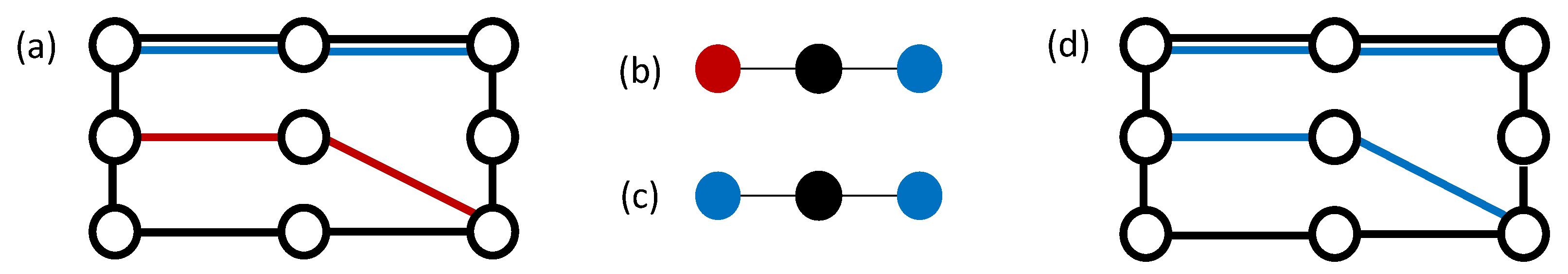
In more detail, consider a conflicts graph created using a single i-coloured vertex for each component of each subgraph $G^{*}\left(i\right)$ (for $i\in \{1,\dots ,k\}$), with edges corresponding to any vertex pair representing differently-coloured overlapping components in $G^{*}$. From a graph colouring perspective, note that the colours of the vertices in this conflicts graph define a proper k-colouring, in that pairs of adjacent vertices will always have different colours; however, it may be possible to colour this conflicts graph using fewer colours. If this is so, then an equivalent graph to G with fewer colours can also be created. An example of this process is shown in Figure 4. This illustrates that, while the number of different edge colours k could have any value up to and including m, the minimum number of colours needed to express this graph might well be smaller. However, identifying this minimum can be difficult since it is equivalent to solving the $\mathcal{NP}$-hard chromatic number (graph colouring) problem [26].

Given these observations on k, a better alternative for analysing complexity is to consider the number of colours entering and exiting each vertex (given by $|C^{-}\left(v\right)|$ and $|C^{+}\left(v\right)|$) and, in particular, their maximum values $c_{max}^{-}=max\{|C^{-}\left(v\right)|:v\in V\}$ and $c_{max}^{+}=max\{|C^{+}\left(v\right)|:v\in V\}$. These will be used in the next section.

4. Methods Avoiding Expansion

In this section we now propose two variants of Dijkstra’s algorithm. These are designed to find shortest paths in our edge-coloured graphs (that is, graphs featuring transfer penalties at their vertices), but without the need for first performing a graph expansion.

4.1. Extended Dijkstra Version 1

Our first adaptation, Extended-Dijkstra-V1, is given in Algorithm 3. The rationale for this method can be explained by considering a cluster of dummy vertices in a Kirby–Potts expanded graph. As previously noted, vertices in each cluster of the expanded graph can be partitioned into two sets: in-vertices and out-vertices (see Figure 3a,b). Moreover, observe that a shortest path from an in-vertex must always next pass through an out-vertex from the same cluster before moving to a different cluster. As proven in Theorem 1 below, it is therefore sufficient to simply add the length of the corresponding transfer (edge) to the path here, rather than consider the out-vertices as separate entities within the graph.

The idea in our approach is to therefore use a pair $(u,i)$ for each vertex $u\in V$ and incoming colour $i\in C^{-}\left(u\right)$, giving ${\sum }_{u\in V}|C^{-}\left(u\right)|$ pairs in total. The source is also defined by such a pair $(s,l)$, which is interpreted as meaning that the paths should start at $s\in V$, assuming initial entry to s on an edge of colour l. Similarly to the Dijkstra procedure of Algorithm 1, during execution this algorithm stores labels, predecessors and the distinguished status of each pair using the data structures L, P and D respectively. At termination, all pairs reachable from the source are marked as distinguished, and the label $L(u,i)$ holds the length of the shortest path from the source to vertex u, assuming entry at u on an edge of colour i.

An example solution from this method is shown in Figure 5. The main differences between this approach and Dijkstra are (a) the use of vertex-colour pairs, and (b) at Lines 11 and 13 of Extended-Dijkstra-V1, where transfer penalties $t(u,i,j)$ are added when comparing and recalculating label values. Note also that for $k=1$ this algorithm becomes equivalent to Dijkstra.

Algorithm 3 The extended Dijkstra algorithm, version 1.
	Extended-Dijkstra-V1 $(s\in V,l\in C^{-}\left(s\right))$
(1)	for all $v\in V$
(2)	for all $i\in C^{-}\left(v\right)$
(3)	Set $L(v,i)=\infty$; $D(v,i)=$ false; and $P(v,i)=$ null
(4)	Set $L(s,l)=0$ and $Q=\left\{\right(s,l,L(s,l)\left)\right\}$
(5)	while $Q\ne \varnothing$
(6)	Let $(u,i,x)$ be the element in Q with minimum value for x
(7)	Remove $(u,i,x)$ from Q and set $D(u,i)=$ true
(8)	for all $(u,v,j)\in E^{+}\left(u\right)$ such that $D(v,j)=$ false
(9)	if $L(u,i)+t(u,i,j)+w(u,v,j)<L(v,j)$ then
(10)	if $L(v,j)\ne \infty$ then remove $(v,j,L(v,j\left)\right)$ from Q
(11)	Set $L(v,j)=L(u,i)+t(u,i,j)+w(u,v,j)$; $P(v,j)=(u,i)$; and insert $(v,j,L(v,j\left)\right)$ into Q

The correctness of Extended-Dijkstra-V1 is due to the following theorem.

Theorem 1.

If all edge weights and transfer penalties in a graph are nonnegative then, for all distinguished pairs $(u,i)$, the label $L(u,i)$ is the length of the shortest path from the source $(s,l)$ to $(u,i)$.

Proof. 

Proof is by induction on the number of distinguished pairs. When there is just one distinguished pair, the theorem clearly holds since the length of the shortest path from $(s,l)$ to itself is $L(s,l)=0$.

For the step case, let $(v,j)$ be the next pair to be marked as distinguished by the algorithm (i.e., $L(v,j)$ is minimal among all undistinguished pairs) and let $(u,i)$ be its predecessor. Hence the shortest $(s,l)$-$(v,j)$-path has length $L(u,i)+t(u,i,j)+w(u,v,j)$. Now consider any other path P from $(s,l)$ to $(v,j)$. We need to show that the length of P cannot be less than $L(u,i)+t(u,i,j)+w(u,v,j)$. Let $(x,a)$ and $(y,b)$ be pairs on P such that $(x,a)$ is distinguished and $(y,b)$ is not, meaning that P contains the edge $(x,y,b)$. This implies that the length of P is greater than or equal to $L(x,a)+t(x,a,b)+w(x,y,b)$ (due to the induction hypothesis). Similarly, this figure must be greater than or equal to $L(u,i)+t(u,i,j)+w(u,v,j)$ because, as assumed, $L(v,j)$ is minimal among all undistinguished pairs. □

We now consider the computational complexity of Extended-Dijkstra-V1. As before, we assume the use of a binary heap for Q and direct access data structures for L, D and P. The initialisation of L, D, and P in Lines 1 to 5 has a worst-case complexity of $\mathcal{O}\left(n{c}_{\max }^{-}\right)$. For the main part of the algorithm, note that each label in L is considered and marked as distinguished exactly once and, in the worst case, we will have $n{c}_{\max }^{-}$ such labels. Once a label $(u,i)$ is marked as distinguished, all incident edges $(u,v,j)$ are then considered in turn and are subject to a series of constant-time and log-time operations, as shown in Lines 12 to 15. This leads to an overall worst case complexity of $\mathcal{O}\left(n{c}_{\max }^{-}\right)+\mathcal{O}\left(\left(m{c}_{\max }^{-}\right)lg\left(n{c}_{\max }^{-}\right)\right)$. Assuming graph connectivity, this simplifies to a growth rate for Extended-Dijkstra-V1 of

$$\begin{array}{ccc}\hfill f_1& =& \mathcal{O}\left(\left(m{c}_{\max }^{-}\right)lg\left(n{c}_{\max }^{-}\right)\right).\hfill \end{array}$$

(3)

As previously noted, the complexity of Dijkstra using a binary heap is $\mathcal{O}(mlgn)$. Using a Kirby–Potts expansion, in the worst case this leads to a graph $G^{\prime }$ with $n^{\prime }=n(c_{\max }^{-}+c_{\max }^{+})$ vertices and $m^{\prime }=m+n{c}_{\max }^{-}{c}_{\max }^{+}$ edges, giving an overall complexity of $\mathcal{O}(m^{\prime }lg{n}^{\prime })$, or

$$\begin{array}{ccc}\hfill f_2& =& \mathcal{O}\left(\left(m+n{c}_{\max }^{-}{c}_{\max }^{+}\right)lg\left(n\left(c_{\max }^{-}+c_{\max }^{+}\right)\right)\right).\hfill \end{array}$$

(4)

Figure 6 compares $f_1$ and $f_2$ for a range of different parameter values. Note that $f_1$ grows more quickly in all cases, demonstrating that Extended-Dijkstra-V1 is less efficient with regards to increases in the number of edges m. The main reason for this is that, with Extended-Dijkstra-V1, each outgoing edge of a vertex v is considered for each incoming colour of v. This results in the term $\left(m{c}_{\max }^{-}\right)$ seen in Equation (3). In contrast, although a Kirby–Potts expansion results in a graph $G^{\prime }$ with an increased number of edges and vertices, each edge in $G^{\prime }$ is considered only once using Dijkstra, which results in a slower growth rate. Note, however, that each chart in Figure 6 features an intersect, suggesting that Extended-Dijkstra-V1 is more efficient with very sparse graphs. (If Fibonacci heaps are used for Q instead of binary heaps, the growth rates for $f_1$ and $f_2$ are $\mathcal{O}(\left(m{c}_{\max }^{-}\right)+\left(n{c}_{\max }^{-}\right)lg\left(n{c}_{\max }^{-}\right))$ and $\mathcal{O}(m^{\prime }+n^{\prime }lg{n}^{\prime })$ respectively. These feature the same noted properties as $f_1$ and $f_2$ except that growth is more gradual, and intersects occur at slightly higher values of m.) For indicative purposes, the grey rectangles in the figure show the range of values for which planar digraphs exist (i.e., the right boundary of these rectangles occur at $m=2(3n-6)$, which is the maximum possible number of directed edges in a planar digraph). Planar graphs are considered further in Section 5.

4.2. Extended Dijkstra Version 2

Our second adaptation operates by replicating the behaviour of Dijkstra’s algorithm on Kirby–Potts graphs. This results in a method with the more favourable growth rate of $f_2$ but that also avoids the need for graph expansion. To do this, approximately twice as much working memory as Extended-Dijkstra-V1 is required because, in addition to storing values for each vertex/in-colour pair, we also need to store values for each vertex/out-colour pair. The structures L, D and P are therefore replaced with the structures $L_{\mathrm{in}}$ and $L_{\mathrm{out}}$, $D_{\mathrm{in}}$ and $D_{\mathrm{out}}$, and $P_{\mathrm{in}}$ and $P_{\mathrm{out}}$.

The complete procedure for Extended-Dijkstra-V2 is given in Algorithm 4. Note that each item in the priority queue Q is now a tuple comprising four values. The fourth value indicates whether the item refers to an “in-label” or and “out-label”, which correspond to in-vertices and out-vertices in a Kirby–Potts graph. The item $(u,i,x,\mathrm{IN})\in Q$ means that we are considering the vertex u, incoming edges of colour i, and that $L_{\mathrm{in}}(u,i)=x$. Similarly, $(u,i,x,\mathrm{OUT})\in Q$ means we are considering vertex u, outgoing edges of colour i, and that $L_{\mathrm{out}}(u,i)=x$.

Algorithm 4 The extended Dijkstra algorithm, version 2.
	Extended-Dijkstra-V2 $(s\in V,l\in C^{-}\left(s\right))$
(1)	for all $v\in V$
(2)	for all $i\in C^{-}\left(v\right)$
(3)	Set $L_{\mathrm{in}}(v,i)=\infty$; $D_{\mathrm{in}}(v,i)=$ false; and $P_{\mathrm{in}}(v,i)=$ null
(4)	for all $i\in C^{+}\left(v\right)$
(5)	Set $L_{\mathrm{out}}(v,i)=\infty$; $D_{\mathrm{out}}(v,i)=$ false; and $P_{\mathrm{out}}(v,i)=$ null
(6)	Set $L_{\mathrm{in}}(s,l)=0$ and $Q=\left\{(s,l,L_{\mathbf{in}}(s,l),\mathrm{IN})\right\}$
(7)	while $Q\ne \varnothing$
(8)	Let $(u,i,x,y)$ be the element in Q with minimum value for x
(9)	Remove $(u,i,x,y)$ from Q
(10)	if $(y=\mathrm{IN})$ then
(11)	Set $D_{\mathrm{in}}(u,i)=$ true
(12)	for all $j\in C^{+}\left(u\right)$ such that $D_{\mathrm{out}}(u,j)=$ false
(13)	if $L_{\mathrm{in}}(u,i)+t(u,i,j)<L_{\mathrm{out}}(u,j)$ then
(14)	if $L_{\mathrm{out}}(u,j)\ne \infty$ then remove $(u,j,L_{\mathrm{out}}(u,j),\mathrm{OUT})$ from Q
(15)	Set $L_{\mathrm{out}}(u,j)=L_{\mathrm{in}}(u,i)+t(u,i,j)$; $P_{\mathrm{out}}(u,j)=(u,i)$; and insert $(u,j,L_{\mathrm{out}}(u,j),\mathrm{OUT})$ into Q
(16)	else
(17)	Set $D_{\mathrm{out}}(u,i)=$ true
(18)	for all $(u,v,j)\in E^{+}\left(u\right)$ such that $j=i$ and $D_{\mathrm{in}}(v,i)=$ false
(19)	if $L_{\mathrm{out}}(u,i)+w(u,v,i)<L_{\mathrm{in}}(v,i)$ then
(20)	if $L_{\mathrm{in}}(v,i)\ne \infty$ then remove $(v,i,L_{\mathrm{in}}(v,i),\mathrm{IN})$ from Q
(21)	Set $L_{\mathrm{in}}(v,i)=L_{\mathrm{out}}(u,i)+w(u,v,i)$; $P_{\mathrm{in}}(v,i)=(u,i)$; and insert $(v,i,L_{\mathrm{in}}(v,i),\mathrm{IN})\}$ into Q

As shown in Algorithm 4, items are selected and removed from the priority queue Q on Lines 8 and 9. If the selected item $(u,i,x,y)$ refers to an in-label ($y=\mathrm{IN}$), then only labels referring to the outgoing colours of vertex u need to be considered for update; hence, we only need to look at the transfer penalties $t(u,i,j)$ for $j\in C^{+}\left(u\right)$ in which $D_{\mathrm{out}}(u,j)$ is not distinguished (Lines 12 to 15). Similarly, if $(u,i,x,y)$ refers to an out-label ($y=\mathrm{OUT}$), then we only need to consider updating the in-labels of any vertex v connected to u by an edge of colour i (Lines 18 to 21). This behaviour is identical to the way in which Dijkstra would operate with a Kirby–Potts expanded version of the graph.

5. Computational Comparison

In this section we consider the CPU times required to calculate shortest path trees on various types of edge-coloured graphs. In particular, we wish to assess the relative performances of our extended Dijkstra methods in comparison to using Dijkstra’s original algorithm on Kirby–Potts expanded graphs. Note that we do not include the time taken to perform Kirby–Potts expansions in these results. This is because the decision on how a graph is represented and stored will often be made by the user beforehand and might therefore be considered a separate process. However, this will not always be the case as we discuss in Section 5.4.

In our experiments, we will seek shortest paths in which transfer penalties are not incurred at terminal vertices. This is useful in applications such as public transport, where a passenger will arrive at the source vertex by means outside of the network (e.g., by foot), and will then leave the network on arrival at their destination. To make this modification on an edge-coloured graph we can simply set all transfer penalties at the source vertex s to zero before running the shortest path algorithm using an arbitrary in-colour $l\in C^{-}\left(s\right)$ (in cases where the source vertex s does not feature an in-colour ($C^{-}\left(s\right)=\varnothing$), then a dummy in-colour can be temporarily added to the graph.). The length of the shortest s-v-path in G is then indicated by the minimum value among the labels of v. For a Kirby–Potts expanded graph $G^{\prime }$, a similar process is used: first, the weights of all transfer edges in the cluster defined by s are temporarily set to zero; next Dijkstra is executed from an arbitrary in-vertex within this cluster; finally, the minimum label value among all in-vertices in v’s cluster is identified.

Three types of problem instances are considered in our tests: random graphs, planar graphs, and real-world public transport networks. The latter are considered in more detail in Section 5.3. Our random graphs were generated by randomly placing n vertices into the unit square. All potential edges $(u,v,i)$ were then considered in turn and added to the graph with a fixed probability of $d/k$, where d is a density parameter representing the average number of edges travelling from each vertex u to each vertex v. During this process, care was also taken to ensure that the graph contained a random $(n-1)$-cycle, making the graph strongly connected.

The second graph type, planar graphs, were considered to give a general indication of algorithm performance on transport networks. Recall that planar graphs are those that can be drawn on a plane so that no edges cross. In that sense, like road networks, they are quite sparse, with vertex degrees being fairly low. Note that when things like roads physically intersect on land, there will often be an opportunity to transfer from one to the other; hence, the underlying graph will be planar. However, this is not always the case, such as when one road crosses another via a bridge, so the analogy is not exact. Planar graphs were formed by again randomly placing n vertices into the unit square. A Delaunay triangulation was then generated from these vertices, with the edges of this triangulation being used to form a pool of potential edges for the graph (that is, for each edge $\{u,v\}$ in the triangulation, all directed and coloured edges $(u,v,i)$ and $(v,u,i)$ (for $i\in \{1,\dots ,k\}$) were added to the pool). Edges were then selected randomly from this pool and added to the graph until the desired graph density was reached. Again, we also ensured that the resultant graph was strongly connected: in this case by including all edges from a bidirectional minimum spanning tree.

For both random and planar graphs, edge weights were calculated using the Euclidean distances between vertices plus x per cent where, for each edge, x was selected randomly in the range $(-10,10)$. This prevents edges between the same pair of vertices from having the same weight. Transfer penalties were set to the average edge weight across the graph plus or minus x per cent.

Our algorithm implementations were written in C++ and executed on 3.2 GHtz Windows 7 machines with 8 GB RAM. In all implementations, C++ sets (red-black trees) were used for the priority queues and C++ unordered maps (hash tables) were used for storing transfer penalties $t(u,i,j)$. Graphs were represented using an array of adjacency lists, one list for each vertex. For a vertex v, lists were then stored using C++ sets. Each item in a list then contained the label of a neighbouring vertex, together with the colour and weight of the corresponding edge. For Extended-Dijkstra-V2, which requires access to neighbours only joined by a specific edge colour, adjacency lists were maintained for each vertex/colour pair. All source code and results are available online at [27].

5.1. Random Graphs

Figure 7 shows the average CPU times of our implementations using random graphs with $n\in \{100,1000,10000\}$ and $k\in \{3,10,20\}$. In all cases, five graphs were generated for each density $d\in \{0,0.02,0.04,\dots ,1.0\}$ and algorithms were run using each of the n vertices as a source in turn. Each point in the figure is therefore a mean of $5n$ different values. As an additional means of comparison, we also ran a second (slightly slower) implementation of Dijkstra’s algorithm on Kirby–Potts expanded graphs, available in the Python package NetworkX (v. 2.4).

As might be expected, Figure 7 shows that run times grow for increases in n, m, and k. In general we see that using Dijkstra’s algorithm with Kirby–Potts graphs gives the shortest run times, with Extended-Dijkstra-V2 a close second. The differences in these two algorithms seems due to our choice of data structures. As noted, in Kirby–Potts graphs all information is encoded via adjacency lists hence, during execution, Dijkstra’s algorithm is able to access this information directly when iterating through each list. When using Extended-Dijkstra-V2, on the other hand, the overheads involved in using hash tables for storing the transfer penalties makes accessing each value of $t(u,i,j)$ slightly more expensive. (Indeed, in preliminary tests we found that our implementation of Extended-Dijkstra-V2 could be improved for small instances by using a different data structure. This was achieved by maintaining an $n\times k\times k$ array in which an element $(u,i,j)$ referred to $t(u,i,j)$. However, in many problem instances this array wasted a lot of space because transfers between various pairs of colours did not exist at vertices. For some of the larger real-world problem instances used in Section 5.3, for example, the memory requirements of this array exceeded 40 GB.)

Figure 7 also shows that the gap in the time requirements of Extended-Dijkstra-V1 compared to Kirby–Potts and Extended-Dijkstra-V2 widens for increases in n, k, and m. Indeed, the most extreme difference occurs with graphs with $n=10,000$, $d=1.0$, and $k=20$, where a difference of over twenty seconds per shortest-path tree is observed. That said, the effects of the asymptotic growth rate intersections (as seen in Figure 6) are also apparent with small sparse graphs, where Extended-Dijkstra-V1 has slightly shorter running times.

5.2. Planar Graphs

Figure 8 shows the average CPU times required by our implementations with planar graphs. Here, for each n and k, graphs were generated for twenty-five different values for m, using an upper limit of $m=2k(3n-6)$ (this is the maximum number of edges in a planar, loop-free, multi-digraph using k edge colours). As with Figure 6, the right boundaries of the grey rectangles in these charts indicate $m=2(3n-6)$ (the maximum number of edges in a planar digraph). All other experimental details are the same as the previous subsection.

Figure 8 reveals similar patterns to those seen for random graphs, with time requirements growing for increases in n, m, and k with all algorithms. In this case, however, the relative sparsity of planar graphs allows us to view areas in which Extended-Dijkstra-V1 has the shortest run times. However, as previously seen in Figure 6, increases in the number of edges eventually leads to an intersect, with Kirby–Potts then showing the most favourable run times overall.

5.3. Public Transport Graphs

We now consider the relative performance of our implementations on real-world public transport networks. In these graphs, vertices represent access points (stations, bus stops, etc.) and edges represent connection times between adjacent pairs. The first of these is the London Underground network and includes 302 stations and thirteen different transport lines [28]. The remainder are due to Kujala et al. [29] who have gathered public transport information from 27 different cities. For each city in their set, information about all forms of public transport is given, including trains, buses, trams and ferries. In our case, a different colour was used for each route of each mode, and transfer times were determined in the same way as our random and planar graphs.

A summary of these 28 problem instances is given in

Table 2. Summary of the 28 real-world problem instances. In columns indicating the number of edges m, daggers (†) indicate strongly connected graphs. For instances with 1 km walks, an extra edge colour is required, meaning that k and $\overline{\chi }$ should be incremented by one. The meaning of the asterisks (*) is described in the text.

City	Original Instances (No Walking)						With 1 km Walks
	$\mathit{n}$	$\mathit{k}$	${\mathit{c}}_{\mathbf{max}}^{-}$	${\mathit{c}}_{\mathbf{max}}^{+}$	$\overline{\mathit{\chi }}$	$\mathit{m}$	$\mathit{m}$
London Underground	302	13	6	6	9 *	812 ${}^{†}$	812 ${}^{†}$
Kuopio	549	33	13	13	18 *	1626	10,436
Antofagasta	650	17	14	14	16 *	2547	26,291 ${}^{†}$
Luxembourg	1367	222	59	59	77 *	6163	18,153 ${}^{†}$
Rennes	1407	50	7	7	8 *	2159	29,219 ${}^{†}$
Grenoble	1547	52	4	4	5 *	1943	37,529 ${}^{†}$
Turku	1850	103	35	35	35 *	7080	54,230
Venice	1874	873	90	90	90 *	16,561	42,983
Belfast	1917	102	31	27	31 *	6041	64,635 ${}^{†}$
Palermo	2176	94	17	17	17 *	5298 ${}^{†}$	91,962 ${}^{†}$
Nantes	2353	97	9	8	9 *	4080	58,130
Canberra	2764	123	35	35	38	7121	57,687 ${}^{†}$
Toulouse	3329	104	9	9	9 *	5067	78,557 ${}^{†}$
Bordeaux	3435	81	8	8	9 *	5829	91,087 ${}^{†}$
Dublin	4571	143	23	23	25	12,165	132,729
Berlin	4601	575	59	59	60	22,922	59,108
Winnipeg	5079	90	33	33	40 *	10,642	211,124 ${}^{†}$
Prague	5147	356	21	21	24 *	14,807	90,035
Detroit	5683	40	8	8	8 *	6460	195,584 ${}^{†}$
Athens	6768	240	18	18	18 *	14,741	259,923 ${}^{†}$
Helsinki	6986	498	64	64	64 *	27,718	223,382
Lisbon	7073	868	32	29	33 *	23,354	243,792 ${}^{†}$
Adelaide	7548	517	82	82	82 *	32,018	197,062 ${}^{†}$
Rome	7869	337	17	17	18 *	19,164	287,964
Brisbane	9645	401	60	60	60 *	20,849	249,537
Paris	11,950	878	10	10	11	20,810	511,248 ${}^{†}$
Melbourne	19,493	405	18	18	18 *	28,738	498,084
Sydney	24,063	736	42	42	50	55,616	714,902

. As shown, they range in size from $n=302$ to $24,063$, with values of k between 13 and 868. Note that a small amount of cleaning was required with Kujala et al.’s instances to eliminate loops and edges with undefined endpoints. In addition, many of the instances do not form strongly connected components, meaning that paths are not available between all pairs of access points. (That said, we found that more than 95% of access points are contained within one large strongly connected component in all cases.) As a result, we also created a secondary version of Kujala et al.’s instances in which walks of up to 1 km are permitted between access points using an average walking speed of 1.4 metres per second. As shown this increases the number of edges in the graphs, though some networks still remain disconnected. Illustrations of two networks are given in Figure 9.

Finally, Table 2 also contains information on the minimum number of colours $\overline{\chi }$ needed to represent these graphs, as explained in Section 3.3. In all cases $\overline{\chi }$ is less than k; quite drastically so with some of the larger instances such as Paris, Melbourne and Sydney. These figures were gained by converting the transport networks into conflicts graphs and then running a backtracking version of the DSatur heuristic for graph colouring for a maximum of one hour per instance [26,30]. Asterisks in Table 2 indicate the proven minimum number of colours for these graphs (the chromatic number). All other figures are upper bounds on this number.

The charts in Figure 10 summarise the results with these instances. In the majority of cases, the use of Dijkstra’s algorithm with Kirby–Potts graphs gives the shortest average run times. Run times of our extended algorithms are therefore stated as a proportion of these times. (A proportion increase of one indicates a 100% increase in run time). As shown, when walks between access points are not included in the graphs, their relative sparsity allows Extended-Dijkstra-V1 to execute run more quickly than V2 in nearly all cases. However, once walks of up to 1 km are included, the increased density sees V2 running more quickly.

5.4. Expansion Times

As previously noted, our experiments to this point have not included the time taken to perform Kirby–Potts expansions. However, there are some cases where this issue is quite important. For example, Ahmed et al. [20] and Heyken Soares et al. [23] have proposed methods for optimising public transport systems that use heuristics to produce a whole series of graphs, each that must then be expanded before evaluation. In these cases, it therefore seems more appropriate to consider the overheads consumed by these expansions.

In our case, an expansion takes a graph G and produces a corresponding adjacency list for the expanded graph $G^{\prime }$. This involves stepping through each edge and transfer penalty in G and then adding an appropriate edge to $G^{\prime }$. This leads to an overall complexity of $\mathcal{O}(m+n{c}_{\max }^{-}{c}_{\max }^{+})$. Note that this has a slightly lower growth rate compared to executing Dijkstra on $G^{\prime }$, shown in Equation (4).

Table 3. Number of seconds to perform Kirby-Potts expansions for random and planar graphs of differing parameters. Figures show the mean and standard deviation across twenty problem instances.

Random Graphs			Planar Graphs
	Conversion Time			Conversion Time
Parameters	Mean	Std. dev.	Parameters	Mean	Std. dev.
$n=1000$:			$n=1000$:
$d=0.05$, $k=3$	$0.006$	<0.001	$m=1998$, $k=3$	<0.001	$0.001$
$d=0.50$, $k=3$	$0.058$	$0.002$	$m=9661$, $k=3$	$0.003$	$0.001$
$d=0.95$, $k=3$	$0.113$	$0.001$	$m=17,325$, $k=3$	$0.003$	<0.001
$d=0.05$, $k=10$	$0.017$	<0.001	$m=1998$, $k=10$	$0.001$	<0.001
$d=0.50$, $k=10$	$0.063$	$0.001$	$m=29,781$, $k=10$	$0.016$	$0.002$
$d=0.95$, $k=10$	$0.113$	$0.001$	$m=57,564$, $k=10$	$0.017$	$0.001$
$d=0.05$, $k=20$	$0.055$	$0.001$	$m=1998$, $k=20$	$0.001$	$0.001$
$d=0.50$, $k=20$	$0.108$	$0.002$	$m=58,523$, $k=20$	$0.059$	$0.002$
$d=0.95$, $k=20$	$0.162$	$0.016$	$m=115,049$, $k=20$	$0.068$	$0.004$
$n=10,000$:			$n=10,000$:
$d=0.05$, $k=3$	$0.602$	$0.006$	$m=19,998$, $k=3$	$0.008$	<0.001
$d=0.50$, $k=3$	$6.640$	$0.161$	$m=96,781$, $k=3$	$0.028$	$0.001$
$d=0.95$, $k=3$	$38.369$	$6.452$	$m=173,565$, $k=3$	$0.034$	$0.001$
$d=0.05$, $k=10$	$0.714$	$0.004$	$m=19,998$, $k=10$	$0.009$	$0.001$
$d=0.50$, $k=10$	$6.550$	$0.229$	$m=298,341$, $k=10$	$0.203$	$0.006$
$d=0.95$, $k=10$	$44.437$	$8.754$	$m=576,684$, $k=10$	$0.232$	$0.008$
$d=0.05$, $k=20$	$1.193$	$0.014$	$m=19,998$, $k=20$	$0.010$	$0.001$
$d=0.50$, $k=20$	$6.768$	$0.092$	$m=586,283$, $k=20$	$0.689$	$0.002$
$d=0.95$, $k=20$	$53.360$	$7.904$	$m=1,152,569$, $k=20$	$0.770$	$0.016$

shows the conversion times for random and planar graphs of differing parameters. We see that these times increase for graphs featuring more edges, vertices, and colours. For graphs with $n=1000$, conversion times are very small, coming in at less than 0.2 s in all cases; however, for larger graphs much longer times are sometimes required. Note that the largest Kirby–Potts graphs seen here (produced from random graphs with $n=10,000$, $d=0.95$ and $k=20$) required over 5 GB of RAM, and so significant amounts of memory management were also needed as part of this expansion process.

6. Conclusions

This paper has proposed two new shortest path algorithms that are able to handle vertex transfer penalties without first having to perform a graph expansion. Our first method, Extended-Dijkstra-V1, exhibits an inferior growth rate compared to using Dijkstra’s algorithm on Kirby–Potts graphs; however, it has the potential to exhibit shorter run times with very sparse problem instances such as planar graphs. In contrast, our second variant Extended-Dijkstra-V2 has the same growth rate as Dijkstra’s algorithm with Kirby–Potts graphs, though in our implementations its run times do seem to be marginally higher.

During our research, we also experimented with a modified version of Extended-Dijkstra-V1 in which, when a label $(u,i)$ was marked as distinguished, all incoming edges at u with colour i were removed. The intention behind this modification was to prevent these edges from being considered more than once during the run and therefore help to improve run times. However, this method was significantly slower for two reasons: first, because a copy of the graph had to be made before each application of the algorithm; second, because of the additional costs involved in seeking and removing edges from the adjacency lists.

Note that in this paper we have considered graphs in which transfer penalties $t(u,i,j)\in T$ are static. In applications such as public transport, however, transfer penalties may also depend on the time of arrival at a vertex and the subsequent scheduled time of departure (consider trains that leave stations according to a timetabled service, for example). Previous work due to Cooke and Halsey [31] and Dreyfus [32] has shown that Dijkstra’s algorithm is suitable in these time-dependent scenarios providing that the “first-in first-out” (FIFO) property is met. This simply states that, on every edge $(u,v,i)\in E$, an earlier departure from u will lead to an earlier arrival at v, while a later departure from u will lead to a later arrival at v. The FIFO property is met when calculating departure times based on scheduled services; however, shortest path problems on non-FIFO graphs are known to be $\mathcal{NP}$-hard in general [33].

In future work it would also be interesting to determine whether other shortest-path algorithms can be modified for graphs featuring vertex transfer penalties. For instance, a similar extension to the A* algorithm may prove to be useful for the single-source single-target shortest path problem. This would involve devising an admissible heuristic rule for selecting items from the priority queue.

References

- Mills, B. Theoretical Introduction to Programming; Springer: London, UK, 2005. [Google Scholar]
- Six Degrees of Separation. 2020. Available online: https://en.wikipedia.org/wiki/Six_degrees_of_separation (accessed on 19 July 2020).
- Lewis, R. Who is the Centre of the Movie Universe? Using Python and NetworkX to Analyse the Social Network of Movie Stars. arXiv 2020, arXiv:2002.11103. [Google Scholar]
- Sedgewick, R. Algorithms in Java, Part 5: Graph Algorithms, 3rd ed.; AddisonWesley Professional: Boston, MA, USA, 2003. [Google Scholar]
- Cormen, T.; Leiserson, C.; Rivest, R.; Stein, C. Introduction to Algorithms, 3rd ed.; The MIT Press: Cambridge, MA, USA, 2009. [Google Scholar]
- Dijkstra, E. A Note on Two Problems in Connexion with Graphs. Numer. Math. 1959, 1, 269–271. [Google Scholar] [CrossRef] [Green Version]
- Frana, P. An Interview with Edsger W. Dijkstra. Commun. ACM 2010, 53, 41–47. [Google Scholar] [CrossRef]
- Bauer, R.; Delling, D.; Sanders, P.; Schieferdecker, D.; Schultes, D.; Wagner, D. Combining Hierarchical and Goal-Directed Speed-Up Techniques for Dijkstra’s Algorithm. In Experimental Algorithms; McGeoch, C., Ed.; Springer: Berlin/Heidelberg, Germany, 2008; Volume 5038, pp. 303–318. [Google Scholar]
- Moore, F. The Shortest Path through a Maze; Technical Report; Bell Telephone System, USA: Boston, MA, USA, 1959; Volume 3523. [Google Scholar]
- Ahuja, R.; Mehlhorn, K.; Orlin, J.; Tarjan, R. Faster Algorithms for the Shortest Path Problem. J. ACM 1990, 37, 213–223. [Google Scholar] [CrossRef] [Green Version]
- Gabow, H.; Tarjan, R. Faster Scaling Algorithms for Network Problems. SIAM J. Comput. 1989, 18, 1013–1036. [Google Scholar] [CrossRef] [Green Version]
- Johnson, D. Efficient Algorithms for Shortest Paths in Sparse Networks. J. ACM 1977, 24, 1–13. [Google Scholar] [CrossRef]
- Hart, P.; Nilsson, N.; Raphael, B. A Formal Basis for the Heuristic Determination of Minimum Cost Paths. IEEE Trans. Syst. Sci. Cybern. 1968, 4, 100–107. [Google Scholar] [CrossRef]
- Hart, P.; Nilsson, N.; Raphael, B. Correction to ‘A Formal Basis for the Heuristic Determination of Minimum Cost Paths’. ACM SIGART Bull. 1972, 37, 28–29. [Google Scholar] [CrossRef]
- Fu, L.; Sun, D.; Rilett, L. Heuristic Shortest Path Algorithms for Transportation Applications: State of the Art. Comput. Oper. Res. 2006, 33, 3324–3343. [Google Scholar] [CrossRef]
- Yen, J. Finding the k Shortest Loopless Paths in a Network. Manag. Sci. 1971, 17, 712–716. [Google Scholar] [CrossRef]
- Bhandari, R. Survivable Networks: Algorithms for Diverse Routing; Kluwer Academic Publishers: Norwell, MA, USA, 1999. [Google Scholar]
- Demir, E.; Burgholzer, W.; Hrusovsky, M.; Arikan, E.; Jammernegg, W.; Van Woensel, T. A Green Intermodal Service Network Design Problem with Travel Time Uncertainty. Transp. Res. Part B 2016, 93, 789–807. [Google Scholar] [CrossRef]
- Kirby, R.; Potts, R. The Minimum Route Problem for Networks with Turn Penalties and Prohibitions. Transp. Res. 1969, 3, 397–408. [Google Scholar] [CrossRef]
- Ahmed, L.; Mumford, C.; Kheiri, A. Soving Urban Transit Route Design Problems using Selection Hyper-heuristics. Eur. J. Oper. Res. 2019, 274, 545–559. [Google Scholar] [CrossRef]
- Cooper, I.; John, M.; Lewis, R.; Mumford, C.; Olden, A. Optimising Large Scale Public Transport Network Design Problems using Mixed-mode Parallel Multi-objective Evolutionary Algorithms. In Proceedings of the 2014 IEEE Congress on Evolutionary Computation, Beijing, China, 6–11 July 2014; pp. 2841–2848. [Google Scholar]
- John, M. Metaheuristics for Designing Efficient Routes and Schedules for Urban Transportation Networks. Ph.D. Thesis, School of Computer Science and Informatics, Cardiff University, Cardiff, UK, 2016. [Google Scholar]
- Heyken Soares, P.; Mumford, C.; Amponsah, K.; Mao, Y. An Adaptive Scaled Network for Public Transport Route Optimisation. Public Transp. 2019, 11, 379–412. [Google Scholar] [CrossRef] [Green Version]
- John, M.; Mumford, C.; Lewis, R. An Improved Multi-objective Algorithm for the Urban Transit Routing Problem. In Evolutionary Computation in Combinatorial Optimisation; Springer: Berlin, Germany, 2014; Volume 8600, pp. 49–60. [Google Scholar]
- Winter, S. Modeling Costs of Turns in Route Planning. GeoInformatica 2002, 6, 345–361. [Google Scholar] [CrossRef]
- Lewis, R. A Guide to Graph Colouring: Algorithms and Applications; Springer International Publishing: Cham, Switzerland, 2016. [Google Scholar] [CrossRef]
- Source Code and Results Tables. Available online: http://www.rhydlewis.eu/resources/spalgs.zip (accessed on 1 October 2020).
- Greco, N. London Underground Dataset. Available online: https://github.com/nicola/tubemaps (accessed on 15 July 2020).
- Kujala, R.; Weckstrom, C.; Darst, R.; Mladenovic, M.; Saramaki, J. A Collection of Public Transport Network Data Sets for 25 Cities. Sci. Data 2018. Available online: http://transportnetworks.cs.aalto.fi/ (accessed on 21 October 2020). [CrossRef] [PubMed] [Green Version]
- Brélaz, D. New Methods to Color the Vertices of a Graph. Commun. ACM 1979, 22, 251–256. [Google Scholar] [CrossRef]
- Cooke, K.; Halsey, E. The Shortest Route through a Network with Time-Dependent Internodal Transit Times. J. Math. Anal. Appl. 1966, 14, 493–498. [Google Scholar] [CrossRef] [Green Version]
- Dreyfus, S. An Appraisal of Some Shortest Path Algorithms. Oper. Res. 1969, 13, 395–412. [Google Scholar] [CrossRef]
- Orda, A.; Rom, R. Shortest-Path and Minimum-Delay Algorithms in Networks with Time-Dependent Edge-Length. J. ACM 1990, 37, 607–625. [Google Scholar] [CrossRef] [Green Version]
Figure 1.
An example graph with vertices. In this case, edges are drawn with straight lines and edge weights correspond to the lengths of these lines. This graph is also symmetric in that if and only if , with . The (left) figure shows a solution to the “single-source single-target” problem, where the source s is at the bottom-left and the target t is at top right. The (right) figure shows a solution to the “single source” problem—a shortest-path tree rooted at s.
Figure 2.
A small network comprising vertices, edges and colours. As per Definition 1 we have, for example, , , and .
Figure 3.
(a) The graph formed from Figure 2 using the Kirby–Potts expansion method; (b) an example cluster of dummy vertices produced using the Kirby–Potts method; and (c) the corresponding cluster using the (problematic) restricted expansion method.
Figure 4.
(a) A graph using colours; (b) the underlying conflicts graph (and 3-colouring) prescribed by ; (c) a 2-colouring of this conflicts graph; and (d) the original graph using colours.
Figure 5.
Solution returned by Extended-Dijkstra-V1 using the graph from Figure 2 and source . All transfer penalties are assumed to be 1. The shortest path tree rooted at is defined by the contents of P and is illustrated on the right.
Figure 6.
Comparison of growth rates and with regards to the number of edges m. Rows show n-values of 100, 1000 and 10,000 respectively; columns consider values of 3, 10, and 20 respectively.
Figure 7.
CPU times required to produce a shortest path tree from a single source using random graphs of differing densities. Rows show n values of 100, 1000 and 10,000 respectively; columns consider k-values of 3, 10 and 20 respectively. The number of edges in a graph is determined by multiplying the density by .
Figure 8.
CPU times required to produce a shortest path tree from a single source using planar graphs of differing densities. Rows show n values of 100, 1000 and 10,000 respectively; columns consider k-values of 3, 10 and 20 respectively. Note that results for NetworkX are not displayed in some charts because their CPU times exceed the chosen vertical scales.
Figure 9.
Public transport networks for the London Underground (left), and the city of Winnipeg (right). Vertices are positioned according to GPS coordinates.
Figure 10.
Comparison of run times for the real-world problem instances allowing no walks (top), and walks of up to 1 km (bottom).