CNN Based on Transfer Learning Models Using Data Augmentation and Transformation for Detection of Concrete Crack

Abstract

Cracks in concrete cause initial structural damage to civil infrastructures such as buildings, bridges, and highways, which in turn causes further damage and is thus regarded as a serious safety concern. Early detection of it can assist in preventing further damage and can enable safety in advance by avoiding any possible accident caused while using those infrastructures. Machine learning-based detection is gaining favor over time-consuming classical detection approaches that can only fulfill the objective of early detection. To identify concrete surface cracks from images, this research developed a transfer learning approach (TL) based on Convolutional Neural Networks (CNN). This work employs the transfer learning strategy by leveraging four existing deep learning (DL) models named VGG16, ResNet18, DenseNet161, and AlexNet with pre-trained (trained on ImageNet) weights. To validate the performance of each model, four performance indicators are used: accuracy, recall, precision, and F1-score. Using the publicly available CCIC dataset, the suggested technique on AlexNet outperforms existing models with a testing accuracy of $99.90\%$, precision of $99.92\%$, recall of $99.80\%$, and F1-score of $99.86\%$ for crack class. Our approach is further validated by using an external dataset, BWCI, available on Kaggle. Using BWCI, models VGG16, ResNet18, DenseNet161, and AlexNet achieved the accuracy of $99.90\%$, $99.60\%$, $99.80\%$, and $99.90\%$ respectively. This proposed transfer learning-based method, which is based on the CNN method, is demonstrated to be more effective at detecting cracks in concrete structures and is also applicable to other detection tasks.

1. Introduction

Concrete cracks are a common indication of concrete defects in civil engineering structures. It affects structural health and induces an additional risk of unexpected breakdowns and accidents [1,2]. Hence, detecting cracks regularly and taking appropriate actions for the safety of the concrete structure is of great significance. The traditional method of detecting cracks on concrete structures relies on professional observation. Such conventional methods are not only costly but also laborious, time-consuming, and on many occasions, dangerous too [3]. However, the recent advancement of machine learning-based image processing technologies has gained attention as an efficient and automated method to detect cracks on concrete structures that also overcome the cons of manual methods [4].

The growing computer vision community working on different image-detection methods. It has proposed many techniques over the decades, including thresholding [5], edge detection [6], and wavelet transforms [7], to name a few, where some of these methods address concrete crack detection problems. However, this field needs an efficient and reliable solution as the concrete images are challenged with various surface textures, irregularity of cracks, and background complexity that differs crack detection from other image analysis applications.

Recently, deep learning-based models, predominantly neural networks with multiple layers, are playing a significantly successful role in feature learning [8]. On top of that, the availability of high-performing computing facilities and ongoing improvement of excellent training methods on available datasets drive the rapid development of deep learning. In this saga, the convolutional neural network (CNN) is a feed-forward neural network that performs excellently in large-scale image processing [9,10]. Although some of these models proved excellent in feature extractions on different applications, their accuracy requires improvement for concrete crack detection. To achieve efficient performance, reduce training time, and overcome the lack of a humongous dataset, in this paper, we have proposed a method of transfer learning-based CNN with the pre-trained model that shows significant improvement [11]. Our work has made the following contribution:

• We conduct experiments on the CCIC dataset with four different CNN models (VGG16, ResNet18, DenseNet161, and AlexNet), applying the transfer learning technique for detecting concrete surface cracks from images and examination with other models to demonstrate the success of the suggested model.
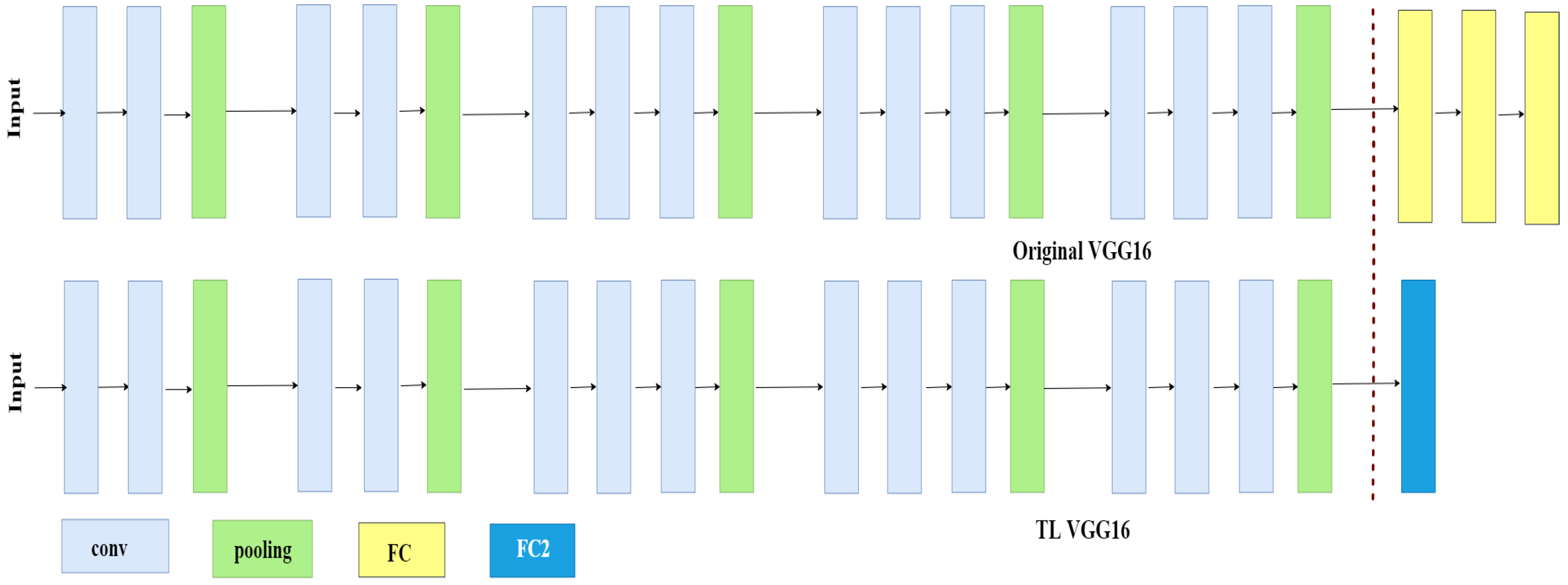
• We designed our model such that every CNN model has only one fully connected (FC) layer, having two output features for binary classification. We modified the VGG16 and AlexNet models by replacing the last three FC layers with only one FC layer.
• Our strategy is the most compatible with AlexNet, and it outperforms the competition. AlexNet achieves $99.90\%$ accuracy on the validation set on the CCIC dataset.
• The proposed method demonstrates superior crack detection for concrete structures, which can efficiently be utilized for other detection purposes.

The paper is now organized as follows. We provided a brief review of the literature in Section 2. Section 3 includes methodology, which describes experimental Setup, Model Training, and Evaluation. Section 4 presents the result analysis and discussions. The paper is concluded in Section 5.

2. Literature Review

Sometimes, some research work has been done based on transfer learning for various types of crack detection. In [12], the authors presented a practical deep-learning-based crack detection model for three types of crack images, including concrete pavement, asphalt pavement, and bridge deck cracks. Also, they proposed an encoder-decoder structural model with a fully convolutional neural network, named PCSN, also known as SegNet, and achieved $99\%$ accuracy. In [13], the MobileNet-based transfer learning model is proposed for wall crack detection as well as authors got $99.59\%$ accuracy. In [14], a transfer learning approach was applied to the VGG16 model to recognize structural damage and achieved $90\%$ accuracy. In [15], a deep transfer learning method based on YOLOv3 and RetinaNet models, pre-trained on the COCO dataset, was proposed for detecting rail surface cracks. In 2021, a novel method, FF-BLS, was proposed that could accurately classify crack and non-crack images with an accuracy of $96.72\%$ [16]. In 2019, a transfer learning approach on the VGG16 pre-trained model achieved $94\%$ accuracy, and slightly fine-tuning a well-trained FC layer with VGG16 achieved $98\%$ accuracy [17]. In 2018, a transfer learning method on the VGG16 pre-trained model gained $92.27\%$ accuracy after training with less than 3500 images [18]. They conclude the transfer learning approach is suitable to train on limited datasets. In [19], an image segmentation model based on ResNet101 was proposed for concrete crack detection with $94.52\%$ precision and $95.25\%$ recall accuracy in 2021. In 2021, a deep learning model was proposed, and although they achieved good accuracy on training, validation accuracy was $97.7\%$ for the CCIC [20] dataset [21]. A deep, fully convolutional neural network named CrackSegNet with dilated convolution, spatial pyramid pooling, and skip connection modules was proposed to detect concrete cracks in tunnels [22]. In 2021, three kinds of deep neural networks, AlexNet, ResNet18, and VGGNet13, were compared and found ResNet18 (accuracy $98.8\%$) performs well compared with the remaining two models [23]. In 2021, the transfer learning method was applied on GoogLeNet Inception V3 and CNN-Crack; GoogLeNet Inception V3 performs well compared to the other one with an accuracy of $97.3\%$ on drone cameras [24]. In [25], vision-based metal crack detection was proposed. In 2021, a pavement crack detection method based on the YOLOv5 model was proposed with $88.1\%$ accuracy [26]. Recently in 2021, a railway slab crack detection method was proposed based on the VGG16 model and achieved $81.84\%$, $67.68\%$, and $84.55\%$ in precision, IoU, and F1-score, respectively [27]. In [28], a deep learning model was developed for ceramic crack segmentation. In [29], a concrete air voids detection and segmentation method was proposed based on the path aggregation network (PANet). In [30], a thermal crack detection method, U-Net, was proposed to be used in fire-exposed concrete structures and achieved $78.12\%$ Intersection over Union (IoU). In [31], a dilated convolution with Resnet-18 as the basic network model was proposed for detecting concrete cracks. In [32], a concrete crack detection method using a U-net fully convolutional network was proposed in this paper.

In this experiment, we built a concrete cracks detection model using the transfer learning (TL) approach on various well-known CNN models. We applied four available CNN models named VGG16, ResNet18, DenseNet161, and AlexNet with pre-trained (trained on ImageNet) weights for utilizing the transfer learning approach. TL-based CNN approach achieves over $99\%$ accuracy for all the models. Our approach fits well with AlexNet most, and its performance outweighs others. AlexNet achieves $99.90\%$ accuracy on the validation set after only 13 epochs of training. The training duration provides better timing over VGG16, ResNet18, and DenseNet161 models.

3. Materials and Methods

In this work, we presented a transfer learning method for detecting concrete surface cracks with high accuracy. Figure 1 illustrates the detailed block diagram of the methodology.

We divided our collected dataset into two sets: train and test. The train set is used for method training, while the test set is used for model validation and model testing. The splitting procedure was carried out at random. On the training dataset, data augmentation, and transformations take place. Following that, we designed transfer learning models. On designed TL models, model training and evaluation take place. Then we compare the TL methods before displaying the best TL method proposed. Finally, we feed the input images into the best TL model that has been proposed, and it produces the expected result, which is either crack or non-crack.

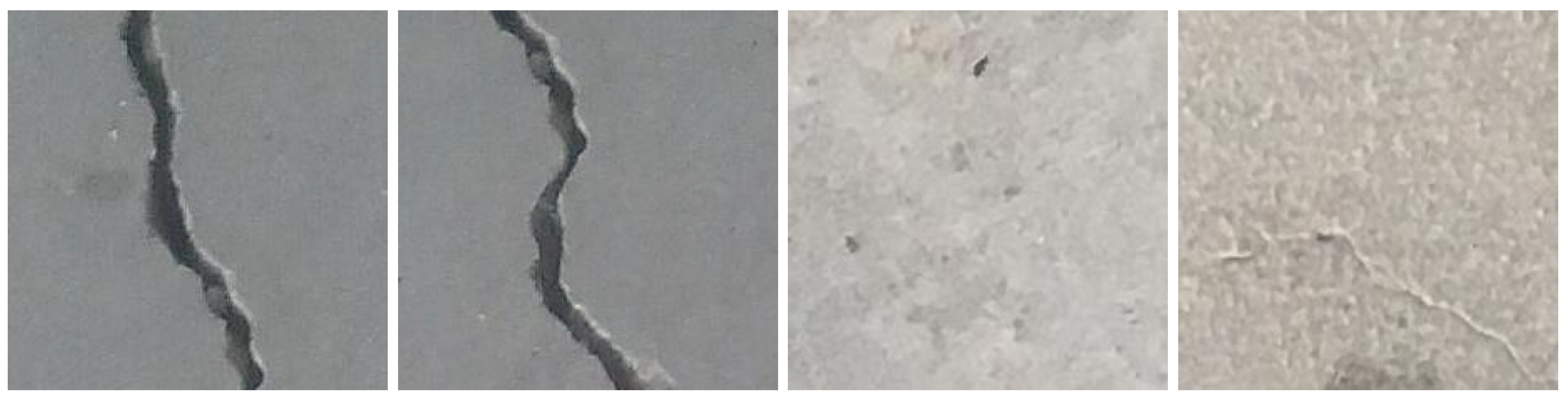
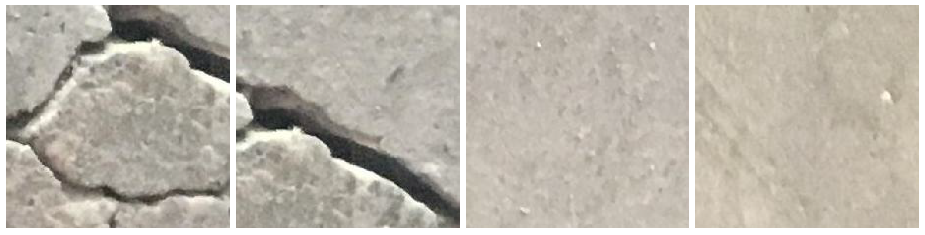
3.1. Dataset Description

The utilized dataset in this research paper is Concrete Crack Images for Classification (CCIC) [20]. It contains concrete images having cracks and non-cracks, collected from various METU Campus Buildings. The dataset is classified into positive and negative classes, referring to cracks and non-cracks images, respectively. There are 40,000 images with 227 × 227 pixels with RGB channels, and each type has 20,000 images. The dataset is generated from 458 high-resolution (4032 × 3024 pixels) images taken from floors and walls of various concrete buildings. Images are taken with the camera facing directly to the concrete surfaces keeping about a one-meter distance. The images are captured on the same day with similar illumination conditions. The concrete surface has variation because of plastering, paint, exposure, etc. But no data augmentation is applied [33]. Some cracks and non-cracks images of the used dataset are shown in Figure 2.

3.2. Dataset Splitting

Our dataset consists of 20,000 cracks and 20,000 non-cracks images, in a total of 40,000 images. We split the datasets into 2 groups, with ratios of $80\%$ and $20\%$ for the Train set as well as the Test or Validation set, respectively. After randomly splitting the dataset into train along with test sets, we obtained 31,999 images (16,000 cracks and 15,999 non-cracks images) in the train set and 8001 (4000 cracks and 4001 non-cracks) images in the test set. After using the test dataset for validation of the model, the training dataset is used for training the model and calculating various evaluation matrices. Dataset splitting is shown in

Table 1. Dataset Test-train splitting.

	Crack	Non-Crack	Total
Train	16,000	15,999	31,999
Test	4000	4001	8001
Total	20,000	20,000	40,000

briefly.

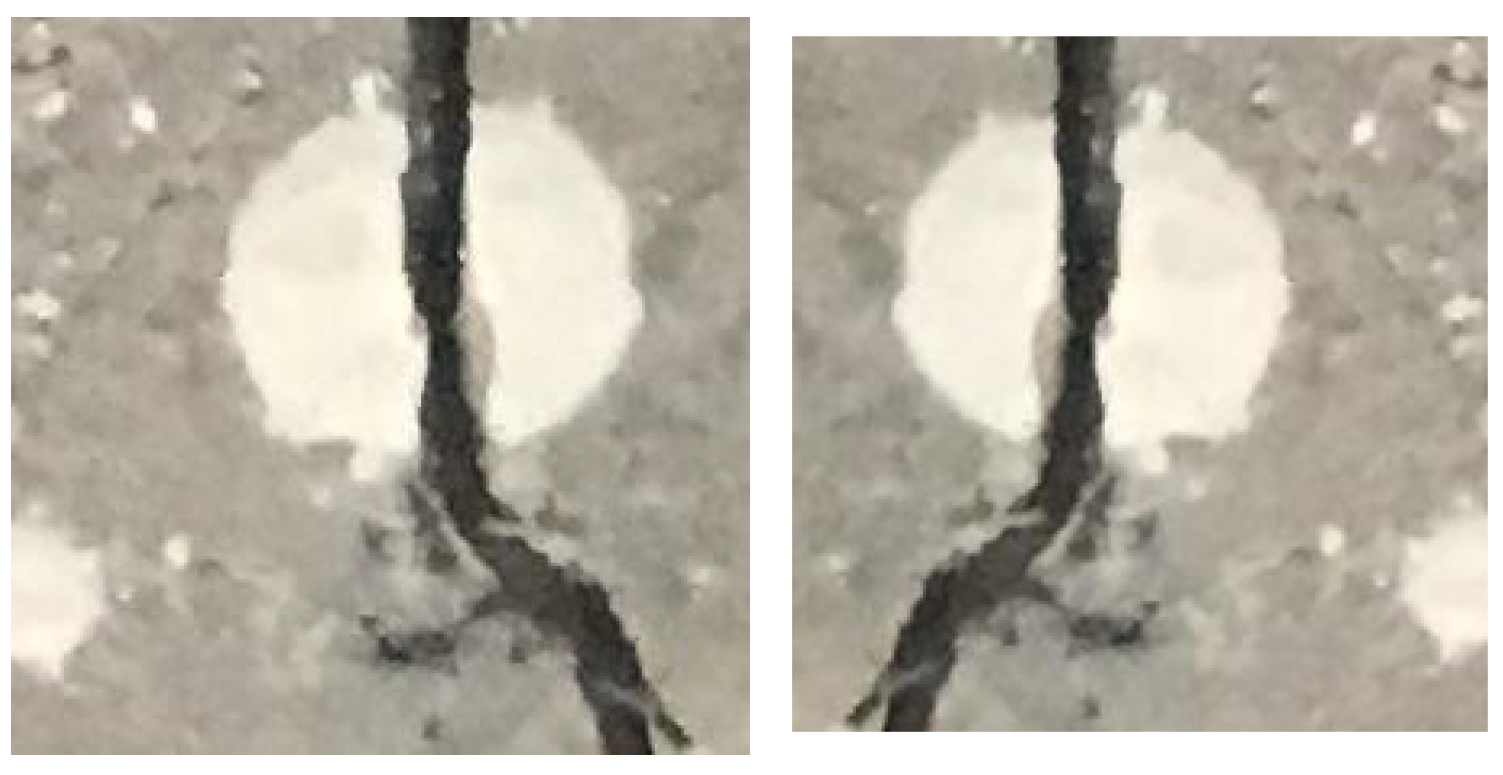
3.3. Data Augmentation and Transformation

Deep learning models perform very well on large datasets. Data augmentation is a crucial technique in deep learning for a limited dataset that enhances the size and quality of a training dataset to build a better deep learning model. There are various data augmentation techniques like flipping, cropping, rotation, color space transformation, noise injection, etc. [34]. We used data augmentation and transfer learning to overcome the lack of training data as well as get rid of overfitting. In our training dataset, we use some of the data augmentation techniques, which are described below.

3.3.1. Random-Resized-Crop Method

The random-Resized-Crop method is an augmentation method that crops a random portion of the image and resizes it according to the desired size. Such a crop is made by a random area depending on a scale and an arbitrary aspect ratio. The scale specifies a lower and upper bound for the arbitrary location of the crop, and the ratio specifies required bounds from the random aspect ratio of the yield before resizing. In our training dataset, scale = (0.8, 1.0), ratio = (0.75, 1.33) and size = (227, 227) are used. Figure 3 shows an example of this technique.

3.3.2. Random-Rotation Method

This augmentation method rotates the image by randomly selected angles from a specific range of degrees. In our training dataset, angles are selected between −15 degrees and +15 degrees. The area outside the rotated image is filled with pixel value 0. Figure 4 shows an example of the Random Rotation technique.

3.3.3. Color-Jitter Method

This augmentation method randomly changes the brightness, contrast, saturation, and hue of an image. An example of this method is shown in Figure 5.

3.3.4. Random-Horizontal-Flip Method

This augmentation method horizontally flips the given image randomly with a specified probability. Our training dataset has been flipped with $50\%$ probability. An example of a Random Horizontal Flip is exhibited in Figure 6.

We used the above data augmentation techniques for training datasets and did not use data augmentation techniques for testing test data. Besides, some preprocessing stages are applied to both train and test datasets. CCIC dataset’s image dimension is 227 × 227. But the desired input image dimension of our proposed model is 224 × 224. For this reason, preprocessing is applied to achieve desired image dimensions. Center cropping is applied on the 227 × 227 dimension image for getting a 224 × 224 dimension image. Also, we apply normalization to all images. Our pre-trained models expect input 3-channel RGB images normalized using mean of [0.485, 0.456, 0.406] and standard deviation of [0.229, 0.224, 0.225].

3.4. Design Transfer Learning Model

Image recognition has advanced remarkably, mostly because deep learning (DL) and deep convolutional neural networks (CNNs) with large-scale annotated datasets are now widely available. With enough training data, CNNs can learn data-driven, highly representative, hierarchical image characteristics. Currently, there are three main methods for effectively employing CNNs for image classification: building the CNN from scratch, using pre-trained CNN features that are available for purchase, and using unsupervised CNN pre-training with supervised fine-tuning. Transfer learning, or fine-tuning CNN models pre-trained from natural image datasets to image problems, is another efficient technique. A step in the process by which computers may examine a picture and assign it the proper label is image categorization [35,36,37].

Overall, CNN and deep learning (DL) are key components of image categorization nowadays. DL methods can tackle issues with increasingly complicated, highly variable functions. It also involves a sizable picture dataset, even one without labels. Machines can recognize and extract characteristics from images with the aid of DL. The image categorization [35,38] on CNN, therefore, generates a lot of attention. To perform tasks correctly, DL approaches need a lot of data [8]. Having access to a wealth of knowledge is not necessarily true. Pre-trained models are applied in this situation. In this study, transfer learning (TL) is the reuse of a deep learning pre-trained approach where knowledge is driven from one model to another [39].

Several well-known pre-trained models exhibit excellent performance across a range of computer vision issues. Some of them are VGG [40], ResNet [41], DenseNet [42], AlexNet [43], Inception v3 [44], GoogLeNet [45], MobileNet [46] etc. These models are trained on extensive datasets with various classes of images. Using TL methods, it is now possible to achieve very good performance on several computer vision issues with a lack of data and computing power. This paper experimented on four well-known models named VGG, ResNet, DenseNet, and AlexNet. In the following sections, we discuss these transfer learning models.

3.4.1. VGG16

VGG16 is a CNN model trained on the ImageNet dataset of over 1.2 million images from 1000 classes [40]. The architecture of the VGG16 model is depicted in Figure 7.

There are several convolutional (conv) layers, where filters with 3 × 3 kernels are used. The convolution stride and padding are fixed to 1 pixel. Max-pooling is applied, followed by some conv layers with 2 × 2 kernels, a stride of 2, and padding of 0. The input to conv layer is of fixed size 224 × 224 RGB image.

Three FC layers are added in the last part of the architecture, and the last layer is configured for 1000 classes. The Rectified Linear Unit (ReLU), a non-linear activation function is used by all hidden layers.

We apply the pre-trained VGG16 model to the proposed Transfer Learning (TL) model. We call it TL VGG16. We remove the last three FC layers and replace them with an FC2 layer such that output features match for binary classification.

3.4.2. ResNet18

ResNet is a CNN technique presented in the paper titled Deep Residual Learning for Image Recognition’ [41]. The model trained on ImageNet dataset of over 1.2 million images belonging to 1000 classes. The architecture of the ResNet18 model is depicted in Figure 8.

There are several convolutional (conv) layers. Filters with 7 × 7 kernels, strides of 2, and padding of 3 are used in the first conv layer. In the remaining conv layers, filters with 3 × 3 kernels, strides of 1, and padding of 1 are used except for some down-sampling conv with 1 × 1 kernels and stride of 2. The pattern remains the same, bypassing the input every 2 convolutions. Max-pooling is applied following the 1st conv layer with 3 × 3 kernels, a stride of 2 as well as padding of 1. The input to conv layer is of fixed size 224 × 224 RGB image.

Three FC layers are added in the last part of the architecture, and the last layer is configured for 1000 classes. Most hidden layers employ Batch Normalization, and a convolutional layer after ReLU.

We use the pre-trained ResNet18 method for the proposed TL ResNet18 model. We replace the last FC layer with a Fully-Connected FC2 layer such that output features match for binary classification.

3.4.3. DenseNet161

DenseNet161 is a CNN model proposed by Zhuang et al. [42]. They have trained their model on an ImageNet dataset of over 1.2 million images from 1000 classes. A typical architecture of the DenseNet161 model is shown in Figure 9. It can be seen that there are a series of convolution (conv) layers within it, where every layer has access to its preceding feature maps. In the first conv layer, filters with 7 × 7 kernels, strides of 2, and padding of 3 are used. Then Normalization, ReLU, and max-pooling with 3 × 3 kernels, a stride of 2, and padding of 1 are used. After the first conv layer, there are four dense blocks and each block has corresponding 6, 12, 36, and 24 dense layers. Each dense layer consists of two conv layers; the preceding conv layer has a filter with 1 × 1 kernels and stride of 1 and, the latter conv layer has a filter with 3 × 3 kernels, a stride of 1, and padding of 1. Before conv layer, Batch Normalization, and ReLU are used. In the middle of two dense-blocks transition layers with Batch Normalization, ReLU, conv layer with 1 × 1 kernels and a stride of 1 and then an AvgPool with 2 × 2 kernels, a stride of 2, and padding of 0 are used. After the 4th dense-block Batch, normalization is applied.

An FC layer is added in the last part of the architecture and configured for 1000 classes.

We used the pre-trained DenseNet161 model for the proposed TL DenseNet161 model. We have replaced the last FC layer with an FC2 layer such that output features match binary classification. The input to conv layer is of fixed size 224 × 224 RGB image.

3.4.4. AlexNet

AlexNet is a CNN model proposed by Alex Krizhevsky [43]. The model trained on ImageNet dataset of over 1.2 million images belonging to 1000 classes. The architecture of the AlexNet model is depicted in Figure 10. There are several convolutional (conv) layers. In the conv layer, filters with 11 × 11 kernels, strides of 4, and padding of 2 are used. In the 2nd conv layer, filters with 5 × 5 kernels, strides of 1, and padding of 2 are used. In the remaining three conv layers, filters with 3 × 3 kernels, strides of 1, and padding of 1 are used. Max-pooling is applied, followed by conv layers with 3 × 3 kernels, a stride of 2, and padding of 0.

Three FC layers are added in the last part of the architecture. All hidden layers use the ReLU, a non-linear activation function. Dropout with the possibility of 0.5 is utilized before the first two FC layers. The last layer is configured for 1000 classes.

We use the pre-trained AlexNet model for the proposed TL AlexNet model. We remove the last three FC layers and replace them with an FC2 layer such that output features match for binary classification. The input to conv layer is of fixed size 224 × 224 RGB image.

3.5. Experimental Setup, Model Training, and Evaluation

All the experiments take place in a Google Colaboratory notebook with a GPU runtime. Training is taken repeatedly throughout a number of epochs. We train our models for 30 epochs. After using the test dataset for validation of the model, the training dataset is applied for training the model. We use the PyTorch library primarily developed by the AI Research lab of Facebook. We implement the PyTorch data loader to take data of 128 batch size. We utilize the same hyperparameters optimization setup for all architectures.

Table 2. Hyperparameters of different TL methods.

Parameters	Parameters Value
Batch size	128
Optimizer	Adam
Learning rate	0.001
Betas	(0.9, 0.999)
Eps	1 × ${10}^{-8}$
Weight decay	0
Criterion	Cross Entropy Loss

shows the used hyperparameters in the experimental setup.

We determine the cross-entropy loss on the train as well as test sets for each epoch. We employ the Adam optimizer [47] using the mentioned parameters value.

In Figure 11, train losses, validation losses along with train accuracies as well as validation accuracies of each TL method are depicted. In the experimental observation, we see that there is no over-fitting occurring in any of the TL models. In the first row of Figure 11, the TL VGG16 models show that both train and validation loss is reduced very quickly, and they do not improve for a higher number of epochs. The TL ResNet18 model’s train and validation loss are decreased gradually and the validation loss is always lower than the training loss with very little difference. The TL DenseNet161 model’s train and validation loss follow an almost similar pattern to the TL ResNet18 model. On the other hand, we see in the training and validation loss of TL AlexNet that the bare difference between the two lines, unlike ResNet18 and DenseNet161. Hence, we can conclude this model converge quickly with very good generalization capability. Whereas, train along with validation accuracy of several TL methods are presented in the second row Figure 11. We see a similar pattern like the train and validation loss of different TL models. The ResNet18 and DenseNet161 follow the same pattern: validation accuracy is always greater than the training accuracy. Also, train accuracy is always less than the validation accuracy in the VGG16 model. But the TL AlexNet model shows the different patterns, the train, and validation accuracy overlap, and achieves high accuracy among other models. The AlexNet shows good generalization among others.

We clearly see that AlexNet achieves the best score for the lowest training and validation losses among all other models. Also, we clearly see that AlexNet achieves the best score for the highest training and validation accuracies among all other models.

4. Result Exploration and Argument

Through the confusion matrix, we can find out the P, R, F1, and Accuracy. These are the criteria for evaluating the classification model. Confusion matrix has four keywords of this including True Positive, False Positive, False Negative, and True Negative [48].

We can define Precision, Recall, F1-score, and Accuracy mathematically by using the Equations (1)–(4) respectively.

$$Precision,P=\frac{TP}{TP+FP}$$

(1)

$$Recall,R=\frac{TP}{TP+FN}$$

(2)

$$F1-score,F1=2\times \frac{P\times R}{P+R}$$

(3)

$$Accuracy=\frac{Numberofcorrectpredictions}{Totalnumberofpredictionsmade}$$

(4)

After 30 epochs of training of all TL models, an evaluation is made on a test dataset consisting of 8001 images where 4000 images are cracks and 4001 images are non-cracks. Figure 12 illustrates the confusion matrix of all models.

The TL VGG16 predicts 3996 (TP) cracks and 3990 (TN) non-cracks images correctly, as well as 4 (FN) cracks images predicted as non-crack, and 11 (FP) non-cracks images predicted as cracks Figure 12a. The number of FN is minimum among other models.

The TL ResNet18, on the other hand, predicts 3988 (TP) cracks and 3959 (TN) non-cracks images correctly, as well as 12 (FN) cracks images predicted as non-crack and 42 (FP) non-cracks images predicted as cracks Figure 12b. In this case, the number of FP is the highest among other models.

We can see in the TL DenseNet161 model’s confusion matrix Figure 12c, that it predicts 3994 (TP) cracks and 3981 (TN) non-cracks images correctly, as well as 8 (FN) cracks images predicted as non-crack and 20 (FP) non-cracks image predicted as cracks. TL AlexNet Figure 12d shows the balance between FN and FP and shows the minimum number of FP (3 FP) among all other models.

Table 3. Various scores were calculated in the test dataset (CCIC) for different TL models after 30 epochs of training where P = Precision, R = Recall, F1 = F1-score, Sup = Support, A = Accuracy, CK = Cohen’s Kappa.

Model		P (%)	R (%)	F1 (%)	Sup	A (%)	MCC (%)	CK (%)
TL VGG16	Crack	99.73	99.90	99.81	4000	99.81	99.6252	99.6250
	Non-crack	99.90	99.73	99.81	4001
TL ResNet18	Crack	98.96	99.70	99.33	4000	99.33	98.6529	98.6502
	Non-crack	99.70	98.95	99.32	4001
TLDenseNet161	Crack	99.50	99.85	99.68	4000	99.68	99.3507	99.3501
	Non-crack	99.85	99.50	99.67	4001
TL AlexNet	Crack	99.92	99.80	99.86	4000	99.86	99.7251	99.7250
	Non-crack	99.80	99.93	99.86	4001

displays several standard assessment scores, with the number of samples utilized during the evaluation represented in the Support column which is denoted as Sup.

From Table 3, we can conclude that TL AlexNet achieves the highest $99.86\%$ F1 scores and $99.86\%$ accuracies among other models and precision of $99.92\%$ on cracks and recall of $99.93\%$ on non-cracks. In the case of popular statistical tests named MCC and CK (Cohen’s Kappa), AlexNet performs better than others. The values of MCC and CK are almost the same, we took 4 digits after the decimal point. Although, AlexNet achieves the best validation accuracy of $99.90\%$ during the 13th epoch training, shown in

Table 4. Performance measurement of used TL methods during 30 epochs of training where MA_E = Maximum Accuracy at epoch, MinA_E = Minimum Accuracy at epoch, Avg_acc = Average Accuracy.

Model	Train/Test	Max Acc (%)	MA_E	Min Acc (%)	MinA_E	Avg_acc (%)
TL VGG16	Train	99.76	30	98.06	1	99.61
	Test	99.86	29	99.65	17	99.78
TL ResNet18	Train	99.09	29	95.31	1	98.74
	Test	99.41	18	98.09	1	99.22
TL DenseNet161	Train	99.51	25	96.68	1	99.24
	Test	99.68	27	99.29	1	99.60
TL AlexNet	Train	99.85	24	98.34	1	99.72
	Test	99.90	13	99.58	20	99.84
All	Train Max Acc	99.85	TL AlexNet at Epoch 24
	Test Max Acc	99.90	TL AlexNet at Epoch 13
	Both Max Acc	99.90	TL AlexNet at Epoch 13

.

As a succinct outline of every TL algorithm throughout training as well as validation, Table 4 displays the highest, lowest, and average accuracy. From the summary, we can conclude that AlexNet models achieve the best train accuracy of $99.85\%$ on the 24th epoch and the best validation accuracy of $99.90\%$ on the 13th epoch among all other models.

Table 5. Training time per-epoch of TL models.

Model	Duration Per-Epoch (h:mm:ss)	Remarks
TL VGG16	0:08:46.729322	3rd place
TL ResNet18	0:03:35.636223	2nd place
TL DenseNet161	0:13:39.103467	Lowest place
TL AlexNet	0:02:53.093954	1st place
TL AlexNet takes the 1st position by achieving the least training time

shows the training duration of each epoch during training on Google Colaboratory GPU runtime. The TL AlexNet achieves 1st place by taking minimum training time among the other models.

We also depicted the receiver operating characteristic (ROC) curve for comparing the models in the case of appropriate classification results. It is measured based on the performance of the false positive rate and true positive rate respectively. Figure 13 shows the ROC curve of different TL models in our works. In this figure, we denote four curves of red, green, blue, and orange colored for AlexNet, DenseNet, VGG16, and ResNet18 models. All models’ performances are good. On the left side of this figure, all curves are looking together. For understanding better, we observed it as zoom out which is shown in the right portion of the figure. From this figure, we can see that AlexNet places the highest position over other models.

We also presented another way of evaluating the performance of models named the precision-recall (PR) curve. Figure 14 shows the PR curve of different TL models in our works. In this figure, we mark four curves of red, green, blue, and orange colored for AlexNet, DenseNet, VGG16, and ResNet18 models. In the upper side of this figure, all curves are looking together. For understanding better, we observed it as zoom out which is shown in the down portion of the figure. From this figure, we can see that all models’ performance is good.

In addition, we used the external dataset Building Wall Crack Images (BWCI) from Kaggle to validate our models. This is an open-source dataset. BWCI consists of wall crack images with 27 × 27 pixels.

Table 6. Summary of external dataset (BWCI).

Image Folder	No. of Crack Images	No. of Noncrack Images	Total
Test	500	500	1000
Train	1250	1250	2500
Validation	500	500	1000

shows the description of the dataset and a few samples are shown in Figure 15.

Table 7. Performance result of external dataset (BWCI) where P = Precision, R = Recall, F1 = F1-score, A = Accuracy.

Model		P (%)	R(%)	F1 (%)	A (%)	MCC (%)	CK (%)
TL VGG16	Crack	99.80	1.00	99.90	99.90	99.8000	99.7998
	Non-crack	1.00	99.80	99.90
TL ResNet18	Crack	99.40	99.80	99.60	99.60	99.1999	99.1992
	Non-crack	99.80	99.40	99.60
TLDenseNet161	Crack	99.60	1.00	99.80	99.80	99.6004	99.5996
	Non-crack	1.00	99.60	99.80
TL AlexNet	Crack	1.00	99.80	99.90	99.90	99.7999	99.7997
	Non-crack	99.80	1.00	99.90

represents the result of all models on the external dataset. We used only the test folder dataset to validate the models. It can be seen that the performance for both CCIC and external datasets BWCI are almost same.

Two statistical tests have been carried out, named the Matthews correlation coefficient (MCC) and Cohen’s Kappa Statistic [49] for comparing the performance. Matthews correlation coefficient (MCC) is a popular performance metric that is used in the case of an imbalanced dataset. Although the utilized dataset in this paper is a balanced dataset, it is defined by the following mathematical equation number 5.

$$MCC=\frac{TP\times TN-FP\times FN}{\sqrt{(TP+FP)\times (TP+FN)\times (TN+FP)\times (TN+FN)}}$$

(5)

The range of MCC is [−1–1]. The value of MCC is near to 1 is better. All of the utilized models perform well. Their values are near to 1. That means, the models classified the crack images accurately.

Cohen’s Kappa Statistic is applied to assess the degree of agreement between two raters who categorize objects into mutually exclusive groups which are shown mathematically in Equation (6).

$$CK=\frac{(p_o-p_e)}{(1-p_e)}$$

(6)

Here, $p_o$ is the relative agreement of raters’ observation. $p_e$ denotes the theoretical probability of random agreement. we can calculate $p_o$ and $p_e$ between the raters by using the Equations (7)–(10).

$$p_o=\frac{TP+TN}{TP+TN+FP+FN}$$

(7)

$$p_e=probabilityofPositive+probabilityofNegative$$

(8)

Here,

$$ProbabilityofPositive=\frac{TP+FP}{TP+TN+FP+FN}\times \frac{TP+FN}{TP+TN+FP+FN}$$

(9)

and

$$ProbabilityofNegative=\frac{FP+TN}{TP+TN+FP+FN}\times \frac{FN+TN}{TP+TN+FP+FN}$$

(10)

Cohen’s Kappa is always between 0 and 1, with 0 indicating no agreement as well as 1 showing full agreement between the 2 raters. All models CK is almost full agreement between the actual and predictors. Table 3, shows the performance of the CCIC dataset, and Table 7 shows the performance metrics of the external dataset.

5. Discussion

Noticeable research has been done for detecting concrete surface cracks and researchers concluded different solutions. In this segment, we discuss and liken our presented model to the existing similar study.

Table 8. Summary of publications using CNN-based transfer learning techniques for cracks detection.

SN	Reference	Base Model or Method	Accuracy	Dataset
01	[14]	VGG16	90%	Beam, column, wall and joint brace images of a building
02	[16]	FF-BLS	96.72%	CCIC dataset
03	[17]	VGG16	94%, 98%	Fatigue cracks in gusset plate joints in steel bridges
04	[12]	SegNet	99%	Concrete pavement, asphalt pavement, and bridge deck cracks images
05	[18]	VGG16	92.27%	Concrete surfaces dataset collected from the Danish Technological Institute
06	[21]	DCNN model	97.70%	CCIC dataset
07	[23]	ResNet18	98.80%	Roads and bridges crack images
08	[24]	GoogLeNet Inception V3	97.30%	Wall images at college of environmental resources of Fuzhou University
09	[13]	MobileNet	99.59%	Wall, pavements, bridge deck images
10	[26]	YOLOv5	88.10%	Asphalt crack pavement images
11	Proposed	AlexNet	99.90%	CCIC dataset

shows the summary of several publications for cracks detection using CNN. SegNet and MobileNet achieve $99\%$ and $99.59\%$ accuracy, respectively. Other mentioned papers achieve less than $99\%$ accuracy except for our proposed TL AlexNet model, which obtains 1st position by achieving an accuracy of $99.90\%$. That is why our proposed transfer learning (TL) approach to the AlexNet model is an excellent candidate for concrete surface cracks detection.

6. Conclusions

In this paper, we applied a deep convolutional neural network based on transfer learning models to detect crack images using a popular crack dataset named Concrete Crack Images for Classification (CCIC). We utilized four transfer learning models for the experimental setup containing VGG16, ResNet18, DenseNet161, and AlexNet. As a performance metric, we used four terms named accuracy, recall, precision, and f1-score. Among the utilized models, AlexNet outperforms all the cases of performance metrics by achieving the accuracy of $99.90\%$, P of $99.92\%$, R of $99.80\%$, and F1-score of $99.86\%$. We also showed the training duration per epoch of all models. In this case, AlexNet achieves the first position in less time. In future work, we will conduct further research to provide a robust description of changing knowledge in our model.

References

1. Aggelis, D.G.; Alver, N.; Chai, H.K. Health Monitoring of Civil Infrastructure and Materials. Sci. World J. 2014, 2014, 435238. [Google Scholar] [CrossRef] [PubMed]
2. Gavilán, M.; Balcones, D.; Marcos, O.; Llorca, D.F.; Sotelo, M.A.; Parra, I.; Ocaña, M.; Aliseda, P.; Yarza, P.; Amírola, A. Adaptive road crack detection system by pavement classification. Sensors 2011, 11, 9628–9657. [Google Scholar] [CrossRef] [PubMed]
3. Wang, P.; Hu, Y.; Dai, Y.; Tian, M. Asphalt pavement pothole detection and segmentation based on wavelet energy field. Math. Probl. Eng. 2017, 2017, 1604130. [Google Scholar] [CrossRef]
4. Yamaguchi, T.; Nakamura, S.; Saegusa, R.; Hashimoto, S. Image-based crack detection for real concrete surfaces. IEEJ Trans. Electr. Electron. Eng. 2008, 31, 128–135. [Google Scholar] [CrossRef]
5. Tsai, Y.C.; Kaul, V.; Mersereau, R.M. Critical assessment of pavement distress segmentation methods. J. Transp. Eng. 2010, 136, 11–19. [Google Scholar] [CrossRef]
6. Albert, P.; Nii, A. Evaluating pavement cracks with bidimensional empirical mode decomposition. EURASIP J. Adv. Signal Process. 2008, 2008, 861701. [Google Scholar] [CrossRef]
7. Peggy, S.; Jean, D.; Vincent, L.; Dominique, B. Automation of pavement surface crack detection using the continuous wavelet transform. In Proceedings of the 2006 International Conference on Image Processing, Atlanta, GA, USA, 8 October 2006. [Google Scholar]
8. Yann, L.; Yoshua, B.; Geoffrey, H. Deep learning. Nature 2015, 521, 436–444. [Google Scholar] [CrossRef]
9. Valuevaa, M.; Nagornovb, N.; Lyakhovab, P.; Valueva, G.; Chervyakova, N. Application of the residue number system to reduce hardware costs of the convolutional neural network implementation. Math. Comput. Simul. 2020, 177, 232–243. [Google Scholar] [CrossRef]
10. Hasan, K.F.; Overall, A.; Ansari, K.; Ramachandran, G.; Jurdak, R. Security, privacy and trust: Cognitive internet of vehicles. arXiv 2021, arXiv:2104.12878. [Google Scholar]
11. Jinsong, Z.; Song, J. An intelligent classification model for surface defects on cement concrete bridges. Appl. Sci. 2020, 10, 972. [Google Scholar] [CrossRef]
12. Chen, T.; Cai, Z.; Zhao, X.; Chen, C.; Liang, X.; Zou, T.; Wang, P. Pavement crack detection and recognition using the architecture of segNet. J. Ind. Inf. Integr. 2020, 18, 100144. [Google Scholar] [CrossRef]
13. Sayyed, B.A.; Reshul, W.; Sameer, K.; Anurag, S.; Santosh, K. Wall Crack Detection Using Transfer Learning-based CNN Models. In Proceedings of the 2020 IEEE 17th India Council International Conference (INDICON), New Delhi, India, 10–13 December 2020. [Google Scholar]
14. Yuqing, G.; Khalid, M.M. Deep transfer learning for image-based structural damage recognition. Comput. Civ. Infrastruct. Eng. 2018, 33, 748–768. [Google Scholar] [CrossRef]
15. Zheng, Z.; Qi, H.; Zhuang, L.; Zhang, Z. Automated rail surface crack analytics using deep data-driven models and transfer learning. Sustain. Cities Soc. 2021, 70, 102898. [Google Scholar] [CrossRef]
16. Zhang, Y.; Yuen, K.V. Crack detection using fusion features-based broad learning system and image processing. Comput. Civ. Infrastruct. Eng. 2021, 36, 1568–1584. [Google Scholar] [CrossRef]
17. Cao, V.D.; Hidehiko, S.; Suichi, H.; Takayuki, O.; Chitoshi, M. A vision-based method for crack detection in gusset plate welded joints of steel bridges using deep convolutional neural networks. Autom. Constr. 2019, 102, 217–229. [Google Scholar] [CrossRef]
18. Wilson, R.L.S.; Diogo, S.L. Concrete cracks detection based on deep learning image classification. Multidiscip. Digit. Publ. Inst. Proc. 2018, 2, 489. [Google Scholar] [CrossRef]
19. Xiuying, M. Concrete Crack Detection Algorithm Based on Deep Residual Neural Networks. Sci. Program. 2021, 2021, 3137083. [Google Scholar] [CrossRef]
20. Ozgenel, Ç.F.; Sorguç, G.A. Performance comparison of pretrained convolutional neural networks on crack detection in buildings. In Proceedings of the 35th International Symposium on Automation and Robotics in Construction (ISARC 2018), Berlin, Germany, 20–25 July 2018. [Google Scholar]
21. Tien-Thinh, L.; Van-Hai, N.; Minh Vuong, L.E. Development of deep learning model for the recognition of cracks on concrete surfaces. Appl. Comput. Intell. Soft Comput. 2021, 2021, 18858545. [Google Scholar] [CrossRef]
22. Ren, Y.; Huang, J.; Hong, Z.; Lu, W.; Yin, J.; Zou, L.; Shen, X. Image-based concrete crack detection in tunnels using deep fully convolutional networks. Constr. Build. Mater. 2020, 234, 117367. [Google Scholar] [CrossRef]
23. Yang, C.; Chen, J.; Li, Z.; Huang, Y. Structural Crack Detection and Recognition Based on Deep Learning. Appl. Sci. 2021, 11, 2868. [Google Scholar] [CrossRef]
24. Wu, L.; Lin, X.; Chen, Z.; Lin, P.; Cheng, S. Surface crack detection based on image stitching and transfer learning with pretrained convolutional neural network. Struct. Control Health Monit. 2021, 28, e2766. [Google Scholar] [CrossRef]
25. Kong, X.; Li, J. Vision-based fatigue crack detection of steel structures using video feature tracking. Comput. Civ. Infrastruct. Eng. 2018, 33, 783–799. [Google Scholar] [CrossRef]
26. Guo, X.H.; Bao, L.H.; Zhong, Y.L.; Li, H.; Ping, L. Pavement Crack Detection Method Based on Deep Learning Models. Wirel. Commun. Mob. Comput. 2021, 2021, 5573590. [Google Scholar] [CrossRef]
27. Li, W.; Chen, H.; Zhang, Y.; Shi, Y. Track slab crack detection based on full convolutional neural network. In Proceedings of the 2021 4th International Conference on Advanced Algorithms and Control Engineering (ICAACE 2021), Sanya, China, 29–31 January 2021. [Google Scholar]
28. Gerivan, S.J.; Janderson, F.; Cristian, M.; Ramiro, D.; Alberto, C.J.; Bruno, J.T.F. Ceramic cracks segmentation with deep learning. Appl. Sci. 2021, 11, 6017. [Google Scholar] [CrossRef]
29. Wei, Y.; Wei, Z.; Xue, K.; Yao, W.; Wang, C.; Hong, Y. Automated detection and segmentation of concrete air voids using zero-angle light source and deep learning. Autom. Constr. 2021, 130, 103877. [Google Scholar] [CrossRef]
30. Diana, A.A.; Anand, N.; Eva, L.; Prince, A.G. Deep Learning based Thermal Crack Detection on Structural Concrete Exposed to Elevated Temperature. Adv. Struct. Eng. 2021, 24, 1896–1909. [Google Scholar] [CrossRef]
31. Zhang, J.; Lu, C.; Wang, J.; Wang, L.; Yue, X.G. Concrete cracks detection based on FCN with dilated convolution. Appl. Sci. 2019, 9, 2686. [Google Scholar] [CrossRef]
32. Liu, Z.; Cao, Y.; Wang, Y.; Wang, W. Computer vision-based concrete crack detection using U-net fully convolutional networks. Autom. Constr. 2019, 104, 129–139. [Google Scholar] [CrossRef]
33. Lei, Z.; Fan, Y.; Yimin, D.Z.; Ying, J.Z. Road crack detection using deep convolutional neural network. In Proceedings of the 2016 IEEE International Conference on Image Processing (ICIP), Phoenix, AZ, USA, 25–28 September 2016. [Google Scholar]
34. Connor, S.; Taghi, M.K. A survey on image data augmentation for deep learning. J. Big Data 2019, 6, 60. [Google Scholar] [CrossRef]
35. Shin, H.C.; Roth, H.R.; Gao, M.; Lu, L.; Xu, Z.; Nogues, I.; Yao, J.; Mollura, D.; Summers, R.M. Deep convolutional neural networks for computer-aided detection: CNN architectures, dataset characteristics and transfer learning. IEEE Trans. Med. Imaging 2016, 35, 1285–1298. [Google Scholar] [CrossRef]
36. Talukder, M.A.; Islam, M.M.; Uddin, M.A.; Akhter, A.; Hasan, K.F.; Moni, M.A. Machine learning-based lung and colon cancer detection using deep feature extraction and ensemble learning. Expert Syst. Appl. 2022, 205, 117695. [Google Scholar] [CrossRef]
37. Bala, M.; Ali, M.H.; Satu, M.S.; Hasan, K.F.; Moni, M.A. Efficient Machine Learning Models for Early Stage Detection of Autism Spectrum Disorder. Algorithms 2022, 15, 166. [Google Scholar] [CrossRef]
38. Bengio, Y.; Lecun, Y.; Hinton, G. Deep learning for AI. Commun. ACM 2021, 64, 58–65. [Google Scholar] [CrossRef]
39. Kim, D.; MacKinnon, T. Artificial intelligence in fracture detection: Transfer learning from deep convolutional neural networks. Clin. Radiol. 2018, 73, 439–445. [Google Scholar] [CrossRef]
40. Karen, S.; Andrew, Z. Very deep convolutional networks for large-scale image recognition. arXiv 2015, arXiv:1409.1556. [Google Scholar]
41. He, K.; Zhang, X.; Ren, S.; Sun, J. Deep residual learning for image recognition. In Proceedings of the IEEE Conference on Computer Vision and Pattern Recognition (CVPR), Las Vegas, NV, USA, 27–30 June 2016. [Google Scholar]
42. Huang, G.; Liu, Z.; Van Der Maaten, L.; Weinberger, K.Q. Densely connected convolutional networks. In Proceedings of the IEEE Conference on Computer Vision and Pattern Recognition, Honolulu, HI, USA, 21–26 July 2017. [Google Scholar]
43. Alex, K. One weird trick for parallelizing convolutional neural networks. arXiv 2014, arXiv:1404.5997. [Google Scholar]
44. Christian, S.; Vincent, V.; Sergey, L.; Jon, S.; Zbigniew, W. Rethinking the inception architecture for computer vision. In Proceedings of the IEEE Conference on Computer Vision and Pattern Recognition(CVPR), Las Vegas, NV, USA, 27–30 June 2016. [Google Scholar]
45. Szegedy, C.; Liu, W.; Jia, Y.; Sermanet, P.; Reed, S.; Anguelov, D.; Erhan, D.; Vanhoucke, V.; Rabinovich, A. Going Deeper with Convolutions. In Proceedings of the IEEE Conference on Computer Vision and Pattern Recognition (CVPR), Boston, MA, USA, 7–12 June 2015. [Google Scholar]
46. Sandler, M.; Howard, A.; Zhu, M.; Zhmoginov, A.; Chen, L.C. Mobilenetv2: Inverted residuals and linear bottlenecks. In Proceedings of the IEEE Conference on Computer Vision and Pattern Recognition (CVPR), Salt Lake City, UT, USA, 18–22 June 2018. [Google Scholar]
47. Alex, K. Adam: A method for stochastic optimization. arXiv 2014, arXiv:1412.6980. [Google Scholar]
48. Hossain, M.B.; Iqbal, S.H.S.; Islam, M.M.; Akhtar, M.N.; Sarker, I.H. Transfer learning with fine-tuned deep CNN ResNet50 model for classifying COVID-19 from chest X-ray images. Inform. Med. Unlocked 2022, 30, 100916. [Google Scholar] [CrossRef]
49. Chicco, D.; Jurman, G. The advantages of the Matthews correlation coefficient (MCC) over F1 score and accuracy in binary classification evaluation. BMC Genom. 2020, 21, 6. [Google Scholar] [CrossRef]
Figure 1. A block diagram of the proposed methodology.
Algorithms 15 00287 g001
Figure 2. Sample crack and non-crack images of the CCIC dataset.
Algorithms 15 00287 g002
Figure 3. Example of Random Resized Crop transformation. (Left is the original image).
Algorithms 15 00287 g003
Figure 4. Example of Random Rotation transformation. (Left is the original image).
Algorithms 15 00287 g004
Figure 5. Example of Color Jitter transformation. (Left is the original image).
Algorithms 15 00287 g005
Figure 6. Example of Random Horizontal Flip transformation. (Left is the original image).
Algorithms 15 00287 g006
Figure 7. VGG16 and TL VGG16 architectures.
Algorithms 15 00287 g007
Figure 8. ResNet18 and TL ResNet18 architecture.
Algorithms 15 00287 g008
Figure 9. DenseNet161 and TL DenseNet161 architectures.
Algorithms 15 00287 g009
Figure 10. AlexNet and TL AlexNet architecture.
Algorithms 15 00287 g010
Figure 11. Loss and accuracy of all TL models both in Train and validation.
Algorithms 15 00287 g011
Figure 12. Confusion matrix of TL VGG16, TL ResNet18, TL DenseNet161, and TL AlexNet.
Algorithms 15 00287 g012
Figure 13. ROC curve of different TL models.
Algorithms 15 00287 g013
Figure 14. PR curve of different TL models.
Algorithms 15 00287 g014
Figure 15. Sample crack and non-crack images of external dataset.
Algorithms 15 00287 g015