
Root Cause Tracing Using Equipment Process Accuracy Evaluation for Looper in Hot Rolling
1
National Engineering Research Center for Advanced Rolling Technology and Intelligent Manufacturing, University of Science and Technology Beijing, Beijing 100083, China
2
School of Automation and Electrical Engineering, University of Science and Technology Beijing, Beijing 100083, China
*
Author to whom correspondence should be addressed.
Algorithms 2024, 17(3), 102; https://doi.org/10.3390/a17030102
Submission received: 22 January 2024
/
Revised: 17 February 2024
/
Accepted: 20 February 2024
/
Published: 26 February 2024
(This article belongs to the Special Issue Data-Driven Intelligent Modeling and Optimization Algorithms for Industrial Processes)
Abstract
:The concept of production stability in hot strip rolling encapsulates the ability of a production line to consistently maintain its output levels and uphold the quality of its products, thus embodying the steady and uninterrupted nature of the production yield. This scholarly paper focuses on the paramount looper equipment in the finishing rolling area, utilizing it as a case study to investigate approaches for identifying the origins of instabilities, specifically when faced with inadequate looper performance. Initially, the paper establishes the equipment process accuracy evaluation (EPAE) model for the looper, grounded in the precision of the looper’s operational process, to accurately depict the looper’s functioning state. Subsequently, it delves into the interplay between the EPAE metrics and overall production stability, advocating for the use of EPAE scores as direct indicators of production stability. The study further introduces a novel algorithm designed to trace the root causes of issues, categorizing them into material, equipment, and control factors, thereby facilitating on-site fault rectification. Finally, the practicality and effectiveness of this methodology are substantiated through its application on the 2250 hot rolling equipment production line. This paper provides a new approach for fault tracing in the hot rolling process.
1. Introduction
In the contemporary industrial, agricultural, and construction sectors, hot-rolled strip products have become increasingly vital, leading to their production volume representing a significant portion of total steel output for steel companies. This has positioned the hot-rolled production line as a foundational element for these companies [1]. Advancements in traditional production methods, combined with the progression of computer technology, have markedly increased automation within the hot continuous rolling process [2], enhancing both the volume and quality of rolling output. Nevertheless, there has been a growing demand for higher quality in hot-rolled strip products in recent years. This surge in demand imposes more rigorous requirements on the hot-rolling production process and the precision of the equipment used. The challenge of improving the quality of plates and strips while simultaneously reducing the scrap rate represents a crucial developmental direction for steel companies and the plate and strip production industry [3].
As shown in Figure 1, the hot rolling process is inherently complex, exhibiting dynamic and nonlinear attributes. It involves numerous control loops and thousands of process variables that critically influence product quality, epitomizing a sophisticated industrial process [4]. When issues arise in any part of the process or equipment, it can significantly impact the entire production line, ultimately affecting the company’s profitability. Therefore, promptly identifying and analyzing these problematic links or equipment is essential.
Modern hot tandem rolling technology is characterized by its complexity, particularly in controlling temperature and rolling force [5], which can lead to fluctuations in product quality. To improve the stability of hot continuous rolling production, typical strategies involve focusing on critical stability-affecting factors and exploring enhancements for processes and equipment performance. Various research methodologies have been employed to address these challenges. For instance, a data-driven dynamic concurrent kernel canonical correlation analysis (DCKCCA) method was utilized for diagnosing CAP-thickness-related faults [6]. Additionally, ref. [7] developed a fault diagnosis method using two-dimensional time–frequency images and data enhancement, training a convolutional neural network (CNN)-based model for this purpose. A combination of continuous wavelet transform and a deep convolutional generative adversarial network (DCGAN) was proposed for tackling uneven data distribution in rolling bearing fault diagnosis [8]. Modified independent component analysis (MICA) was used to construct a multivariate statistical process monitoring model for detecting and analyzing chatter in hot strip mill processes [9]. Furthermore, a data-driven key performance indicator (KPI) prediction and diagnosis scheme was developed [10], offering a simplified alternative to the standard partial least squares (PLS) method.
However, most existing methods primarily focus on surface data characteristics, inferring the superficial causes of faults based on data traits. Consequently, while these methods can locate the faulty link or equipment, they often fail to identify the underlying root cause. This paper seeks to address this limitation by analyzing the problem from the perspectives of production continuity, product quality stability, and extreme specification production capacity. By examining the issue from exterior to interior layers, this study aims to identify the fundamental cause of faults. Specifically, the finishing rolling area of the hot tandem rolling production line is used as a case study, categorizing production stability factors into material, equipment, and control aspects in Table 1.
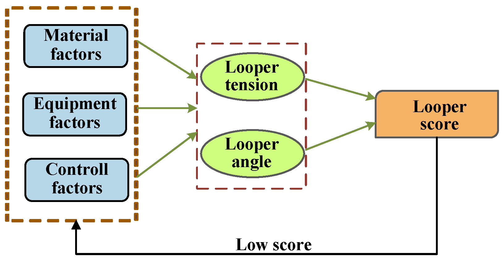
There is much related equipment involved in the finishing rolling area, and the looper can ensure the stability of the strip during the rolling process, control the shape and size of the strip, and reduce surface defects of the strip, etc. [11]; so, here we take the looper as a case study to trace its root cause. When identifying a low EPAE score for the looper during production, as Figure 2 shows, instead of examining surface-level faults and errors such as looper angle and looper tension, the focus shifts towards investigating the more profound issues depicted in the figure below. Based on the EPAE model, this paper designs a root-cause-traceability algorithm to analyze material factors, equipment factors, and control factors, to ensure that the root cause of the problem can be quickly located after an abnormality occurs.
This paper considers the problem of root cause traceability in looper equipment under the framework of production stability in the hot rolling area, inspired by the [12,13,14]. First, this paper elucidates the physical structure and operational principles of the looper. Subsequently, it delineates the precision indices for controlling the looper in each operational process and establishes the EPAE model for the looper. Then, an analysis is conducted to explore the relationship between the EPAE model of the looper and production stability. Based on this, a root-cause-traceability algorithm is proposed. In addition, actual data pertaining to loopers within the 2250 hot rolling equipment production line were used to trace the root cause, identifying the primary factors most likely contributing to a low looper score. The main contributions of the paper can be summarized as the following points.
- This paper initiates its approach from the foundational layer of production stability and analyzes problems that may arise in the production process, which is different from most existing work on fault diagnosis.
- An EPAE model based on the actual working process of the looper is proposed. This model aims to improve the interpretability of subsequent causal relationship modeling.
- A root-cause-tracing algorithm is proposed and its viability is assessed by using available actual production data.
The root-cause-tracing algorithm is a brand-new diagnostic algorithm proposed by this paper for industrial processes. It consists of data processing, building neural networks, and calculating weights. Different from previous fault diagnosis algorithms, this algorithm is committed to finding deeper problems, rather than just locating the device where the fault occurred. The calculation of weights is the highlight of this algorithm, this part converts the problem of fault location into a problem of solving a system of equations, and converts the possibility of fault occurrence into the weight of each eigenvalue. And when constructing the system of equations, both new data and past data are used to construct the system of equations. With past data as a reference, the solution is more reliable.
The remainder of the paper is structured as follows: Section 2 starts from the control accuracy of the looper and then constructs the EPAE model of the looper; Section 3 analyzes the relationship between the EPAE score and production stability and proposes a root-cause-traceability algorithm; Section 4 uses existing data to verify the root-cause-tracing algorithm and analyze its feasibility; Section 5 summarizes the findings of this paper and suggests some potential future directions.
2. EPAE Model of Looper
2.1. Physical Structure of the Looper
In the rolling process of hot-rolled plate and strip, the looper plays an important role. It stabilizes the tension between the stands, adjusts the flow rate between the stands, and ensures a constant set amount. Precisely controlling the tension and sleeve volume of the finishing rolling loop contributes to enhanced production stability, reduces the risk of accidents, and reduces the shear loss caused by the reduction in strip width [15]. Especially when rolling thin strips, precise control of the looper is crucial. Figure 3 illustrates its structure.
The end of the looper rod is connected to the looper arm on the transmission side, keeping a certain distance from the hinge point [16]. The looper shaft is installed on the exit side of the previous stand, below the rolling line. When the looper moves to the highest position, there is a moderate movement space between the inlet and outlet of the rolling mill to ensure that the looper is reliably in place.
2.2. Working Principle of the Looper
In the finishing rolling unit, the rolling process is usually carried out in the order of steel biting, continuous rolling formation, continuous rolling tension establishment, stable continuous rolling, and steel throwing. The looper control can be divided into three main stages: from looping to strip tension formation (entry process), looper small tension continuous rolling (steady-state process), and exit process [17].
The entry process mainly refers to the short period of time from the head of the strip being bitten by the roller until the strip establishes tension between the frames, which is about 1 s [18]. In the entire continuous rolling process, this period of time is very short. As shown in Figure 4, there are two important positions in the process: mechanical zero position and working zero position , which directly affect the quality and performance of the product during the rolling process.
The steady-state process refers to maintaining a slight tension during the rolling process, so that the rolled piece can maintain a stable shape and movement between the rollers without deformation or other problems caused by excessive tension [19]. This is usually achieved through a highly closed loop control system to ensure that the force and tension exerted on the rolled piece during the rolling process are effectively controlled. The existence of this stage helps improve the stability of the rolling and the quality of the finished product.
The exit process is a key step in the finishing rolling process. It refers to adjusting the position of the rolling mill roll sleeve so that it gradually decreases to the minimum value and finally ends the rolling process [20]. At this stage, the rolling mill gradually lowers the position of the roller sleeve and reduces the tension, finally achieving a smooth end of rolling. This process requires careful control to ensure that the shape and size of the final rolled piece meet product specifications.
2.3. Control Accuracy of the Looper
The EPAE model of the looper calculates various control indicators of the looper to obtain the control accuracy of each looper in each rolling process. As a standard to measure the operating status of the looper, the detailed control indicators are shown in Table 2.
The looper equipment process accuracy evaluation system mainly focuses on various control indicators related to the looper angle and looper tension during the three processes of looper operation. The looper control system mainly includes the looper volume calculation model, looper torque calculation model, looper height control, looper tension control, etc. The above contents will be described in detail below.
2.3.1. Entry Process
The starting process mainly focuses on three indicators, the starting angle, the rising time and the time to enter the steady state.
(1) Starting angle
This is the average value of the looper within 3–8 m of the head of the strip. The maximum value of the difference between the measured angle of the loop and the set value within the range of 3–8 m from the head of the rolling plate strip on the lower frame of the loop is calculated. The calculation process is as follows.
The defined length of the strip head is 3–8 m. The starting and ending points of the head are calculated according to the rolling speed and sampling period:
where is the rolling speed of the finishing rolling stand, T is the data sampling interval, is the head 3 m data point, is the head 8 m data point. When the rolling section reaches the 3 m data point and the 8 m data point, the lifting angles at both positions as and , respectively, are recorded.
The starting angle is calculated based on the obtained and :
where is a vector composed of measured angles of the looper , is a vector composed of set angles of the looper , and is the starting angle of the looper.
(2) Rising time
The time it takes for the looper to rise during the set-up phase. The time it takes for the actual measured value of the looper angle to go from the set value 10% to the set value 90% is calculated. The calculation method is as follows:
where is the set value of the looper angle, is the rise time of the looper , is the data point reaching the 10% set value, and is the time to reach 90% of the data points for the set values.
(3) Steady-state time
The time it takes for the looper to reach steady state. The time it takes for the looper to bite the steel from the lower frame until the actual measured value of the looper enters the ±2° error band of the looper set value is calculated.
All points where the upper and lower error bands of the measured value of the looper angle intersect with the set value of the looper are calculated:
where is the set of all points where the upper and lower error bands of the measured value of the looper angle intersect with the set value of the looper, and “” is the “OR” operation.
The two points with the largest distance in the set, which are the steady-state start time and steady-state end time is calculated:
where is the start data point of steady state, and is the end data point of steady state. The time it takes to reach steady state is calculated:
where is the time it takes to enter the steady state, and is the moment when the looper starts the signal.
2.3.2. Steady State Process
Since the most important thing for a looper in the steady-state process is stability, the steady-state process mainly focuses on three indicators: oscillation amplitude, number of oscillations, and looper tension. These three indicators can well reflect the stability of the looper during the steady-state process.
(1) Oscillation amplitude
The maximum amplitude of the oscillation within the steady-state range. The maximum difference between the actual measured value of the loop and the set value of the loop during the time interval from when the looper enters steady state to when the small loop signal turns ON is calculated.
where is the oscillation amplitude of the looper, is the time it takes to enter steady state, is a small set of signal ON data points, is the measured angle of the looper , and is the set angle of the looper .
(2) Number of oscillations
The number of oscillations of the looper within the steady state interval. The number of times the oscillation amplitude of the actual measured value of the loop exceeds the set value ±1° in the time interval from when the looper enters the steady state to when the small loop signal turns ON is calculated.
where is the number of oscillations of the looper, is the set of data points where the actual measured value of the looper exceeds the set value ±1°, and is the number of data, the number of oscillations is the number of data in divisible by 2, and represents rounding down.
(3) Looper tension
The maximum amplitude of loop tension oscillation within the steady-state range. The maximum difference between the actual measured value of the looper tension and the set value of the looper tension in the time interval from when the looper enters steady state to when the small looper signal turns ON is calculated.
where is the looper tension, is the measured tension of the i-th frame, and is the set tension of the i-th frame.
2.3.3. Exit Process
During the setting process, we mainly focus on the relevant indicators of small setting control, setting time, steel throwing tension, small setting time, and small setting angle.
(1) Falling time
The time it takes for the looper to actually fall into place. The time it takes from the small set of signals OFF to the upstream rack load OFF is calculated:
where is the falling time, is the steel throwing data point of the corresponding upstream rack, and is the data point of the small set of signal OFF.
(2) Steel throwing tension
The tension at the moment when the looper starts to fall. The measured tension of the looper at the moment when the small set signal is ON and OFF is calculated:
where is the steel throwing tension, and is the measured tension of the i-th frame.
(3) Small set of time
The time when the looper performs the control of the small loop. The duration of the small set of signals ON is calculated:
where is the small set of time, and is a small set of signal ON data points.
(4) Small set of angle
The angle of the looper when performing small set control. The looper angle at the moment when the small set signal turns ON and OFF is calculated:
where is the small set of the angle.
The looper equipment process accuracy evaluation system represents the precision of the looper within the real production process, influenced by the collective impact of relevant equipment and control models. The looper equipment process accuracy evaluation system evaluates the operating status of the looper in real time. If the evaluation result is low, which can reflect an abnormality in the current looper operation status, then fault diagnosis is conducted.
2.4. EPAE Model Construction of Looper
The division and distribution of functional areas of the hot rolling production lines have multi-level characteristics. Therefore, we considered designing a multi-level analytic hierarchy process based on the level division, to recursively deduce the global index weights. Then, the entropy weight method is used to adjust the weights, aiming to obtain subjective and objective comprehensive weights. Finally, the fuzzy comprehensive evaluation method and the membership gravity center defuzzification method are used to achieve an accurate evaluation of the equipment process accuracy. Still taking the looper area as an example, its level can be divided into: finishing rolling area, finishing rolling unit, looper, equipment process accuracy, and evaluation index (starting angle, rising time, etc.).
Firstly, a hierarchical structure model of an analytic hierarchy process (AHP) is constructed [21], stipulating that t is the specific functional index under the looper component. The hierarchical structure can be divided upward into component-level, equipment-level, regional-level, and factory-level. The EPAE results are represented by the symbols e, m, g, P, and then a judgment matrix is constructed according to the relative importance of the indicators at each level. The subjective weight of each level of indicators is obtained by AHP:
where is the index weight of the current level, is the evaluation index of the current level, and ⊗ is the hierarchical analysis operation process of weights and evaluation indicators.
Secondly, the entropy weight method [22] is used to assist in the indicator weight assignment of the AHP model. Information entropy is an important indicator that reflects the degree of order and chaos of the system. According to information entropy theory, the entropy value can be expressed as
where k is the number of source messages, and is the probability of occurrence of event . The entropy weight method essentially uses the entropy value to judge the degree of dispersion of its indicators.
Afterwards, the results obtained by multi-layer AHP need to be combined with the entropy weight method. AHP mainly determines the evaluation scheme based on expert experience, which makes the judgment of the relative importance of each indicator highly subjective, so entropy becomes necessary. The weight method assists in achieving objective assignment of indicator weights. The weight values of each indicator, derived through the multi-layer AHP and entropy weight method, are brought into the following formula to calculate the comprehensive weight of the evaluation indicator .
where represents the preference factor, determined by expert experience according to the importance of subjective and objective factors; is the subjective weight of various indicators obtained by multi-layer AHP; and is the various items obtained by the entropy weight method. The indicators are objectively weighted.
Finally, the fuzzy relationship matrix R is established based on the equipment process evaluation index and the evaluation set. Subsequently, utilizing a combined evaluation method integrating AHP and entropy weight methods, the weight vector of the evaluation factors is determined, resulting in the ultimate evaluation outcome.
The membership centroid method is applied to defuzzify the above results [23], and the multiple evaluation indicators of the looper are weighted and summed to obtain the final evaluation score.
3. Root-Cause-Tracing Algorithm
Due to the large scale and complexity of the hot rolling, when the system crashes it is difficult for operation and maintenance personnel to find the root cause of the faults in a short time, so the system will be in an unstable state, even causing irreversible losses. Therefore, the process of finding the root cause of large-scale system faults becomes particularly important. To solve this problem, there are some automated fault diagnosis and root-cause-analysis technologies, such as data mining and model-based fault prediction, which can find the cause of the fault, but the speed and efficiency of fault repair are low. Therefore, this section proposes a root-cause-traceability analysis algorithm to analyze the production stability of the finishing rolling area.
3.1. Correlation Analysis between EPAE and Production Stability
Taking the finishing rolling area as an example, the EPAE score in this area includes five aspects: side guides, loopers, AGC, bending rolls, and shifting rolls. Simultaneously, abnormal conditions in the finishing rolling area include the head of the finishing rolling area abnormalities, body abnormalities in the finishing rolling area, and tail abnormalities in the finishing rolling area.
The strip production process is complex and involves many parameters, so the same anomaly in the finishing rolling area may occur multiple times. In this section, the total number of abnormalities in the finishing rolling area of each strip is used as an indicator of production stability, and the correlation between the total number of abnormalities and the EPAE score is analyzed.
The Pearson correlation coefficient, also known as the Pearson product–moment correlation coefficient, is used to measure the linear correlation between two sets of data X and Y, and its value ranges from −1 to 1 [24]. The calculation formula is
where and are the average values of data X and data Y. The closer the absolute value of r is to 1, the stronger the correlation between the two sets of data. In this section, the two sets of data X and Y are, respectively, the EPAE score and the number of anomalies appearing in the finishing rolling area.
In order to facilitate the data analysis, consider representing the score as follows:
where x is the EPAE score and is the rounding function. This equation aims to classify data into different categories as much as possible, such as number 1.1, which are classified as 1, since , 1.1 is classified as number 1, and so on, 1.6, 1.7 are represented as 2. After the above operations, the same score may correspond to multiple abnormal times, so these abnormal times need to be averaged.
The EPAE score and the number of abnormal occurrences of production stability in the finishing rolling area of a 2250 mm hot strip production line in a certain month are collected and used in Equation (19) to calculate the Pearson correlation between each EPAE score and the number of abnormal occurrences in the finishing rolling area.
From Table 3, it is not difficult to see that the factors of the finishing rolling side guide plate, looper, automatic gauge control (AGC), finishing rolling bending roll, and shifting roll are negatively correlated with the number of abnormalities in the finishing rolling area. In particular, the absolute value of the correlation coefficient between the finishing rolling side guide plate and the finishing rolling bending roll is large, and the significance level p-value is also much less than 0.05. This shows that the higher the EPAE score, the fewer the number of abnormalities and the higher the production stability. Therefore, the EPAE score will be applied subsequently to reflect the production stability.
3.2. Construction of Root-Cause-Tracing Algorithm
During the rolling process, if the EPAE score for the looper is observed to be low, a root-cause-tracing algorithm is designed based on the EPAE model to find the reason from material factors, equipment factors, control factors, etc., enabling swift identification of issues after an abnormality occurs. When an abnormality occurs in the looper, since there are many factors involved and their proportions are different, it is necessary to construct a suitable equation set, calculate the weight of each factor, and give the most likely reason for the low looper score.
Most of the previous classification algorithms used existing data as a reference system, selected appropriate classifiers to fully explore the intrinsic relationships between the data, and established prediction functions. When a new sample comes in, the fault location is determined through the previously established function. The root-cause-tracing algorithm proposed in this paper selects old samples similar to a new sample when entering it into the database and combines the two phases to construct a system of equations to find the source of the fault. This method does not use all the previous data, but selects it selectively, so it has the characteristics of being “lazy” [25]. And this root-cause-tracing algorithm not only refers to past experience, but also fully combines the current situation, so can effectively deal with new sudden failures.
Algorithm Construction Technology
(1) Data preprocessing
The steel coil and its corresponding LP_SCOREALL (average score of 6 loopers) is extracted from the original data set, as well as factors related to loopers such as FORCERATE_BODY, FORCERATE_ HEAD. Afterwards, missing values and outliers in the data are eliminated or supplemented to improve data quality and facilitate subsequent analysis.
(2) Calculate the average
There are many factors involved in the looper during the hot strip rolling process, and each factor has multiple measured values. Therefore, in order to reduce data redundancy and simplify calculation complexity, the average values of these data are subsequently used as the factor eigenvalues.
where s is the score corresponding to different aspects of a certain factor, and x is the average value, which is the characteristic value.
(3) Mean deviation
In order to indicate the quality of the sample, it needs to be compared with the standard value, and the deviation between the two is calculated as the basis for judgment. In the absence of an exact standard value, the looper group with a higher score is identified and its characteristic value is substituted with the empirical standard value.
(4) Data normalization
The measurement units and magnitudes of the corresponding characteristic values of the loopers are different, making the indicators incomparable. Therefore, before data analysis, it is necessary to eliminate the influence of dimensions between eigenvalues. All features are unified into approximately the same numerical range so that indicators of different magnitudes can be weighted and compared. The normalization method is used to linearly map the original feature data to the interval [0, 1].
where , respectively, correspond to the maximum value and minimum value of a certain influencing factor of the looper.
(5) Neural Network
In this paper, due to the unclear functional relationship between the characteristic values of each factor of the looper and its score, a back-propagation (BP) neural network is employed [26]. The characteristic values of each factor of the looper are used as inputs, while the looper score is the output; an appropriate activation function is selected to fit the unknown function to facilitate subsequent analysis.
It can be seen from Figure 2 that material factors, equipment factors, and control factors directly affect the parameters of the looper itself: looper angle and looper tension. Therefore, the above three types of factors are used as the input of the first neural network, and the looper angle and looper tension are used as outputs. Then the second neural network is constructed by utilizing the looper angle and looper tension as inputs and the looper score as the output.
By combining the above two neural networks and using the output of the first neural network as the input of the second neural network, the relationship between each factor of the looper and the looper score can be obtained.
(6) Calculate weight
The state of the looper involves many factors. In order to facilitate subsequent analysis, we express the dimensionless eigenvalues and scores as and y, respectively. These factors directly act on the state of the looper, that is, the looper angle and the looper tension . The status of the looper directly affects the evaluation score of the looper, that is, . Therefore, the relationship between the looper score and the eigenvalue can be directly expressed as
Then, a one-stage Taylor expansion of f is performed:
where is the higher-order term of each eigenvalue. Since each eigenvalue has been dimensionally processed, can represent the weight of each eigenvalue. A larger means the factor has a greater impact on the looper score. In the actual production process, f is a nonlinear function, and it is difficult to explain its specific expression form. Therefore, it is necessary to use existing data and use the BP neural network [27] to fit f.
The dimensionless characteristic deviation and fractional deviation are put into the above formula to obtain
In order to fully consider the contingency of the new sample data, it is necessary to select a value for that is not much different from the score deviation in the existing database as the reference data, that is, . Since and are not much different, the form of each characteristic deviation is basically similar, so it can be used as a reference to establish the following system of equations:
Since , is a bounded minimum quantity, which can be specified based on the lower limit of the actual data. Think of as the weight of each factor, . At the same time, new samples exert a more significant influence on the results, so their proportion in the solution process should be appropriately increased.
(7) Particle Swarm Optimization Algorithm
Since each eigenvalue has been dimensionally processed, the coefficient in front of each factor can represent the weight of each factor. In this way, we only need to solve each coefficient in the system of equations to determine the contribution of each influencing factor. Since each equation is nonlinear and cannot be directly solved, the equation-solving problem of the above equations is transformed into an optimization problem.
Then, the particle swarm optimization (PSO) algorithm is used [28] to solve each . Finally, the weight coefficients are sorted to find the final cause.
We end up with Algorithm 1. The idea of the algorithm is as follows: first preprocess the data, turn it into manageable data. Then, use the BP neural network to fit the functional relationship between the various looper factors and the score; afterwards, construct a system of equations and convert it into an optimization problem with constraints, and solve it using PSO. Finally, the root-cause-tracing results are given.
| Algorithm 1 Root-cause-tracing algorithm |
|
At present, most steel industries have mature detection systems, and various variables during the hot rolling process can be measured in real time. Therefore, it is only necessary to train the BP neural network using previous data and input the measured fault data to calculate the result. Therefore, the EPAE score of each product can be calculated in real time, and these data can be used for training the BP neural network. Therefore, the root-cause-traceability algorithm can be seamlessly integrated with existing control and monitoring systems in industrial environments without the need for additional equipment. In addition, there is no need to consider the compatibility of different data sources or architectures, as this algorithm only uses the basic data measured by sensors, and even if the data source changes, it does not affect the basic characteristics of the data.
This algorithm can adapt to dynamic production environments: when there are local changes in operating conditions or the equipment configuration in the production environment, such as replacement of some data collection equipment, the neural network only needs to be retrained with new data. If there are significant structural changes, such as changes in the hot rolling process, it is necessary to modify the corresponding EPAE model and retrain the neural network. Due to the fact that each part of the root-cause-tracing algorithm can be designed and trained separately, the low coupling of the algorithm ensures its effectiveness in constantly changing scenarios.
4. Experimental Results and Analysis
Taking the monthly production data of finishing rolling loopers of the 2250 mm hot tandem rolling production line as the experimental data. In fact, we used 19,418 training data, which is the monthly output of the steel plant, each datum is further divided into 21 aspects. Therefore, we firmly consider the root-cause-tracing algorithm can handle large datasets or more complex production scenarios. And when scalability challenges arise, such as the addition of sensors in industrial sites, the dimensionality of measurement data increases. Only slight changes are needed to some parameters of the neural network and PSO, and the basic theory of the algorithm will not change.
Using the relevant factors of the loopers (material factors, equipment factors, control factors) as model inputs, the data were first analyzed by preprocessing operation, after which the average value of each factor was calculated as the feature value. Some groups with better looper scores are selected as standards for comparison, the deviations between the characteristic values of each sample and the standard values are calculated, and a dimensionless operation is performed on the deviations. The relationship between the eigenvalues and the looper EPAE score f is fitted through the BP neural network. Finally, a system of equations is established and solved using the PSO algorithm. The contribution of each factor to the low looper EPAE score is obtained based on the weight. Finally, by sorting each factor according to its contribution, root cause tracing can be achieved.
In this experiment, the factors in Table 4 were selected as the relevant factors of the looper, and they were numbered to facilitate subsequent processing.
Two BP neural networks are constructed to represent the relationship between incoming material factors, equipment factors, control factors, and looper scores, as shown in Figure 5 and Figure 6. Their parameters are shown in Table 5.
As an intelligent search algorithm, the particle swarm optimization algorithm has the advantages of fast convergence speed and simple parameters in solving nonlinear problems. The particles in the algorithm adjust their search direction by memorizing the optimal position, as shown in Figure 7.
The particle’s velocity and position are updated through the following formula to find the optimal solution to the objective function:
where i is the particle number, d is the particle dimension, k is the iterations, w is the weight inertia, and are the acceleration coefficients (also called learning factors), and are random numbers on two , and and represent the optimal positions for individuals and groups, respectively. The various parameter settings of the particle swarm algorithm are as shown in Table 6.
Several groups of question samples are selected with similar looper EPAE scores, and a series of operations is performed on the data of related factors, such as feature extraction, feature deviation calculation, and dimensionality reduction. The results are shown in Figure 8. The characteristic deviation of Figure 8 is processed by Equations (20) and (21) in the root-cause-tracing algorithm. The larger the value, the greater the impact of this factor on the looper failure.
Using several similar loop data of EPAE in Figure 8, an equation system is established, like Equation (26), and iteratively solved using the PSO algorithm. After multiple solutions, the results are shown in Table 7 and Figure 9. It can be seen that the results obtained from each solution are roughly similar, and the factor with the highest proportion is also basically the same. Except for a few small changes in factors, the rest are consistent. The higher the proportion, the greater the contribution of this factor to the failure of the looper, and the more likely it is to be the first object for maintenance.
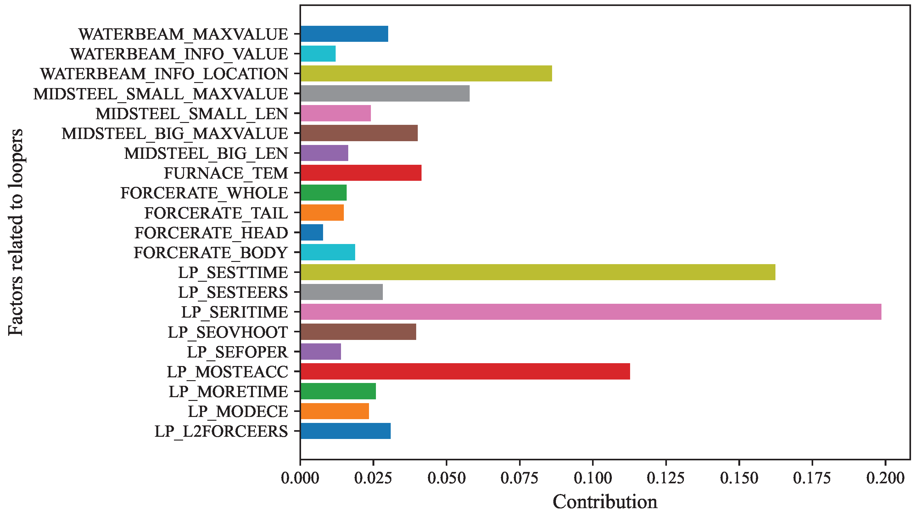
The final result are shown in Figure 10. The factors in the figure are sorted according to their contribution and the factors most likely to cause the looper score to be too low are obtained: LP_SERITIME, LP_SESTTIME, LP_MOSTEACC….
It can be seen from Figure 8 and Figure 10 that in Figure 8 the value of LP_SERITIME (loop servo valve adjustment rising time) is the largest, and in Figure 10 the contribution corresponding to LP_SERITIME is also the highest, and the relationship between the other factors is also very similar, so the algorithm can obtain the correct result. It is not difficult to see that the top three factors with the largest contribution are LP_SERITIME, LP_SESTTIME (loop servo valve adjustment steady-state time), and LP_MOSTEACC (rolling mill speed steady-state error). The above factors have the greatest impact on the low EPAE score of the looper, so these aspects should be prioritized for inspection and maintenance.
We use data from different hot rolling production environments and production lines to verify that the algorithm has excellent generalization ability in different manufacturing environments. When the environment changes, the algorithm can still locate the most likely fault problem. At the same time, even when the algorithm deviates from the initial research conditions, PSO can still obtain the optimal solution for weight calculation through its powerful search ability.
5. Discussion and Conclusions
This paper takes the looper equipment in hot rolling as the starting point, and establishes the EPAE model of the looper based on the control accuracy of the three processes of looping, steady state, and dropping during looper operation. Then, the Pearson correlation coefficient is used to measure the degree of correlation between the EPAE model and specific scenarios of production stability, and a root-cause-tracing algorithm is proposed to locate factor faults. Finally, the data from the 2250 production line is used for testing. The experimental results show that the influencing factors analyzed by this algorithm were consistent with the actual fault factors on site.
The EPAE model proposed in this paper has been applied in many production lines. In addition, the algorithm has been tested in other industrial processes or systems outside the hot rolling production line, such as the chemical industry, to find the reasons for the decrease in chemical production, and has received good results. During the application process, the EPAE model and BP neural network were reconstructed based on the chemical industry’s own process flow and industrial equipment. The final weight calculation method is consistent with this article.
We have received excellent feedback from the Engineering Research Center, when a fault occurs during the hot rolling process this algorithm can accurately identify the underlying issues. In addition, as production continues, the algorithm requires a fixed amount of time to retrain the network, so the feedback has led the iteration of the algorithm towards performing incremental training based on existing data. And the evaluation indicators mainly rely on expert experience to extract and construct. In the future, it can be expanded to other types of production lines and unified index evaluation standards can be established.
Author Contributions
Conceptualization, F.J.; methodology, F.L. and J.G.; validation, Y.S.; formal analysis, J.L. and Z.F. All authors have read and agreed to the published version of the manuscript.
Funding
This research received no external funding.
Institutional Review Board Statement
Not applicable.
Informed Consent Statement
Not applicable.
Data Availability Statement
The data that support the findings of this study are available upon request from the corresponding author.
Acknowledgments
The authors wish to thank the School of Automation and Electrical Engineering of University of Science and Technology Beijing, and National Engineering Research Center for Advanced Rolling and Intelligent Manufacturing of University of Science and Technology Beijing, for supporting research to continue the research work.
Conflicts of Interest
The authors declare no conflicts of interest.
References
- Pittner, J.; Simaan, M.A. An initial model for control of a tandem hot metal strip rolling process. IEEE Trans. Ind. Appl. 2009, 46, 46–53. [Google Scholar] [CrossRef]
- Brengelmans, A.; Jones, T.; Tunstall, J. Dynamic simulation of rolling on a six stand hot strip mill. In IEE Seminar on Tools for Simulation and Modelling; IET: Stevenage, UK, 2000; pp. 3/1–3/6. [Google Scholar]
- Li, X.; He, Y.; Ding, J.; Luan, F.; Zhang, D. Predicting hot-strip finish rolling thickness using stochastic configuration networks. Inf. Sci. 2022, 611, 677–689. [Google Scholar] [CrossRef]
- Song, L.; Xu, D.; Wang, X.; Yang, Q.; Ji, Y. Application of machine learning to predict and diagnose for hot-rolled strip crown. Int. J. Adv. Manuf. Technol. 2022, 120, 881–890. [Google Scholar] [CrossRef]
- Kim, J.; Lee, J.; Hwang, S.M. An analytical model for the prediction of strip temperatures in hot strip rolling. Int. J. Heat Mass Transf. 2009, 52, 1864–1874. [Google Scholar] [CrossRef]
- Liu, Q.; Zhu, Q.; Qin, S.J.; Chai, T. Dynamic concurrent kernel CCA for strip-thickness relevant fault diagnosis of continuous annealing processes. J. Process Control 2018, 67, 12–22. [Google Scholar] [CrossRef]
- Fu, W.; Jiang, X.; Li, B.; Tan, C.; Chen, B.; Chen, X. Rolling bearing fault diagnosis based on 2D time-frequency images and data augmentation technique. Meas. Sci. Technol. 2023, 34, 045005. [Google Scholar] [CrossRef]
- Han, T.; Chao, Z. Fault diagnosis of rolling bearing with uneven data distribution based on continuous wavelet transform and deep convolution generated adversarial network. J. Braz. Soc. Mech. Sci. Eng. 2021, 43, 425. [Google Scholar] [CrossRef]
- Jo, H.N.; Park, B.E.; Ji, Y.; Kim, D.K.; Yang, J.E.; Lee, I.B. Chatter detection and diagnosis in hot strip mill process with a frequency-based chatter index and modified independent component analysis. IEEE Trans. Ind. Inform. 2020, 16, 7812–7820. [Google Scholar] [CrossRef]
- Ding, S.X.; Yin, S.; Peng, K.; Hao, H.; Shen, B. A novel scheme for key performance indicator prediction and diagnosis with application to an industrial hot strip mill. IEEE Trans. Ind. Inform. 2012, 9, 2239–2247. [Google Scholar] [CrossRef]
- Yin, F.C.; Sun, J.; Ma, G.S.; Zhang, D.H. Multivariable decoupling control of hydraulic looper system based on ADAMS-MATLAB Co-simulation. J. Northeast. Univ. (Nat. Sci.) 2016, 37, 500. [Google Scholar]
- Guo, J.; Jia, R.; Su, R.; Zhao, Y. Identification of FIR Systems with Binary-Valued Observations against Data Tampering Attacks. IEEE Trans. Syst. Man Cybern. Syst. 2023, 53, 5861–5873. [Google Scholar] [CrossRef]
- Guo, J.; Wang, X.; Xue, W.; Zhao, Y. System Identification with Binary-Valued Observations Under Data Tampering Attacks. IEEE Trans. Autom. Control 2021, 66, 3825–3832. [Google Scholar] [CrossRef]
- Guo, J.; Diao, J.D. Prediction-based event-triggered identification of quantized input FIR systems with quantized output observations. Sci. China Inf. Sci. 2020, 63, 112201:1–112201:12. [Google Scholar] [CrossRef]
- Choi, I.S.; Rossiter, J.A.; Fleming, P.J. Looper and tension control in hot rolling mills: A survey. J. Process Control 2007, 17, 509–521. [Google Scholar] [CrossRef]
- Militzer, M.; Hawbolt, E.B.; Meadowcroft, T.R. Microstructural model for hot strip rolling of high-strength low-alloy steels. Metall. Mater. Trans. A 2000, 31, 1247–1259. [Google Scholar] [CrossRef]
- Wu, J.; Yan, X. Coupling vibration model for hot rolling mills and its application. J. Vibroeng. 2019, 21, 1795–1809. [Google Scholar] [CrossRef]
- Park, C.J.; Lee, D.M. Input selection technology of neural network and its application for hot strip mill. Ifac Proc. Vol. 2005, 38, 51–56. [Google Scholar] [CrossRef]
- Tan, S.; Liu, J.; Wang, M. Research on the MR-ILQ design method to looper control system in hot strip rolling mills. In Proceedings of the 2010 8th World Congress on Intelligent Control and Automation, Jinan, China, 7–9 July 2010; IEEE: Piscataway, NJ, USA, 2010; pp. 2614–2617. [Google Scholar]
- Ji, Y.; Tian, M.; Guo, P.; Hu, X.; Liu, G. Optimization of Looper Control Systems for Hot Strip Mills. China Mech. Eng. 2017, 28, 410. [Google Scholar]
- Saaty, T.L. The analytic hierarchy process in conflict management. Int. J. Confl. Manag. 1990, 1, 47–68. [Google Scholar] [CrossRef]
- Wu, S.; Fu, Y.; Shen, H.; Liu, F. Using ranked weights and Shannon entropy to modify regional sustainable society index. Sustain. Cities Soc. 2018, 41, 443–448. [Google Scholar] [CrossRef]
- Wang, Y.M. Centroid defuzzification and the maximizing set and minimizing set ranking based on alpha level sets. Comput. Ind. Eng. 2009, 57, 228–236. [Google Scholar] [CrossRef]
- Cohen, I.; Huang, Y.; Chen, J.; Benesty, J.; Benesty, J.; Chen, J.; Huang, Y.; Cohen, I. Pearson correlation coefficient. In Noise Reduction in Speech Processing; Springer: Berlin/Heidelberg, Germany, 2009; pp. 1–4. [Google Scholar]
- Su, C.; Cao, J. Improving lazy decision tree for imbalanced classification by using skew-insensitive criteria. Appl. Intell. 2019, 49, 1127–1145. [Google Scholar] [CrossRef]
- Goh, A.T.C. Back-propagation neural networks for modeling complex systems. Artif. Intell. Eng. 1995, 9, 143–151. [Google Scholar] [CrossRef]
- Li, J.; Cheng, J.H.; Shi, J.Y.; Huang, F. Brief introduction of back propagation (BP) neural network algorithm and its improvement. In Advances in Computer Science and Information Engineering; Springer: Berlin/Heidelberg, Germany, 2012; pp. 553–558. [Google Scholar]
- Elbes, M.; Alzubi, S.; Kanan, T.; Al-Fuqaha, A.; Hawashin, B. A Survey on Particle Swarm Optimization with Emphasis on Engineering and Network Applications. Evol. Intell. 2019, 12, 113–129. [Google Scholar] [CrossRef]
Figure 1.
Hot rolling process.

Figure 2.
Root cause tracing.

Figure 3.
Schematic diagram of looper structure.

Figure 4.
Starting process of the looper.

Figure 5.
Looper factors and self-parameters.

Figure 6.
Self-parameters and looper scoring.

Figure 7.
PSO algorithm.

Figure 8.
Looper factor characteristics of different steel coils.

Figure 9.
The proportion of each factor under multiple experiments.

Figure 10.
Result of root-cause-tracing algorithm.


Table 1.
Factors related to production stability in finishing rolling area.
| Object | Name |
|---|---|
| Control factors | Final temperature hit Plate type Mechanical equipment |
| Material factors | Roll gap setting accuracy Surface quality Electrical equipment |
| Equipment factors | Roll force setting accuracy Width, thickness Water, gas, and thermal equipment |
Table 2.
Evaluation index of process accuracy of the looper.
| Object | Name | Symbol |
|---|---|---|
| Entry process | Starting angle | |
| Rising time | t | |
| Steady-state time | ||
| Steady-state process | Oscillation amplitude | a |
| Number of oscillations | ||
| Looper tension | ||
| Exit process | Falling time | |
| Steel-throwing tension | ||
| Small set time | ||
| Small set angle |
Table 3.
Process accuracy evaluation and finish rolling stability.
| Equipment | Correlation Coefficient | p-Value |
|---|---|---|
| Side Guide | −0.768 | 4.087 × |
| Looper | −0.113 | |
| Automatic Gauge Control | −0.458 | |
| Bending Roller | −0.855 | 6.627 × |
| Shifting Roller | −0.356 |
Table 4.
Looper corresponding factor table.
| Serial Number | Looper Corresponding Factors |
|---|---|
| 1 | LP_L2FORCEERS |
| 2 | LP_MODECE |
| 3 | LP_MORETIME |
| 4 | LP_MOSTEACC |
| 5 | LP_SEFOPER |
| 6 | LP_SEOVHOOT |
| 7 | LP_SERITIME |
| 8 | LP_SESTEERS |
| 9 | LP_SESTTIME |
| 10 | FORCERATE_HEAD |
| 11 | FORCERATE_BODY |
| 12 | FORCERATE_TAIL |
| 13 | FORCERATE_WHOLE |
| 14 | FURNACE_TEM |
| 15 | MIDSTEEL_BIG_LEN |
| 16 | MIDSTEEL_BIG_MAXVALUE |
| 17 | MIDSTEEL_SMALL_LEN |
| 18 | MIDSTEEL_SMALL_MAXVALUE |
| 19 | WATERBEAM_INFO_LOCATION |
| 20 | WATERBEAM_INFO_VALUE |
| 21 | WATERBEAM_MAXVALUE |
Table 5.
Neural network parameter settings.
| Parameter | Value |
|---|---|
| Input layer node | 21 |
| Middle layer node | 7 |
| Output layer node | 2 |
| Activation function | Sigmoid function |
| Error back-propagation | Derivative of sigmoid function |
| Threshold | 0 |
| Loss function | Mean square error function |
Table 6.
PSO parameters.
| Parameter | Setting Value |
|---|---|
| 0.8 | |
| 0.5 | |
| 0.5 | |
| Upper bound | 1 |
| Lower bound | 0 |
| Number of particles | 50 |
| Number of iterations | 1000 |
| Tensor | 21 |
Table 7.
The iterative process of using PSO to solve the system of equations.
| Test Serial Number | Largest Proportion | Second Proportion | Third Proportion |
|---|---|---|---|
| 1 | LP_SERITIME 0.1926 | LP_SESTTIME 0.1670 | LP_MOSTEACC 0.1156 |
| 2 | LP_SERITIME 0.1912 | LP_SESTTIME 0.1678 | LP_MOSTEACC 0.1144 |
| 3 | LP_SERITIME 0.1896 | LP_SESTTIME 0.1668 | LP_MOSTEACC 0.1107 |
| 4 | LP_SERITIME 0.1870 | LP_SESTTIME 0.1681 | LP_MOSTEACC 0.1116 |
Disclaimer/Publisher’s Note: The statements, opinions and data contained in all publications are solely those of the individual author(s) and contributor(s) and not of MDPI and/or the editor(s). MDPI and/or the editor(s) disclaim responsibility for any injury to people or property resulting from any ideas, methods, instructions or products referred to in the content. |
© 2024 by the authors. Licensee MDPI, Basel, Switzerland. This article is an open access article distributed under the terms and conditions of the Creative Commons Attribution (CC BY) license (https://creativecommons.org/licenses/by/4.0/).
Share and Cite
MDPI and ACS Style
Jing, F.; Li, F.; Song, Y.; Li, J.; Feng, Z.; Guo , J. Root Cause Tracing Using Equipment Process Accuracy Evaluation for Looper in Hot Rolling. Algorithms 2024, 17, 102. https://doi.org/10.3390/a17030102
AMA Style
Jing F, Li F, Song Y, Li J, Feng Z, Guo J. Root Cause Tracing Using Equipment Process Accuracy Evaluation for Looper in Hot Rolling. Algorithms. 2024; 17(3):102. https://doi.org/10.3390/a17030102
Chicago/Turabian StyleJing, Fengwei, Fenghe Li, Yong Song, Jie Li, Zhanbiao Feng, and Jin Guo . 2024. "Root Cause Tracing Using Equipment Process Accuracy Evaluation for Looper in Hot Rolling" Algorithms 17, no. 3: 102. https://doi.org/10.3390/a17030102
Note that from the first issue of 2016, this journal uses article numbers instead of page numbers. See further details here.