
Progressive Multiple Alignment of Graphs


1
Bioinformatics Group, Department of Computer Science, Interdisciplinary Center for Bioinformatics, Leipzig University, Härtelstraße 16-18, D-04107 Leipzig, Germany
2
Center for Scalable Data Analytics and Artificial Intelligence (ScaDS.AI), Leipzig University, D-04103 Leipzig, Germany
3
Max Planck Institute for Mathematics in the Sciences, Inselstraße 22, D-04103 Leipzig, Germany
4
Department of Theoretical Chemistry, University of Vienna, Währingerstraße 17, A-1090 Vienna, Austria
5
Center for Non-Coding RNA in Technology and Health, University of Copenhagen, DK-1870 Fredriksberg, Denmark
6
Facultad de Ciencias, Universidad National de Colombia, Sede Bogotá, Bogotá CO-111321, Colombia
7
Santa Fe Institute, 1399 Hyde Park Rd., Santa Fe, NM 87501, USA
*
Authors to whom correspondence should be addressed.
Algorithms 2024, 17(3), 116; https://doi.org/10.3390/a17030116
Submission received: 19 January 2024
/
Revised: 21 February 2024
/
Accepted: 7 March 2024
/
Published: 11 March 2024
(This article belongs to the Special Issue Graph Algorithms and Graph Labeling)
Abstract
:The comparison of multiple (labeled) graphs with unrelated vertex sets is an important task in diverse areas of applications. Conceptually, it is often closely related to multiple sequence alignments since one aims to determine a correspondence, or more precisely, a multipartite matching between the vertex sets. There, the goal is to match vertices that are similar in terms of labels and local neighborhoods. Alignments of sequences and ordered forests, however, have a second aspect that does not seem to be considered for graph comparison, namely the idea that an alignment is a superobject from which the constituent input objects can be recovered faithfully as well-defined projections. Progressive alignment algorithms are based on the idea of computing multiple alignments as a pairwise alignment of the alignments of two disjoint subsets of the input objects. Our formal framework guarantees that alignments have compositional properties that make alignments of alignments well-defined. The various similarity-based graph matching constructions do not share this property and solve substantially different optimization problems. We demonstrate that optimal multiple graph alignments can be approximated well by means of progressive alignment schemes. The solution of the pairwise alignment problem is reduced formally to computing maximal common induced subgraphs. Similar to the ambiguities arising from consecutive indels, pairwise alignments of graph alignments require the consideration of ambiguous edges that may appear between alignment columns with complementary gap patterns. We report a simple reference implementation in Python/NetworkX intended to serve as starting point for further developments. The computational feasibility of our approach is demonstrated on test sets of small graphs that mimimc in particular applications to molecular graphs.
1. Introduction
The notion of alignments was introduced as a means of sequence comparison in computational biology [1]. Pairwise sequence alignments can be understood as representations of solutions to the string-editing problem, in which one string is converted into another one by a minimal sequence of insertions, deletions, and substitutions. Letters missing in a sequence are denoted by a special gap character “-”. The notion easily generalizes to alignments of more than two sequences, resulting in a matrix whose rows correspond to the input sequences (padded by gap characters) and whose columns designate corresponding letters, i.e., homologous characters in applications to biological sequences; see [2] for a detailed review. The concept of alignments was later extended to rooted ordered trees [3] as a means of comparing RNA secondary structures [4]. More recently, a formal framework was developed to define alignments in a much more general setting [5], which we will review in the Theory section below (Section 2) in some detail. In this general setting, alignments are considered as super-objects containing the contributing input objects (sequences, trees, graphs, etc.) such that these are recovered by means of well-defined projections. Specializing this framework to graphs yields a notion of multiple graph alignment (MGA) that pertains to both directed and undirected graphs and also accommodates labeled graphs. The key property of an MGA is that the constituent input graphs appear as induced subgraphs of the alignment graph.
The term “graph alignment” is frequently used in the literature to refer to matchings between the vertex sets of graphs that maximize some similarity measure [6,7,8]. The construction considered in [9] uses “alignment” columns allowing “dummy nodes” corresponding to gap symbols, but does not endow the “alignment” with a graph structure. Similarly, IsoRank in its 1-1 mapping mode [10] computes a maximum weighted multipartite matching between the vertices of input networks constrained in such a way that the connected components of its transitive closure (i.e., the alignment columns) contain at most one vertex from each of the . The weights are application-specific similarity scores computed for all pairs of vertices from different and typically combine similarities of vertex attributes with neighborhood similarities, as in FINAL [11] or HashAlign [12]. Different algorithmic approaches have been employed to solve this optimization problem. While [10] uses a greedy heuristic, integer quadratic programming is proposed in [13]. Moreover, a wide variety of learning approaches have been used in recent years for this type of graph comparison, see, e.g., [14] and the references therein.
In summary, all these graph matching methodologies differ in two important aspects from the concept of alignments used here: (1) they do not require the strict preservation of the local structure inherent in alignments and (2) they do not consider the alignment again as a graph. Furthermore, in [15], a “graph alignment” was defined by means of injective embeddings of the input graphs into an “entity graph” H such that vertices adjacent in are mapped to adjacent vertices in H. In contrast to our framework, however, non-adjacent vertices in may be mapped to adjacent vertices in H. The constituent graph thus appears as subgraphs of H but not induced subgraphs of H and thus is not recoverable from H as a projection.
The compositional properties of alignments [5] require both the projective property and the fact that the alignment is again a graph. As a consequence “alignments of graph alignments” are well defined, preserve the projections of the constituent input graphs, and thus are again graph alignments of the same constituent graphs. This is a prerequisite for introducing the notion of a progressive graph alignment guided by a similarity tree (Section 3.1), in analogy to the progressive methodologies employed for multiple sequence alignment [16]; for an overview of our methodology, see Figure 1. Graph matchings, in contrast, have much weaker compositional properties. As noted in [9], pairwise graph matchings with a common “reference graph” can be combined to a matching of multiple graphs. On the other hand, in our setting, alignments of graph alignments can be combined arbitrarily. The compositional properties of the construction in [15], which lacks the projective property, have not been studied to our knowledge. Graph matching approaches, including [15], thus address combinatorial optimization problems that are clearly distinct from the formal graph alignments studied here.
The multiple alignment problem is NP-complete already for sequences [17,18,19]; hence, in practice, one has to resort to heuristics. A simple but efficient approach are progressive alignments [16], which reduce the problem to computing pairwise alignments of alignments of subsets of input objects. Progressive multiple alignments of rooted ordered forests have been considered in [4] as means of comparing multiple RNA structures. Star alignments, comprising the pairwise alignments of all input objects to common reference objects, are related to progressive alignments. This strategy has been explored in [9] for graph matchings. For large networks, an evolutionary algorithm [20] and an ant-colony algorithm [21] have been explored.
Here, we describe a progressive alignment procedure that is based on exact pairwise graph alignments. As we shall see, these can be computed from maximum common induced subgraphs (MCISs). To this end, we first introduce the formal theory of multiple alignments of graphs that properly generalizes sequence alignments. We then demonstrate that MGAs can be computed with a progressive framework in practice and show that this approach yields accurate results. Since we consider here an optimization problem that is significantly different from graph matching approaches considered in the literature, we refrain from comparing MGAs with graph matching methods.
![Algorithms 17 00116 g001]()
Figure 1.
Overview of the ProGrAlign to compute a multiple graph alignment of a collection of input graphs (a). A fast heuristic, here using a graph kernel, is used to determined pairwise similarities between the input graphs. The similarity matrix (b) is used to construct a guide tree (c) using a clustering method such as WPGMA [22]. This guide tree dictates the order in which one is to compute pairwise alignments. Alignments of graphs, e.g., of and , are again graphs. Thus, alignments of alignments with other input graphs, here , or graph alignments, are well defined and reduced to computing pairwise graph alignments. The final result is obtained as the alignment corresponding to the root of the guide tree. (d) Every input graph is contained in the multiple alignment graph as an induced subgraph, emphasized here with darker vertices and edges.

Our contribution is organized as follows: In Section 2.1, we derive MGAs as a specialization of the abstract framework of alignments as super-objects, thereby streamlining some key ideas of [5]. Section 2.2 introduces the new concept of ambiguous edges, which leads us in Section 2.3 to a complete characterization of pairwise graph alignments. Moreover, we clarify the relationship of the alignment supergraphs with the maximum common induced subgraphs playing the role of matches. On this basis, we formally introduce progressive MGAs in Section 2.4. The remaining two theory subsections are dedicated to the alignments of labeled graphs and show that for monotone scoring functions, pairwise graph alignments can be computed exactly from maximum common induced subgraphs. Section 3 is concerned with a practical implementation of progressive MGAs. Section 3.1 describes the construction of a guide tree. In Section 3.2, we describe the adaptation of VF2-like algorithms [23,24] for our purposes. In more detail, we describe the proper incorporation of ambiguous edges in Section 3.3. The implementation of a proof-of-concept software tool is described in Section 4. In addition to studying the influence of algorithmic parameters, we describe the influence of the diversity of the input dataset. Additional details are described in Appendix A. We introduce consensus graphs as a specific application in Section 4.3. We conclude with a short discussion of our contributions and open questions.
2. Theory
2.1. Abstract Graph Alignments
Following [5], we consider a class of finite hereditary set systems , where X is a finite set and is some subset of such that for every subset the restriction of to Y is well defined and satisfies the following consistency property for all . In the following, we will refer to as an object. For , will be called the subobject of X induced by Y. Two set systems and are isomorphic if there is a bijection such that , where we use the convention that the application of a function to a set is defined point-wise, i.e., . In this case, is an isomorphism and we write .
A very simple example of an object is the set X of positions in an DNA or protein sequence endowed with the total order ≤ since these linear biomolecules have a specified orientation. The subobjects of are obtained as subsets of that preserve the order. To see that this indeed conforms to the abstract set systems introduced in the previous paragraph, we note that order relations can be encoded by sets: Setting we see that if and only if . Thus the order ≤ is encoded by the subset relation in the set system . The subobjects induced by Y thus are the set systems . Similarly, we may consider the class of rooted ordered trees [3]. As noted, for example, in [5], these correspond to finite sets with an orthogonal pair of partial orders: two vertices are either equal, comparable w.r.t. to the ancestor order, or w.r.t. to sibling order. In the present contribution, the objects of interest are graphs. Here, X denotes the vertices and corresponds to the edges of a graph, i.e., is a set of unordered pairs of distinct vertices. The sub-objects are the induced subgraphs defined by a subset of vertices.
Abstractly, an alignment of a set of “input” objects consists of an object of the same class that contains each of the . More precisely, is contained in X in the sense that there is an injective function such that the subobject where is isomorphic to with being an isomorphism.
It will be convenient to think of the as the rows of the alignment in analogy to multiple sequence alignments. Correspondingly, each specifies a column. Thus, the alignment can be encoded by a pair where and each component determines a subset such that
To avoid trivial cases, we forbid “all-gap columns”, i.e., we insist that for at least one i. Since we assume that the induced subobjects are unique, f defines the embeddings up to isomorphism.
We say that a point x in an alignment corresponds to a match column of for all i. Writing for the set of matches, we observe that the restriction of to is a common sub-object of all . The converse is not always true; however, it is not always possible to extend a common sub-object to an alignment that contains a common sub-object such as the set of matches. Probably the most well-known example is the distinction between the editing and alignment of two rooted ordered forests, see (e.g., [25] Figure 1).
In the case of graphs, however, the situation is simple. Let G and H be two graphs with a common induced subgraph K with embeddings and . Identifying the vertices and for all amounts to gluing together G and H at the vertices of K. This results in a graph A that contains K as an induced subgraph. All other vertices belong to either or . By construction, A contains only edges that are present in at least one of G and H, and both G and H are contained in A as induced subgraphs. In particular, therefore, A is an alignment of G and H. It is, in fact, the unique edge-minimal alignment of G and H given the common induced subgraph K.
2.2. Ambiguous Edges
The alignment A of G and H is, however, not the only possible alignment of the two graphs G and H. While every common induced subgraph defines a unique edge-minimal alignment, it is possible to find alternative graphs that are also valid alignments of G and H. To see this, let G be an alignment of . An edge of G is present in the projection if and only if and . An edge in G thus never appears in any of the input graphs if and only if for all i, i.e., if its two incident vertices never appear together in the same input graph. We call such edges ambiguous edges.
It is not difficult to identify the ambiguous edges in a pairwise graph alignment: an ambiguous edge exists between all pairs of vertices from different input graphs that are not part of a common induced subgraph. More formally, the set of ambiguous edges comprises all (unordered) pairs with and . Given a common induced subgraph K of G and H, a graph is an alignment of G and H with match columns defined by K if and only if its edge set satisfies .
2.3. Characterization of Pairwise Graph Alignments
An immediate consequence of the theory outlined above is the following characterization of the set of pairwise alignments of two input graphs G and H:
A graph A, is a graph underlying an alignment of two graphs G and H, if and only if, A is is obtained by “gluing together” G and H along a subgraph-isomorphism embedding a common induced subgraph K into G and H, and adding an arbitrary subset of ambigous edges, i.e, with one endpoint in and the endpoint in .
This characterization extends the one given in [26] by accommodating ambiguous edges. Hence, for every common induced subgraph K, there is a unique edge-minimal pairwise alignment, characterized by the absence of ambiguous edges. Similarly, for a given K, the edge maximal alignment is uniquely defined by inserting all ambiguous edges. Two alignments are distinct if K or the embedding of K into G and H differs. This observation provides, in principle, a means of enumerating all possible alignments of two input graphs.
It is worth noting, finally, that there does not seem to be a simple generalization of this statement to multiple alignments of graphs. The reason is that the matches between multiple graphs need to satisfy consistency conditions that arrange them into alignment columns. Apart from order preservation, which is replaced by adjacency preservation in our case, these conditions are the same as for sequence alignments [27].
2.4. Progressive Alignments
Consider an alignment and let be a bipartition of the set S of rows, i.e., , , and . Furthermore, let and . Consider the restriction of the sub-object to the rows for . Then , is an alignment of the input objects with and can be seen as a pairwise alignment of and . For the full formal details, we refer to [5]. As a consequence, every alignment can be recursively subdivided into alignments of bipartitions of its rows. Since every input object is itself a (trivial) alignment, this decomposition yields a rooted tree T whose leaves are input objects , whose root is the alignment , and whose interior nodes correspond to alignments of certain subsets of input alignments.
The idea of progressive alignment algorithms is to construct an alignment from the input objects along a binary guide tree T such that at each inner node, a pairwise alignment of the alignments associated with its children are computed (Figure 2). The compositionality properties ensure this is always possible, irrespective of how the tree T is chosen and how the pairwise alignments are computed in practice [5]. Here, we construct a progressive alignment algorithm for graphs. Clearly, for each interior node of an arbitrary binary guide tree, it suffices to find a maximum common induced graph and use it to determine how to glue the two child-graphs together. Note that at this point, we make no statement on the optimality of the either or any of the intermediates. We merely state that every graph alignment can be obtained by reverting the process of its decomposition along any binary tree T. Ambiguous edges only provide a moderate complication in progressive alignments, which we will consider below in conjunction of the scoring model. In fact, when extending a set of matches, one can choose whether an ambiguous edge is considered to be present or absent.
2.5. Labels
Usually, the input objects are endowed with a labeling function , where L is a finite set of labels. For biological sequence alignments, denotes the nucleotide or amino acid at sequence position . Similarly, if the graphs designate structural formulae of organic molecules, then is the chemical element of atom x in molecule . Often, alignments are specified directly in terms of these labels. Thus, we may set such that if and if . The gap symbols - therefore correspond exactly to the points (i.e., alignment columns) in X that are deleted in . Since we have if and if , we can equivalently specify the alignment by . The labeled input objects are thus obtained from by deleting from X all vertices with and retaining, on the i-th label, for all other points.
The labels can be used to impose additional constraints on the common sub-objects. For instance, one may want to restrict matches to vertices with same labels, in which case and implies . This is useful, e.g., to preserve atom labels. In principle, arbitrary rules for the (in)compatibility of labels in a column can be defined.
2.6. Labels and Scores for Graph Alignments
Labels are in particular used to introduce scoring functions, such as the BLOSSUM scores for (mis)matches of amino-acids. Most commonly, these are defined for pairwise alignments. Since all our practical computations also will involve only pairwise alignments, it suffices to consider the issue of scoring also for the pairwise case only.
In this case, a common subobject is specified by a set of matches M whose elements are pairs with and . Since the restriction of a set of matches to a subset is again a set of matches and thus defines again a common sub-object, the set of all sets of matches forms an independence system, i.e., and implies . We shall consider here only scoring functions that are defined on sets of matches, i.e., the score of a pairwise alignment is given by where M is the set of matches corresponding to match columns .
We say that a scoring function is strictly monotone if implies . For strictly monotone scoring function, the maximum score can be attained only for sets of matches that are maximal, i.e., that cannot be augmented by an additional match. In the case of graphs, furthermore, every set of matches defines an alignment (which is unique up to ambiguous edges), and thus an optimal alignment is determined by a MCIS that in addition maximizes the scoring function . The score may also depend on edge labels within the common induced subgraphs as long as the strict monotonicity property is preserved.
A convenient special case is an additive scoring scheme in which every vertex-match and every edge-match yield a non-negative contribution. The inclusion of additive edge-dependent scores is unproblematic from an algorithmic point of view because any procedure that adds or removes a match also adds or removes the incident edges connecting to the vertices in the rest of the common induced subgraph. Thus, every edge in the common induced subgraph is associated with a unique vertex operation, ensuring that adding/removing of single vertices affects the total score in a consistent manner.
Assuming a strictly monotone scoring model, ambiguous edges are easy to handle. Suppose we attempt to add a match to a set M of matches. Then, the edge to some match is added if either both and are ambiguous edges, or one of the two edges is unambiguous and the other is ambiguous. No edge is inserted if there is a non-edge between and or and . Note that if both the edges and are ambiguous, then is again ambiguous. In either case, the extension of M by by assumption incurs a positive score increment and thus yields a better score than leaving and as two unmatched vertices. Finally, we note that since ambiguous edges are removed in all branches at some lower-down node of the guide tree, they do not convey information on the input graphs. Thus, an edge where or is ambiguous naturally does not yield a positive score even when otherwise edge-matches are associated with score contributions.
The most natural scoring function for alignments of alignments is the sum-of-pairs scoring model, in which the contributions of all pairwise alignments are simply added. In our setting, this is particularly appealing since gap characters (−) simply do not contribute to the scoring at all. Note that the sum-of-pair scoring also preserves strict monotonicity, since each extending match by construction yields non-zero contributions for at least one row in each of the aligned alignments.
3. Algorithmic Considerations
3.1. Construction of the Guide Tree Based on Graph Kernels
Every binary tree with leaves that are in a one-to-one correspondence with the input graphs may serve as guide tree for a progressive alignment. It is well known for multiple alignments of sequences, however, that the guide tree influences the quality of the alignment [28,29]. In the case of graph alignments, the computational effort for computing MCIS, and thus for the pairwise alignment problems, also depends on the similarity of the input graphs. It is desirable, therefore, to use a guide tree along which for each inner node, the two children correspond to graphs that are as similar as possible. The most useful guide trees thus correspond to a parsimonious hierarchical clustering of the input graphs [16]. In the case alignments of homologous genetic sequences, a good approximation of the correct phylogeny is ideal. In practice, good guide trees are obtained by hierarchical clustering of the input objects.
The progressive computation of the multiple alignment requires pairwise alignments. In contrast, all pairwise comparisons are required for hierarchical clustering to estimate the guide tree. However, pairwise alignments can be used to compute the distances or similarities of all pairs of input objects. It is therefore desirable to replace the alignment-based similarities by a computationally less expensive approximation for the computation of the guide tree. Comparisons of two graphs based on MCIS [30], i.e., , as well as other forms of graph editing distance [31] are NP-complete.
Among the heuristic alternatives are distance measures based on semi-definite graph kernels [32], i.e., bilinear functions on a non-empty set satisfying for all and any . The kernel function in essence provides a similarity measure between graphs.
Furthermore, as shown in [33,34], due to its relation with inner products in vector spaces, the similarities can be transformed into a distance measure by taking the square root of the value . Both the similarities and its associated distances can be used as inputs for a simple agglomerative hierarchical clustering procedure, here simply WPGMA [22], to infer a guide tree .
Originally conceived in cheminformatics, a wide array of graph kernels has been studied depending on different properties and features of graphs, including paths, walks, cycles, spanning trees, matchings, local subgraphs, etc.; see [35] for a survey. Implementations of kernel functions for graphs (including labeled, weighted, and directed graphs) are available as widely used software packages such as graphkit-learn [36]. Here, we made use of the Structural_Shortest_Path kernel implementation of the graphkit-learn library in order to produce our kernel-based guide trees. As shown in Appendix A.1, the kernel-based distance and the MCIS-based distance are well correlated.
3.2. Computing Optimal Common Induced Subgraphs
As discussed in Section 2.6, optimal pairwise alignments are based on score-optimal common induced subgraphs, which in turn are maximal common induced subgraphs. Computing MCIS is known to be computationally hard. The corresponding decision problem is NP-complete [37] and hard to approximate [38]. For small graphs with limited degree and non-trivial labels, such as in particular molecule graphs, it is nevertheless feasible to solve MCIS exactly. Probably the best known algorithmic approach is to compute the modular product of using the fact that an MCIS of G and H corresponds to a maximum clique in [39]. It is not obvious, however, how ambiguous edges can be handled efficiently in this setting.
The main alternative is a class of search procedures based on the step-wise extension of a matching by candidate matches with and . These algorithms are designed for the subgraph isomorphism problem, i.e., to recognize whether the smaller of the two input graphs, , is isomorphic to an induced subgraph of the larger one, , [23,24]. Starting from the empty set of matches, this yields a search tree whose leaves are the maximal induced common subgraphs. A positive answer to the subgraph isomorphism problem corresponds to a leaf in which is matched in its entirety. McSplit and similar algorithms combine the extension of M with bounds on the number of possible extending matches in order to obtain a full-fledged branch-and-bound approache [40,41,42]. It is not clear, however, how good bounds can be obtained in the presence of ambiguous edges and arbitrary compatibility rules for the labels of vertices and edges. Our implementations thus focus on the enumeration of maximal common induced subgraphs.
In order to accommodate prior knowledge, it is sometimes of interest to compute alignments that incorporate an anchor, i.e., set of matches that are given as part of the input. For sequence alignments, this idea has been explored, e.g., in CONREAL [43] and an anchored version of dialign, both with applications of phylogenetic footprinting [44]. The idea of anchors generalizes to graph alignments in a straightforward manner. Instead of starting from an empty set of matches , we can insist that any valid set of matches M contains the anchor matches, . This is trivially enforced in VF2-like approaches, where anchors lead to a drastic reduction in the search space since only the subtree rooted at the anchor matches needs to be processed.
If the MCIS is expected to be small compared to both and , then a direct, VF2-like expansion of the matches set M appears to be the most promising strategy. If the solution is expected to cover most of , a viable alternative is to “trim” by removing some of its vertices; see Algorithm 1. An optimized subgraph isomorphism test, denoted by VF2_sgi in Algorithm 1, can then be used to decide whether the trimmed induced subgraph of appears as a subgraph in . This allows us to use many of the optimizations in VF2 that are not applicable if all maximal common subgraphs need to be enumerated. The iteration over the sets S of removed vertices can be restricted to terminate at the cardinality at which the first match M is encountered as in our current implementation. While a recursive version of such a trimming algorithm could also be implemented, it seems difficult to make use of latter bound in such a setting. Alternatively, it may exclude S if a non-empty set of matches was returned already for one of its subsets. We note that for arbitrary monotone scores, the latter strategy must be employed since there is no guarantee that the MCIS with the maximum score is also maximum in cardinality.
| Algorithm 1: Iterative_Trimming |
 |
The basic step of the VF2-like approach is formalized in Algorithm 2. To compute the MCIS of and with a possibly empty set of anchor matches, one calls VF2_step(). The end result is the set of all maximal matchings containing that correspond to a maximal common induced subgraph. During the recursive traversal of the search tree, a set of extension candidates P is computed for a the current matching M. If M cannot be extended, i.e., if there is no compatible match for M, then M forms a leaf in the search tree and is added to result set . Assuming a strictly monotone scoring function, the set of matches of a score-maximal pairwise alignment is necessarily maximal w.r.t. cardinality [30,45]. It therefore suffices to evaluate the scores of the matchings M at the leaves of the search tree constructed by VF2_step.
The computation of the candidate matches, Algorithm 3, depends on a fixed total order of the vertices of the smaller graph . In order to avoid the duplication of branches in the search tree, only matches of vertices in following all vertices in matches of M, except those of a possible anchor, are considered. It is convenient to choose the order such that the vertices in that are part of the anchor are numbered .
The routine VF2_sgi in Iterative_Trimming is similar to VF2_step, except for further heuristic optimizations to speed up the decision of whether is isomorphic to a subgraph of or not. The implementation of both routines is adapted to handle ambiguous edges and comparing vertex and edge labels when requested by the user, and can be set to optimize a monotone scoring function instead of the number of vertices in the MCIS as well.
| Algorithm 2: VF2_step |
 |
| Algorithm 3: candidate_matches |
Data: Graphs and a matching Result: Set P of match candidates for extending M set of unmatched vertices in set of unmatched vertices in // the anchor is contained in M and would be excluded from the candidates return
P |
The original formulation of the VF2 algorithm differs from our adaptation VF2_step for MCIS-search by using a different algorithm candidate_matches for proposing candidates for matches that extend M. The version used in VF2 is optimized to determine whether H is isomorphic to a subgraph of G by restricting the candidates to combinations of unmatched neighbors of and of for every match , provided such vertices exist. This restriction, however, makes the assumption that it is possible to extend the matching M as long as there are still unmatched vertices in connected components that contain vertices in M. This is true if H is isomorphic to a subgraph of G (or vice versa), but fails for the MCIS search. A detailed example showing that the standard implementation of VF2 can fail to find an MCIS is given in Appendix A.2. The candidate search used by VF2_sgi inside Iterative_Trimming is the same in the original VF2 approach.
3.3. Syntactic and Semantic Compatibility
The compatibility test compatible operates in two stages:
Syntactic compatibility requires, for each , that and preserve adjacency. For the pairwise alignment of graphs, syntactic compatibility is straightforward because there are no ambiguous edges: is syntactically compatible with M if and only if, for every , either both and are not adjacent or both and . At this stage, ambiguous edges need to be handled.
Semantic compatibility requires that vertex labels are allowed to be aligned according the user-defined evaluation scheme. We denote by and the labels of vertices and edges. In general, the labels of vertices and edges in an alignment graph, i.e., and for alignment columns x and y, are multisets of “elementary” labels defined on the input graphs, i.e., rows of the alignment. In general, the labels and are multisets of “elementary” labels defined on the input graphs. Moreover, we assume a relation that defines when two elementary vertex labels or two elementary edge labels are compatible. This pairwise compatibility rule can be chosen arbitrarily by the user. For alignments of alignments, label sets are compatible if and only if all pairs of labels are compatible, where gaps − are assumed to be compatible with all labels.
In order to keep track of ambiguous edges, it is useful to consider a tri-partitions of into unambiguous edges E, unambiguous non-edges Q, and ambiguous edges A. For simplicity, we write for the matching edges.
Since semantic consistency in our setting is defined exclusively in terms of vertex and edge labels, the semantic filter can, in principle, be integrated with the syntactic consistency check. The discussion in the theory section immediately implies that a matching M is consistent if and only if:
- (a)
- the two vertex labels and the two vertex labels are compatible and
- (b)
- for all one of the following conditions is satisfied:
- (i)
- and and the two edge labels and are are compatible, or
- (ii)
- and , or
- (iii)
- or .
Clearly, the three conditions (i), (ii), and (iii) are mutually exclusive. Moreover, if M is consistently matching and is a candidate for extension, then is consistent if and only if the and are compatible and for every , one of the conditions (i), (ii), or (iii) is satisfied. Since each of the three conditions can be checked in constant time, testing whether M can be extended by requires time.
These relationships immediately generalize to directed graphs: compatibility condition (i) then requires that also the direction of the edges matches, i.e.,
- (i’)
- If and are connected by directed edges, then iff and the labels of these directed edges, and , are compatible.
Ambiguous edges, on the other hand, are consistent with all edge directions and edge labels, as well as the absence of an edge. For a consistent matching M, the corresponding graph and its ambiguous edges are uniquely defined by M as follows: In case (i), we have . In case (ii), we have . In case (iii), we have to distinguish the following cases:
- (1)
- If and , or and , then ;
- (2)
- If and , or and , then ;
- (3)
- If and , then .
Again, can be constructed from is given with effort. The generalization to directed graphs is straightforward: In cases (2) and (3), the direction of the edge(s) in the alignment is defined by the edges in either or , respectively.
Since we store the binary vector for each alignment column x, it is not necessary to explicitly store the sets E, Q, and H. Instead, it suffices to store the unambiguous edges E and to use if and only if , where ⊙ denotes component-wise binary multiplication.
3.4. Visualization of Alignment Objects
Sequence alignments can be visualized as a rectangular matrix, with rows corresponding to the input sequences. In the case of graph alignments, the matrix representation, shown in Figure 3, is also suitable to show the correspondence of vertices.
It should be noted, however, that the order of the vertices is arbitrary unless one considers graphs with a fixed vertex order as in the case of contact graphs for RNA or protein structures [26]. Moreover, this kind of matrix representation contains no information of the graph structure.
Alternatively, one starts from a planar layout of the alignment graph G. Since every input graph is an induced subgraph of G, an embedding of can be obtained by retaining only vertices and edges of . As shown in Figure 3, spatial correspondence of the layouts emphasizes the embedding of in G.
Still, this representation is not always easy to read. An improvement is obtained by superimposing the embeddings of the input graphs in stacked planes above the embedding of G such that each set of aligned vertices lies on a common vertical line (Figure 4). Coloring the vertices depending on their position in G further improves readability.
4. Computational Results
4.1. Implementation
As a proof of concept, we developed the Progressive Graph Alignment toolkit ProGrAlign in Python language, making extensive use of the NetworkX [46], a library that is widely used for graph analysis. ProGrAlign is publicly available in a Github repository [47]. It consists of three software tools: ProGrAlign_Analysis computes the progressive graph alignment using a list of graphs built as NetworkX objects. The graphs can be undirected, directed, labeled or weighted, and may have loops. It is necessary that either all input graphs are undirected or all input graphs are directed. Functions to convert undirected graphs into symmetric directed graphs, or directed graphs into their underlying undirected graphs, are readily available in NetworkX. Input and output use the binary files produced with the Pickle [48] standard package for the serialization of Python objects. Additionally, two visualization tools are provided, ProGrAlign_Vis2D and ProGrAlign_Vis3D, which make use of the Matplotlib [49] library to display the alignment graph.
4.2. Generation of Test Sets
Alignments of graphs are useful, in particular if one expects them to be derived from a common source by means of a process that introduces small or moderate variations. This is, in particular, the case for evolutionary processes in a biological setting, but also in the case of repeated noisy measurements of interactions or in a setting such as social networks that change over time. In order to demonstrate and benchmark our implementation, we therefore also developed a simple random-graph model that produces “mutant graphs” along an evolutionary tree.
The tool first generates an initial graph with the gnm_random_graph generator provided by NetworkX [46], a Python library for graph analysis. This model produces a graph having n vertices and exactly m edges chosen uniformly at random from all the possible edges between these vertices. To avoid trivial cases, we require, in addition, that is connected, which can also be iteratively verified and enforced with the functionalities included in NetworkX. Labels are then assigned independently to vertices, and edges drawn form a uniform distribution over finite label sets. For the example below, we choose five distinct labels for both vertices and edges.
The mutation operator acting over a connected graph G first deletes one or two vertices, such that G remains connected, and then adds one or two vertices and inserts, where for each of them, a number of edges is chosen uniformly from the degree sequence of G. If two vertices are added, one may be chosen as a neighbor of the other during edge addition. The creation of loops is not allowed. Random labels are then associated with the new vertices and new edges.
The set of test graphs is produced by applying the mutation operator along a planted rooted binary tree rooted by . The single child of has two children and , and four grandchildren to . Again, we exclude trivial examples by requiring connectedness and removing graphs that by chance are isomorphic to a previously generated one. Standard functions provided by NetworkX are used for this purpose. Starting with 16 vertices at , the graphs , have between 13 and 19 vertices. All tests are preformed with 50 independent sets of test graphs.
4.3. Consensus Graphs
An important motivation for graph alignments is consensus graphs generalizing the idea of consensus sequences [50] and consensus forests [4]. Given an alignment graph , a consensus graph is obtained as an induced subgraph of with a vertex set W obtained from the gap pattern function by means of a voting procedure. In the simplest case, the vertex set comprises all alignment columns with a sufficient fraction of non-gap entries. Vertex and edge labels for W and , resp., can also be obtained with the help of suitable voting procedure. A key property of consensus sequences is that they approximate the ancestral state or the master sequence of viral quasi-species. Consensus sequences also are of use, e.g., to determine an accurate genome or transcript sequence from a set of noisy sequencing reads. In the setting of graphs, suppose we have a set of noisy empirical estimates of a graph G. Then, we expect that, for a “reasonable” range of , the graph will be a very good approximation of the source graph G.
The consensus graph allows one to evaluate the accuracy of the reconstruction portrayed by the alignment graph. A comparison of the consensus graphs obtained from the alignments with different thresholds shows that retaining the columns that contain more gap than non-gap entries yields a very good approximation of the initial graph .
The residual distance roughly matches the differences shared between and all its offspring, namely those changes that separate and . This matches the behavior of sequence alignments. In particular, it shows that graph alignments can be used as a noise-reduction method. We also compared the alignment of the mutant-scenarios, which were obtained using a kernel-based guide tree, against alignments obtained through a randomly generated guide tree. Note that random guide trees can also be produced through the WPGMA clustering by providing this with a random array of positive numbers as a distance matrix instead of the kernel-derived distances.
Figure 5b shows a slightly better performance of the kernel-based guide trees: on average, the MCIS-distance between the initial graph and the consensus graphs is systematically larger than for random trees. Similarly, the distance between and the consensus is slightly smaller for the similarity-based guide trees. In addition, the implementation of ambiguous edges reduces the distance between graphs, thereby improving the alignment. Although alignments obtained with a kernel-based guide tree are systematically better than the ones obtained from random guide guide trees, these differences are small, amounting to typically less than 10%. This is observed consistently for MCIS computed with both VF2_step and with the Iterative_Trimming approach.
4.4. Ambiguous Edges
Ambiguous edges in intermediate alignments are a concept that arises in graph alignments and more specifically in the step-wise construction of MGAs as super-objects. It has no counterpart in approaches that solely focus on the maximal common sub-objects. Since ambiguous edges arise from alignment columns with disjoint representation of input graphs, their number is expected to increase with the number of gaps. This aspect can be empirically verified as well. Figure 6 exhibits the perfect correlation (Pearson correlation coefficient ) found between said variables over our constructed test set.
In general, random guide trees tends to introduce more gaps and thus more ambiguous edges; see Appendix A.3 for details. As shown in the right panels of Figure 5, there is slight improvement from the ambiguous edges when random guide trees are used. In this case, it appears that ambiguous edges can compensate for the larger differences in-between input graphs. At least for the samples of small and fairly similar graphs considered here, ambiguous edges seem to play no significant role when the alignment follows a similarity-based guide tree. We suspect that ambiguous edges may gain more practical importance for large graphs with more pairwise differences.
4.5. Running Times
We investigated the effect of three independent factors on the running time of the graph aligner: (1) the choice of the MCIS algorithm for pairwise alignments (Iterative_Trimming or VF2_step), (2) the choice of similarity-based or a random guide tree, and (3) the inclusion or exclusion of ambiguous edges when computing pairwise alignments. All computational experiments were conducted on an Intel Core i7 2.80 GHz Lenovo ThinkPad machine with 16 GB RAM.
We first used the same 50 mutation-based sets of input graphs that were also used for the computation of consensus graphs. We observed, in general, that Iterative_Trimming significantly reduced the running time (avg. s) compared to VF2_step (avg. s). Furthermore, a few outlying cases were found differing in one or more orders of magnitude, as shown in Figure 7. The complete distributions of the running times attained by these algorithms over the 50 scenarios in our data set can be found in Appendix A.4.
This difference is likely a consequence of significant similarity of the mutated graphs, typically leading to comparably large MCIS, having between 10 and 16 vertices; see Appendix A.1. In line with this interpretation, VF2_step is faster if independently generated random graphs, which typically have small pairwise MCIS, are used as an input. See Appendix A.3 for a comparative analysis of these algorithms over random graphs.
Moreover, the inclusion of ambiguous edges increases the running time of VF2_step, presumably because ambiguous edges increase the set of possible match candidates and thus enlarge the search tree. Interestingly, Iterative_Trimming is much less sensitive to the inclusion of ambiguous edges. Similarly, the choice of the guide tree does not seem to have a large effect on the running times for Iterative_Trimming as it does for VF2_step.
5. Concluding Remarks
Progressive alignments of seven graphs with 16–19 vertices can be computed in about 10 s using the prototype implementation ProGrAlign. On our test sets, consensus graphs, defined to contain alignment columns in which at least half of the input graphs are included, are a very good approximations of the reference graph . A difference as low as is comparable to the smallest differences (2–4, see Figure A1 in Appendix A.1) between and its variations , , in each of the 50 scenarios. Discrepancies between methods are small, suggesting that solutions are close to optimal.
The graph alignments considered here differ from related concepts by explicitly considering alignments as super-graphs. In contrast, related work considers only correspondences of vertices, and, i.e., “alignment columns”, without specifying edges and without strictly enforcing the conservation of adjacency. The main advantage of considering alignments as graphs is the resulting “compositionality”, which makes it possible to build up multiple alignments in a step-wise fashion. The property that every input graph is recovered through a well-defined projection operation, furthermore, makes MGAs a proper generalization of multiple sequence alignments and the ordered forest alignments used for comparing RNA structures. Vertex matching procedures do not share these properties.
An important concept that arises from the idea that alignments of graphs are again graphs are the ambiguous edges in the alignment, i.e., edges in an alignment graph that never appear in the projection of any of the input graphs. Note, however, that ambiguous edges may be unambiguously preserved in the restriction of an alignment graph to a subset S of rows: this is the case if neither of its incident vertices is reduced to an all-gap column in the restriction to S. Ambiguous edges are analogs of the ambiguity in the relative order of insertions and deletions between two consecutive match columns in sequence alignments. Sequence alignments can be improved by realigning such regions with the aim of “harmonizing” indel patterns [51]. From a theoretical point of view, such ambiguities have been studied with regard to their handling in dynamic programming algorithms [52]. In the case of (progressive) graph alignments, the analogous ambiguities are at least alleviated by considering ambiguous edges.
We emphasize that MGAs are not intended as a replacement for vertex-matching procedures. In applications that require only local similarities of subgraphs, the stringent definition of MGAs is usually not necessary and arguably computationally too expensive. Well-defined consensus graphs, on the other hand, require that the MGA itself is well-defined graph. We expect that the framework will prove useful in particular in applications to evolutionary biology, where alignments are used because they not only represent similarity but also convey a notion of evolutionary relatedness.
The implementation of the MGA described here is intended as a proof-of-concept, showing the feasibility and potential usefulness of the concept, which has been introduced from a purely theoretical perspective in [5]. Alignments of moderate-size and small graphs are, in particular, appealing for applications to molecular graphs. For these, atom labels and bond orders impose strong semantic constraints on the matches, which limit the computational efforts. For larger-scale applications, however, further algorithmic improvements will be necessary.
In principle, it is possible to endow VF2_step with a bound on the number of possible extending matches that reduce the number of branches of the search tree akin to the McSplit [40] algorithm. However, the evaluation of such bounds must be computationally cost-effective because it is estimated in every state of the search space. While this seems possible provided the compatibility tests set by the user allow only the match of vertices (and edges) having the same label, this does not seem to be an easy task when optimizing more general scoring schemes or broader compatibility rules. Moreover, ambiguous edges may lead to very loose bounds that are of little practical use. A simple implementation of the bound used in McSplit did not lead to the speeding-up of our program. It remains to be determined if this is a consequence of the extensive candidate set of candidates for extending the match set M, or whether this an issue arising from inadequate data structures. An effective branch-and-bound algorithm for graph alignments thus remains a topic for ongoing research.
Although MGAs provide consensus graphs that do not grow in size, the alignment graph itself may grow linearly in size with the number of input graphs, in particular for pairwise dissimilar input graphs. It seems possible to speed up alignments by restricting the early match sets M to columns with few gaps and thus large scores. Subgraph-based kernels might also be used to find matches between vertices that are likely contained in maximal common induced subgraphs with large scores.
The progressive alignment approach described here can be extended to alignments of contact maps, i.e., graphs with totally ordered vertices [26]. In fact, the only necessary modification is to modify the rules for consistent matches to also enforce order preservation. More precisely, an extending match must satisfy either and , or and for all matches .
The general approach of progressive alignments extends beyond the setting of graphs and binary relations and constitutes a heuristic approach to compute “good” multiple alignments of very general finite hereditary set systems. The abstract theory developed in [5] guarantees, for every alignment , the existence of a decomposition tree whose inner vertices correspond to sub-alignments and whose leaves are the input objects. It will be of interest, therefore, to investigate to what extent, e.g., methods for the iterative improvement [53] or consistency-based methods [54] also generalize from sequences to general discrete structures.
Moreover, it will be interesting to investigate algorithms for pairwise and multiple vertex matchings as heuristic approximations to computing MGAs. More formally, given a set of graphs and vertex-matching between them, one may ask for a minimal refinement of the individual “columns”, i.e., sets of matched vertices, such that one obtains a well-defined MGA. From a mathematical point of view, finally, it would be interesting to investigate the compositional properties of graph matching approaches and the alignment-like construction proposed in [15].
Author Contributions
M.E.G.L. developed the algorithms, implemented the software, and performed the computational analysis. P.F.S. designed the study. Both authors contributed to the theoretical results and the writing of the manuscript. All authors have read and agreed to the published version of the manuscript.
Funding
The authors acknowledge financial support by the Federal Ministry of Education and Research of Germany and by the Sächsische Staatsministerium für Wissenschaft Kultur und Tourismus in the program Center of Excellence for AI-research “Center for Scalable Data Analytics and Artificial Intelligence Dresden/Leipzig”, project identification number: ScaDS.AI. PFS acknowledges support by the German Federal Ministry of Education and Research BMBF through DAAD project 57616814 (SECAI, School of Embedded Composite AI). Publication costs were covered by the Open Access Publishing Fund of Leipzig University supported by the German Research Foundation within the program Open Access Publication Funding.
Data Availability Statement
The software package as well as scripts to re-run the validation experiments are available on a Github repository [47].
Acknowledgments
We thank Maria Waldl and Jakob Lykke Andersen for their valuable comments on the manuscript.
Conflicts of Interest
The authors declare no conflicts of interest.
Abbreviations
The following abbreviations are used in this manuscript:
| MCIS | maximum common induced subgraph |
| MGA | multiple graph alignment |
Appendix A
Appendix A.1. Additional Information on Graph Similarities
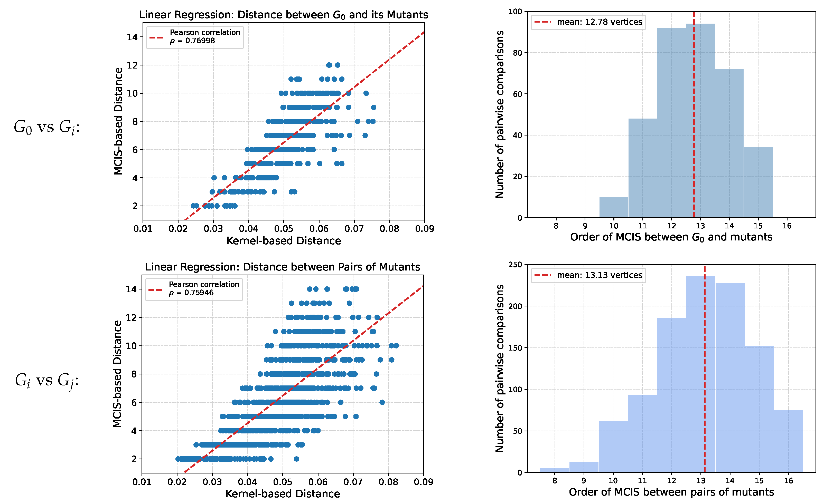
The mutation test graphs were used to investigate the correlation kernel-based and MCIS-based distance measures. Empirically, we find a good correlation indicating that the kernel-based distance, which can be evaluated much more efficiently, is a decent approximation for the purpose of constructing the guide tree (Figure A1).
In order to better characterize the set of test graphs, we show the distribution of MCIS-sizes for pairs of graphs. Typically, the MCIS covers more than half of both graphs, explaining why Iterative_Trimming is more efficient than VF2_step on this data set.
Figure A1.
Left: correlation between kernel distance and MCIS-based distance. Right: distribution of . The panels on the top compare the initial graph to its mutants. The panels below compare pairs of mutants over each of the 50 scenarios.
Figure A1.
Left: correlation between kernel distance and MCIS-based distance. Right: distribution of . The panels on the top compare the initial graph to its mutants. The panels below compare pairs of mutants over each of the 50 scenarios.

Appendix A.2. Insufficiency of the Standard Version of VF2
The standard version of VF2 uses an optimized routine for proposing candidate matches that might extend M (see Algorithm A1). Here, ⪯ denotes an arbitrary total order assigned by the VF2 to the vertices of , used to optimize the selection of these vertices.
| Algorithm A1: candidate_matches_original |
 |
The example in Figure A2 illustrates why the standard implementation cannot be used for an MCIS search. With the given total order ⪯, every branch of the search space produced by the VF2 will start with a pair of the form . Then, one branch will be associated to the match . Now, candidate_matches_original has to chose from pairs with as candidates. But, from these, the valid candidate will be given the condition on the minimum second entry. Since this pair does not satisfy the syntactic compatibility, see Section 3.3, this pair would not extend the match and the algorithm would backtrack. Thus, the MCIS enclosed in red dotted lines cannot be found by such implementation.
Figure A2.
Examples of a graph with given vertex order for which the standard choice of candidates, i.e., candidate_matches_original, does not result in the correct MCIS.
Figure A2.
Examples of a graph with given vertex order for which the standard choice of candidates, i.e., candidate_matches_original, does not result in the correct MCIS.

Similar examples show that other strategies such as “taking the feasible pair from the minimum” instead of the “minimum pair from the feasible” also fail for certain inputs. In general, the difference lies in that the VF2 assumes that there should be at least one match mapping every vertex in these graphs if they are indeed isomorphic, a condition that is not compatible with the MCIS search.
Appendix A.3. Additional Information on Ambiguous Edges
Figure A3 shows that the number of ambiguous edges increases substantially when a random guide tree is used instead of a similarity-based one.
Figure A3.
Distribution of ambiguous edges present in (a) alignments obtained when using the kernel-based guide trees, and (b) when using the random guide trees.
Figure A3.
Distribution of ambiguous edges present in (a) alignments obtained when using the kernel-based guide trees, and (b) when using the random guide trees.

Appendix A.4. Running Times
Figure A4 shows the distribution of the running times corresponding to the experiments and from Figure 7.
Figure A4.
Running times of both algorithms, (a) Iterative_Trimming and (b) VF2_Step, tested together with kernel-based guide trees but ignoring ambiguous edges.
Figure A4.
Running times of both algorithms, (a) Iterative_Trimming and (b) VF2_Step, tested together with kernel-based guide trees but ignoring ambiguous edges.

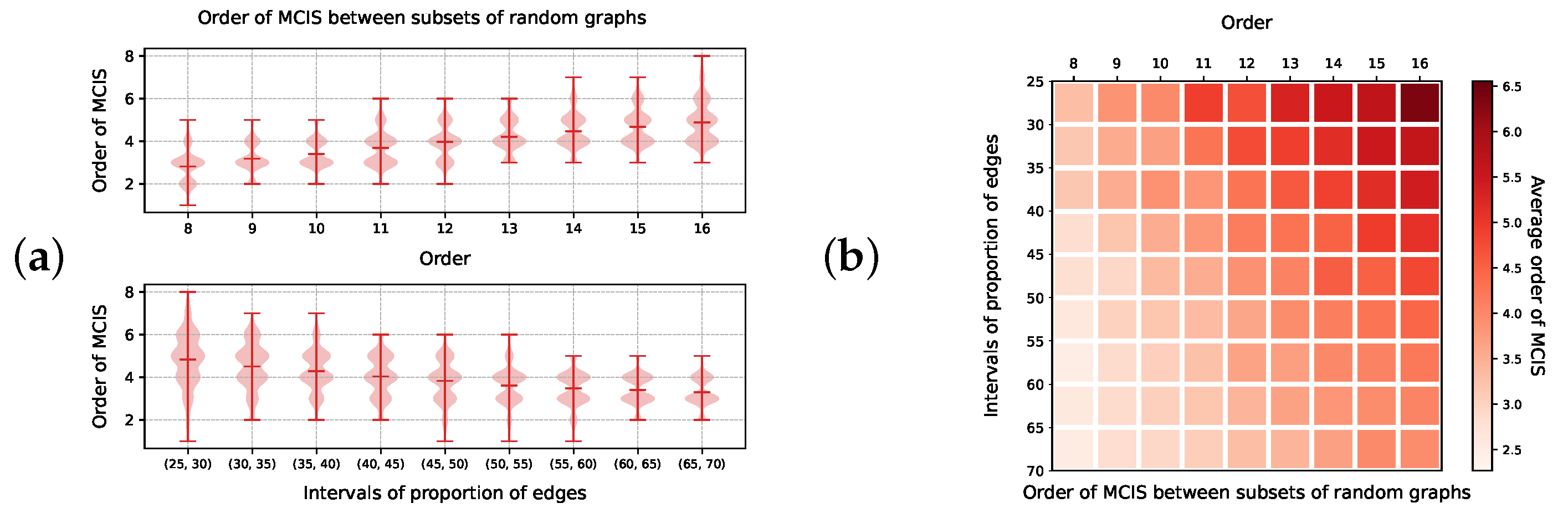
In order to further explore the behavior of different algorithmic variants, we produced another set of random graphs comprising connected graphs chosen uniformly, having between 8 and 16 vertices, and a number of edges in prescribed intervals. These graphs were assigned vertex and edge labels uniformly at random using five possible vertex and edge labels, respectively. For each parameter combination, a sample of 10 graphs was selected. Each subset with a given size and proportion of edges corresponds to a square in Figure A5b. We ran an MCIS search with our algorithms over these 10 graphs. The orders of the pairwise MCISs between these graphs are summarized in Figure A5a, with respect to the values of order and proportion of edges of the random graphs, and the average of the order of these MCIS’s is shown in Figure A5b over each pair of values.
Figure A5.
Order of MCIS between random graphs generated by pairs of order and proportion of edges, chosen uniformly and labeled uniformly at random. (a) Shows average variations against each variable, while (b) shows the variations against the combination of these parameters.
Figure A5.
Order of MCIS between random graphs generated by pairs of order and proportion of edges, chosen uniformly and labeled uniformly at random. (a) Shows average variations against each variable, while (b) shows the variations against the combination of these parameters.

In Figure A6, we show the running time taken for each algorithm to complete the MCIS-search in this data set. Specifically, Figure A6(a1,a2) show the running time of Iterative_Trimming, while Figure A6(b1,b2) show the one of VF2_step. The running time of the algorithms grows according to the order of the MCIS. However, VF2_step appears to grow inversely to the proportion of edges. Since the running time of the VF2_step must increase according to the number edges of a graph, this behavior can be better explained by the correlation between the running time taken by this routine with the order of the MCIS it has to uncover, shown in Figure A5b. This suggests that VF2_step is better suited for detecting MCISs that are comparatively smaller than the graphs containing them.
Figure A6.
Running time of MCIS-search over connected random graphs. Top corresponds to Iterative_Trimming and bottom to VF2_step. Again (a1,b1) show average variations against each variable, while (a2,b2) show the variations against pairs of order and proportion of edges.
Figure A6.
Running time of MCIS-search over connected random graphs. Top corresponds to Iterative_Trimming and bottom to VF2_step. Again (a1,b1) show average variations against each variable, while (a2,b2) show the variations against pairs of order and proportion of edges.

References
- Rosenberg, M.S. (Ed.) Sequence alignment: Concepts and history. In Sequence Alignment: Methods, Models, Concepts, and Strategies; University of California Press: Oakland, CA, USA, 2009; pp. 1–22. [Google Scholar] [CrossRef]
- Chatzou, M.; Magis, C.; Chang, J.M.; Kemena, C.; Bussotti, G.; Erb, I.; Notredame, C. Multiple sequence alignment modeling: Methods and applications. Brief. Bioinform. 2015, 17, 1009–1023. [Google Scholar] [CrossRef]
- Jiang, T.; Wang, L.; Zhang, K. Alignment of trees—An alternative to tree edit. Theor. Comput. Sci. 1995, 143, 137–148. [Google Scholar] [CrossRef]
- Höchsmann, M.; Voss, B.; Giegerich, R. Pure multiple RNA secondary structure alignments: A progressive profile approach. Trans. Comput. Biol. Bioinform. 2004, 1, 53–62. [Google Scholar] [CrossRef]
- Berkemer, S.; Höner zu Siederdissen, C.; Stadler, P.F. Compositional properties of alignments. Math. Comput. Sci. 2021, 15, 609–630. [Google Scholar] [CrossRef]
- Berg, J.; Lässig, M. Local graph alignment and motif search in biological networks. Proc. Natl. Acad. Sci. USA 2004, 101, 14689–14694. [Google Scholar] [CrossRef]
- Kuchaiev, O.; Milenković, T.; Memisević, V.; Hayes, W.; Pržulj, N. Topological network alignment uncovers biological function and phylogeny. J. R. Soc. Interface 2010, 7, 1341–1354. [Google Scholar] [CrossRef]
- Mernberger, M.; Klebe, G.; Hüllermeier, E. SEGA: Semiglobal graph alignment for structure-based protein comparison. IEEE/ACM Trans. Comput. Biol. Bioinform. 2011, 8, 1330–1343. [Google Scholar] [CrossRef] [PubMed]
- Weskamp, N.; Hüllermeier, E.; Kuhn, D.; Klebe, G. Multiple graph alignment for the structural analysis of protein active sites. IEEE/ACM Trans. Comput. Biol. Bioinform. 2007, 4, 310–320. [Google Scholar] [CrossRef] [PubMed]
- Singh, R.; Xu, J.X.; Berger, B. Global alignment of multiple protein interaction networks with application to functional orthology detection. Proc. Natl. Acad. Sci. USA 2008, 105, 12763–12768. [Google Scholar] [CrossRef]
- Zhang, S.; Tong, H. FINAL: Fast attributed network alignment. In Proceedings of the KDD ’16: Proceedings of the 22nd ACM SIGKDD International Conference on Knowledge Discovery and Data Mining, San Francisco, CA, USA, 13–17 August 2016; Krishnapuram, B., Shah, M., Smola, A., Aggarwal, C., Shen, D., Eds.; Association for Computing Machinery: New York, NY, USA, 2016; pp. 1345–1354. [Google Scholar] [CrossRef]
- Heimann, M.; Lee, W.; Pan, S.; Chen, K.Y.; Koutra, D. HashAlign: Hash-based alignment of multiple graphs. In Proceedings of the Advances in Knowledge Discovery and Data Mining, PAKDD 2018, Melbourne, VIC, Australia, 3–6 June 2018; Phung, D., Tseng, V., Webb, G., Ho, B., Ganji, M., Rashidi, L., Eds.; Lecture Notes in Computer Science; Springer: Cham, Switzerland, 2018; Volume 10939, pp. 726–739. [Google Scholar] [CrossRef]
- Bayati, M.; Gleich, D.F.; Saberi, A.; Wang, Y. Message-passing algorithms for sparse network alignment. ACM Trans. Knowl. Discov. Data 2013, 7, 3. [Google Scholar] [CrossRef]
- Tang, J.; Zhang, W.; Li, J.; Zhao, K.; Tsung, F.; Li, J. Robust attributed graph alignment via joint structure learning and optimal transport. In Proceedings of the IEEE 39th International Conference on Data Engineering (ICDE), Los Alamitos, CA, USA, 3–7 April 2023; pp. 1638–1651. [Google Scholar] [CrossRef]
- Malmi, E.; Chawla, S.; Gionis, A. Lagrangian relaxations for multiple network alignment. Data Min. Knowl. Discov. 2017, 31, 1331–1358. [Google Scholar] [CrossRef]
- Feng, D.F.; Doolittle, R.F. Progressive sequence alignment as a prerequisite to correct phylogenetic trees. J. Mol. Evol. 1987, 25, 351–360. [Google Scholar] [CrossRef]
- Wang, L.; Jiang, T. On the complexity of multiple sequence alignment. J. Comput. Biol. 1994, 1, 337–348. [Google Scholar] [CrossRef]
- Just, W. Computational complexity of multiple sequence alignment with SP-score. J. Comput. Biol. 2001, 8, 615–623. [Google Scholar] [CrossRef]
- Elias, I. Settling the intractability of multiple alignment. J. Comput. Biol. 2006, 13, 1323–1339. [Google Scholar] [CrossRef]
- Fober, T.; Mernberger, M.; Klebe, G.; Hüllermeier, E. Evolutionary construction of multiple graph alignments for the structural analysis of biomolecules. Bioinformatics 2009, 25, 2110–2117. [Google Scholar] [CrossRef]
- Ngoc, H.T.; Duc, D.D.; Xuan, H.H. A novel ant based algorithm for multiple graph alignment. In Proceedings of the International Conference on Advanced Technologies for Communications (ATC 2014), Hanoi, Vietnam, 15–17 October 2014; Heath, R.W., Quynh, N.X., Lap, L.H., Eds.; IEEE Press: Piscataway, NJ, USA, 2014; pp. 181–186. [Google Scholar] [CrossRef]
- Sokal, R.R.; Michener, C.D. A statistical method for evaluating systematic relationships. Univ. Kansas Sci. Bull. 1958, 38, 1409–1438. [Google Scholar]
- Cordella, L.P.; Foggia, P.; Sansone, C.; Vento, M. A (sub)graph isomorphism algorithm for matching large graphs. IEEE Trans. Pattern Anal. Mach. Intell. 2004, 26, 1367–1372. [Google Scholar] [CrossRef] [PubMed]
- Alpár Jüttner, A.; Madarasi, P. VF2++—An improved subgraph isomorphism algorithm. Discret. Appl. Math. 2018, 242, 69–81. [Google Scholar] [CrossRef]
- Touzet, H. Comparing similar ordered trees in linear-time. J. Discret. Algorithms 2007, 5, 696–705. [Google Scholar] [CrossRef]
- Stadler, P.F. Alignments of biomolecular contact maps. Interface Focus 2021, 11, 20200066. [Google Scholar] [CrossRef] [PubMed]
- Morgenstern, B.; Stoye, J.; Dress, A.W.M. Consistent Equivalence Relations: A Set-Theoretical Framework for Multiple Sequence Alignments; Technical Report; University of Bielefeld, FSPM: Bielefeld, Germany, 1999. [Google Scholar]
- Nelesen, S.; Liu, K.; Zhao, D.; Linder, C.R.; Warnow, T. The effect of the guide tree on multiple sequence alignments and subsequent phylogenetic analyses. In Pacific Sympomsium on Biocomputing PSB’08; Altman, R.B., Dunker, A.K., Hunter, L., Klein, T.E., Eds.; Stanford Univ.: Stanford, CA, USA, 2008; pp. 25–36. [Google Scholar] [CrossRef]
- Zhan, Q.; Ye, Y.; Lam, T.W.; Yiu, S.M.; Wang, Y.; Ting, H.F. Improving multiple sequence alignment by using better guide trees. BMC Bioinform. 2015, 16, S4. [Google Scholar] [CrossRef] [PubMed]
- Bunke, H. On a relation between graph edit distance and maximum common subgraph. Pattern Recognit. Lett. 1997, 18, 689–694. [Google Scholar] [CrossRef]
- Zeng, Z.; Tung, A.K.H.; Wang, J.; Feng, J.; Zhou, L. Comparing stars: On approximating graph edit distance. Proc. VLDB Endow. 2009, 2, 25–36. [Google Scholar] [CrossRef]
- Jia, L.; Gaüzère, B.; Honeine, P. Graph kernels based on linear patterns: Theoretical and experimental comparisons. Expert Syst. Appl. 2022, 189, 116095. [Google Scholar] [CrossRef]
- Schölkopf, B. The kernel trick for distances. In Proceedings of the NIPS’00: Proceedings of the 13th International Conference on Neural Information Processing Systems, Denver, CO, USA, 1 January 2000; Leen, T., Dietterich, T., Tresp, V., Eds.; MIT Press: Cambridge, MA, USA, 2000; pp. 283–289. [Google Scholar]
- Phillips, J.M.; Venkatasubramanian, S. A gentle introduction to the kernel distance. arXiv 2011, arXiv:1103.1625. [Google Scholar] [CrossRef]
- Kriege, N.M.; Johansson, F.D.; Morris, C. A survey on graph kernels. Appl. Netw. Sci. 2020, 5, 6. [Google Scholar] [CrossRef]
- Jia, L.; Gaüzère, B.; Honeine, P. Graphkit-learn: A python library for graph kernels based on linear patterns. Pattern Recognit. Lett. 2021, 143, 113–121. [Google Scholar] [CrossRef]
- Garey, M.R.; Johnson, D.S. Computers and Intractability. A Guide to the Theory of NP Completeness; Freeman: San Francisco, CA, USA, 1979. [Google Scholar]
- Kann, V. On the approximability of the maximum common subgraph problem. In Proceedings of the 9th Annual Symposium on Theoretical Aspects of Computer Science; Cachan, France, 13–15 February 1992; Finkel, A., Jantzen, M., Eds.; Lecture Notes in Computer Science; Springer: Berlin/Heidelberg, Germany, 1992; Volume 577, pp. 375–388. [Google Scholar] [CrossRef]
- Barrow, H.; Burstall, R. Subgraph isomorphism, matching relational structures and maximal cliques. Inf. Process. Lett. 1976, 4, 83–84. [Google Scholar] [CrossRef]
- McCreesh, C.; Prosser, P.; Trimble, J. A partitioning algorithm for maximum common subgraph problems. In Proceedings of the Twenty-Sixth International Joint Conference on Artificial Intelligence, IJCAI-17, Melbourne, Australia, 19–25 August 2017; Sierra, C., Ed.; AAAI Press: Palo Alto, CA, USA, 2017; pp. 712–719. [Google Scholar] [CrossRef]
- Hoffmann, R.; McCreesh, C.; Reilly, C. Between subgraph isomorphism and maximum common subgraph. In Proceedings of the Thirty-First AAAI Conference on Artificial Intelligence, San Francisco, CA, USA, 4–9 February 2017; Markovitch, S., Singh, S., Eds.; AAAI Press: Palo Alto, CA, USA, 2017; Volume 1, pp. 3907–3914. [Google Scholar] [CrossRef]
- Liu, Y.; Zhao, J.; Li, C.M.; Jiang, H.; He, K. Hybrid learning with new value function for the maximum common induced subgraph problem. In Proceedings of the Thirty-Seventh AAAI Conference on Artificial Intelligence (AAAI-37), Washington, DC, USA, 7–14 February 2023; Williams, B., Chen, Y., Neville, J., Eds.; AAAI Press: Palo Alto, CA, USA, 2023; Volume 4, pp. 4044–4051. [Google Scholar]
- Berezikov, E.; Guryev, V.; Plasterk, R.H.A.; Edwin, C. CONREAL: Conserved regulatory elements anchored alignment algorithm for identification of transcription factor binding sites by phylogenetic footprinting. Genome Res. 2004, 14, 170–178. [Google Scholar] [CrossRef]
- Morgenstern, B.; Prohaska, S.J.; Pohler, D.; Stadler, P.F. Multiple sequence alignment with user-defined anchor points. Algorithms Mol. Biol. 2006, 1, 6. [Google Scholar] [CrossRef]
- Brun, L.; Gaüzère, B.; Fourey, S. Relationships between Graph Edit Distance and Maximal Common Unlabeled Subgraph; Technical Report hal-00714879; HAL: Bangalore, India, 2012. [Google Scholar]
- Hagberg, A.A.; Schult, D.A.; Swart, P.J. Exploring network structure, dynamics, and function using NetworkX. In Proceedings of the 7th Python in Science Conference, Pasadena, CA, USA, 19–24 August 2008; Varoquaux, G., Vaught, T., Millman, J., Eds.; 2008; pp. 11–15. [Google Scholar]
- González-Laffitte, M.E.; Stadler, P.F. Github Repository of the Progressive Graph Alignment Software ProGrAlign. 2024. Available online: https://github.com/MarcosLaffitte/Progralign (accessed on 23 February 2024).
- Documentation on the Pickle Python Package. Available online: https://docs.python.org/3/library/pickle.html (accessed on 1 March 2024).
- Hunter, J.D. Matplotlib: A 2D graphics environment. Comput. Sci. Eng. 2007, 9, 90–95. [Google Scholar] [CrossRef]
- Schneider, T.D. Consensus sequence zen. Appl. Bioinform. 2002, 1, 111–119. [Google Scholar]
- Hagiwara, K.; Edmonson, M.N.; Wheeler, D.A.; Zhang, J. indelPost: Harmonizing ambiguities in simple and complex indel alignments. Bioinformatics 2022, 38, 549–551. [Google Scholar] [CrossRef] [PubMed]
- Giegerich, R. Explaining and controlling ambiguity in dynamic programming. In Proceedings of the Combinatorial Pattern Matching. CPM’00, Montreal, QC, Canada, 21–23 June 2000; Giancarlo, R., Sankoff, D., Eds.; Lecture Notes in Computer Science; Springer: Berlin/Heidelberg, Germany, 2000; Volume 1848. [Google Scholar] [CrossRef]
- Wallace, I.M.; Orla, O.; Higgins, D.G. Evaluation of iterative alignment algorithms for multiple alignment. Bioinformatics 2005, 21, 1408–1414. [Google Scholar] [CrossRef] [PubMed]
- Sze, S.H.; Lu, Y.; Wang, Q.W. A polynomial time solvable formulation of multiple sequence alignment. J. Comput. Biol. 2006, 13, 309–319. [Google Scholar] [CrossRef]
Figure 2.
Progressive graph alignment of three graphs (bottom) along a guide tree (fat red edges). The matching of vertices is shown by vertical lines. Two of the ambiguous edges in the pairwise alignment, which are inserted due to the matches with the third graph, are shown in green.
Figure 2.
Progressive graph alignment of three graphs (bottom) along a guide tree (fat red edges). The matching of vertices is shown by vertical lines. Two of the ambiguous edges in the pairwise alignment, which are inserted due to the matches with the third graph, are shown in green.

Figure 3.
Visualization of a graph alignment of three input graphs. Top: matrix representation highlighting presence/absence of input graphs in the alignment columns (rows). Vertex-labels may be represented by colors. Middle: each of the three input graphs is shown embedded in the alignment graph. Matched vertices are shown in corresponding positions and with corresponding colors. Bottom: graph of the multiple graph alignment.

Figure 4.
Example of the 3D visualization of an alignment by stacking planar embeddings of the graphs. Vertex colors again encode the arbitrary vertex-labels that can be assigned to the input graphs. The bottom graph with grey vertices is the embedding of the final alignment, which, in principle, may be computed with or without the preservation of vertex-labels and/or edge-weights and edge-labels.

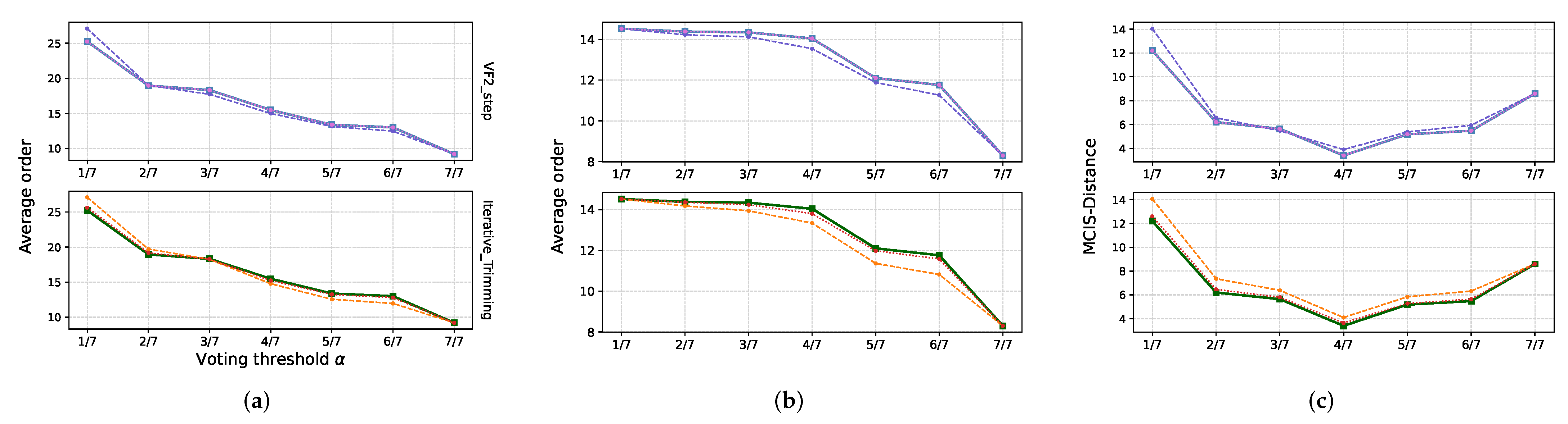
Figure 5.
Consensus graphs as function of the voting threshold . (a) The size of the consensus, as expected, decreases monotonously with increasing fraction of non-gaps in the retained alignment columns. (b) Correspondingly, the fraction of the vertices of the input graphs that are retained in the consensus decreases. (c) The distance between the reference graph and the alignment of its noisy offspring through , however, reaches a minimum when only the columns that contain less then 50% gaps are used to form the consensus. In each panel, we compare guide trees computed with kernel-based similarity (full lines), random guide trees without considering ambiguous edges (dashed lines), and random guide trees taking ambiguous edges into account (dotted lines). The latter are nearly indistinguishable form the kernel-based guide trees. Here line colors are a visual aid to distiguish the methodologies and their variations outlined before.

Figure 6.
Correlation of the number of ambiguous edges with the number of gaps. The values here correspond to the 400 alignments resulting from running the 8 experiments, described in Figure 7, over our set of 50 scenarios.
Figure 6.
Correlation of the number of ambiguous edges with the number of gaps. The values here correspond to the 400 alignments resulting from running the 8 experiments, described in Figure 7, over our set of 50 scenarios.

Figure 7.
Comparison of running times [s] of the eight experiments carried each over the 50 scenarios: T and S refer to the use of Iterative_Trimming and VF2_step, respectively. Kernel-based (k) or random (r) guide trees show a moderate but systematic advantage of a kernel-based similarity. The exclusion (◯) or inclusion (■) of ambiguous edges is also compared.

Disclaimer/Publisher’s Note: The statements, opinions and data contained in all publications are solely those of the individual author(s) and contributor(s) and not of MDPI and/or the editor(s). MDPI and/or the editor(s) disclaim responsibility for any injury to people or property resulting from any ideas, methods, instructions or products referred to in the content. |
© 2024 by the authors. Licensee MDPI, Basel, Switzerland. This article is an open access article distributed under the terms and conditions of the Creative Commons Attribution (CC BY) license (https://creativecommons.org/licenses/by/4.0/).
Share and Cite
MDPI and ACS Style
González Laffitte, M.E.; Stadler, P.F. Progressive Multiple Alignment of Graphs. Algorithms 2024, 17, 116. https://doi.org/10.3390/a17030116
AMA Style
González Laffitte ME, Stadler PF. Progressive Multiple Alignment of Graphs. Algorithms. 2024; 17(3):116. https://doi.org/10.3390/a17030116
Chicago/Turabian StyleGonzález Laffitte, Marcos E., and Peter F. Stadler. 2024. "Progressive Multiple Alignment of Graphs" Algorithms 17, no. 3: 116. https://doi.org/10.3390/a17030116
Note that from the first issue of 2016, this journal uses article numbers instead of page numbers. See further details here.