Semi-empirical Algorithm for the Retrieval of Ecology-Relevant Water Constituents in Various Aquatic Environments

Abstract

An advanced operational semi-empirical algorithm for processing satellite remote sensing data in the visible region is described. Based on the Levenberg-Marquardt multivariate optimization procedure, the algorithm is developed for retrieving major water colour producing agents: chlorophyll-a, suspended minerals and dissolved organics. Two assurance units incorporated by the algorithm are intended to flag pixels with inaccurate atmospheric correction and specific hydro-optical properties not covered by the applied hydro-optical model. The hydro-optical model is a set of spectral cross-sections of absorption and backscattering of the colour producing agents. The combination of the optimization procedure and a replaceable hydro-optical model makes the developed algorithm not specific to a particular satellite sensor or a water body. The algorithm performance efficiency is amply illustrated for SeaWiFS, MODIS and MERIS images over a variety of water bodies.

1. Introduction

Throughout the recent decades, satellite remote sensing of the world oceans became increasingly important in light of both the problem of global climate change and frequent deterioration of the aquatic ecology status, the latter being driven by ever increasing needs of growing populations for drinking water as well as for fish and other sea food.

Satellite-based sensors operating in the visible are most suited for this mission as only the visible radiation penetrates appreciably into the water column and its backscattered component carries the desired information about the quality of water bodies under surveillance.

Several satellite sensors, such as Sea-viewing Wide Field-of-view Sensor (SeaWiFS), Moderate Resolution Imaging Spectroradiometer (MODIS), and Medium Resolution Imaging Spectrometer (MERIS), operate in the visible and near infrared and provide global coverage. The main challenge resides in the retrieval of exact information about water quality parameters from the collected images.

The approaches to the retrieval of water quality parameters from spaceborne data depend on the optical complexity of the target water body. According to Morel and Prieur [1], all natural waters are partitioned into case 1 and case 2 waters. In case 1 waters, variations of the aquatic medium optical properties (and hence water colour) are predominantly controlled by phytoplankton and co-varying products of their life cycle. Colour variations in case 2 waters are controlled not only by phytoplankton and their accompanying retinue, but also by other substances, notably terrigenous suspended minerals (sm) and allochthonous dissolved organic matter (doc) that vary independently of phytoplankton.

In case 1 waters (mostly open ocean waters), algorithms for the retrieval of the desired water quality parameter, e.g. the phytoplankton abundance, are rather unsophisticated. For instance, the case 1 water OC4 algorithm currently used by the National Aeronautics and Space Administration (NASA) [2,3] is based on a relationship between the concentration of phytoplankton chlorophyll, chl (a proxy of the phytoplankton abundance) and the emerging radiance at two or more wavelengths normalized to the incident irradiance at the same wavelengths.

In case 2 waters, this approach is untenable as the radiation emerging from beneath the water surface is affected at any wavelength not solely by phytoplankton, but other substances as well. Therefore, in order to retrieve one component, e.g. chl it is necessary to infer simultaneously the content of other water constituents affecting the water colour, so called colour producing agents (CPAs), first and foremost, sm and doc. Together with chl, sm, doc and such substances as total organic carbon (toc) and total suspended sediments (tss) are traditionally categorized as water quality parameters (WQP).

One of the possible solutions of the problem of WQP retrieval from satellite images collected over case 2 waters is the application of an algorithm based upon the Levenberg-Marquardt (LM) multivariate optimization procedure [4,5]. The main advantage of the LM algorithm comparing to such algorithms as band ratio algorithms or neural networks is higher accuracy in inverse problem solution [6,7,8]. As our experience shows other multivariate optimization techniques (as genetic algorithms) prove to be at least twice more time consuming.

In the “Methods” section we begin with a concise description of the basic principles of the LM technique, assessment of the algorithm efficiency. In the same section we also focus on the development and characteristics of hydro-optical models. The next section, “The algorithm applications”, is devoted to the assessment of the developed algorithm efficiency in some case studies. In “Discussions” we describe possible sources of errors and the favourable conditions for the algorithm application.

2. Methods

In our study we operate with the subsurface spectral remote sensing reflectance [noted in the literature as R_rsw(λ, C, a, b_b)], which is the upwelling spectral radiance just beneath the water-air interface, L(-0, λ) normalized to the downwelling spectral irradiance, E(-0, λ) at the same level [9]). Let S be the spectrum of R_rsw which is calculated from remote sensing data or from in situ optical observations (measured reflectance).

Subsurface spectral remote sensing reflectance depends on the vector of all the major CPA concentrations and on their inherent optical properties (IOPs). These properties are the specific (normalized to the respective unit concentration) spectral absorption a* and backscattering, b_b* coefficients of the coexisting water constituents (e.g. a*_chl, a*_sm, a*_doc, b_b*_chl, b_b*_sm ).

Let T be the spectrum of R_rsw calculated using the empirical equation derived from numerical Monte Carlo simulations by Jerome [9]:

T = – 0.00036 + 0.110(b_b/a) – 0.0447(b_b/a)²

(1)

where a and b_b are the water column bulk absorption and backscattering coefficients correspondingly.

Being additive by nature, the coefficients a and b_b are sums of respective contributions (C_ia*_i, C_jb_b*_j) from the major CPAs:

$$a=a_w+{\displaystyle \sum _i{C}_i}{a}_i^{*},$$

(2)

$$b_b=b_{bw}+{\displaystyle \sum _j{C}_j}{b_b}_j^{*},$$

(3)

where i and j are the indices of the absorbing and scattering components (e.g. chl, sm or doc). Using equations (1-3) we can calculate the reflectance spectrum T (reconstructed reflectance) for any vector of CPA concentrations if the set of respective IOPs (i.e. hydro-optical model) is given.

The relationship (1) was developed for case 2 waters [10], similar approaches e.g. by H. Gordon are designed for case 1 waters.

2.1. Multivariate Optimization Procedure

For a vector of concentrations C and a given hydro-optical model the residual between measured and reconstructed reflectance at j-th wavelength can be computed as follows:

g_j = (S_j – T_j) / T_j

(4)

The multidimensional least-square solution using all wavelengths is found by minimizing the sum of squared residuals by simultaneous variation of concentrations in the vector C:

$$f(\mathit{C})={\displaystyle \sum _j{g}_j^2}(\mathit{C})$$

(5)

The absolute minimum of f (C) can be found with the Levenberg-Marquardt finite difference algorithm [4,5], which assures a rapid convergence of the iterative procedure. The following iterative expression is used to this goal:

$${\mathit{C}}_{k+1}={\mathit{C}}_k+{\zeta }_k{(F_k^t{F}_k+{\mu }_k{D}_k)}^{-1}{F}_k^t\left(1-\frac{T({\mathit{C}}_k)}{\left\{S_k\right\}}\right)$$

(6)

where $k$ = iteration step, $D_k=diag(F_k^t{F}_k)=$ diagonal matrix consisting of the elements $F_k^t{F}_k$, with $F(\mathit{C})=\left|\frac{\partial T_j}{\partial {\mathit{C}}_j}\right|=$ matrix composed of n x m elements (n = number of wavelengths, at which the measurements of S_j have been conducted, m = dimension of the concentration vector C), $F^t(\mathit{C})$ = transposed matrix, ${\mu }_k$ = direction of minimization, ${\zeta }_k$ = length of the minimization step. The criterion for the termination of the iterative procedure is f (C) ≤ 10^-5.

The actual length, ${\zeta }_k$ can be chosen easily and effectively through applying the method of reduction, which consists in the following: at a certain iteration step $k$ a deliberately high value of ${\zeta }_k$ is chosen (e.g. 50). From eq. 3 a new concentration vector ${\mathit{C}}_{k+1}$ is determined, for which the inequality $f({\mathit{C}}_{k+1})<f({\mathit{C}}_k)$ is tested. If it is not satisfied, ${\zeta }_k$ is reduced by a factor of two, and a new round of search is initiated. This iterative procedure is continued until the above inequality is satisfied, i.e. until the newly determined concentration vector proves to be closer to the minimum of the function of residuals f (C) as compared to the concentration vector established in the previous iteration step.

In the course of the iterative descent to the global minimum of the function of residuals, the above procedure could end up in a local minimum. If the determined concentration vector, ${\mathit{C}}_k$ happens to be on the downhill and the length of the iteration step $\zeta$ is sufficiently high, then the next concentration vector ${\mathit{C}}_{k+1}$ might occur on the downhill in the direction to a deeper minimum. In this case the process of search will move to a new point provided the inequality $f({\mathit{C}}_{k+1})<f({\mathit{C}}_k)$ is satisfied. Thus, such a search with a variable length $\zeta$ can, under favourable conditions, evade a local minor minimum and end either in a deeper or even in the global minimum.

However, equally possible is the situation that the concentration vector ${\mathit{C}}_{k+1}$ is on the uphill side of a certain local minimum of f (C). In this case the search ends in this local minimum, which corresponds to an inadequate solution of the inverse problem. Naturally, the probability for the latter option increases with measurement errors.

To avoid the above difficulty, it is advisable to initiate the iteration procedure for an array of initial guess values, C₀. Afterwards the deepest minimum of f (C) is selected. The number N of the initial vectors C₀ should not be excessively high because the computation time for the inverse problem solution increases proportionally with N.

But the use of an array of initial vectors C₀ does not guarantee that the iterative procedure will be converging or the eventually established concentration vector C be realistic. To overcome this problem, some a priori limits can be imposed upon each of CPA concentrations, C_i:

$$C_{i\min }\le C_i\le C_{i\max }$$

(7)

where i is the ith constituent of the aquatic medium.

2.2. Assessment of Robustness of the LM Procedures against Simulated Measurement Errors

The LM procedure in the Matlab environment has been realized using the recipes given by Press [11]. The code for the L-M procedure used in the present study was developed by one of us (A. Korosov) using the C++ language. Calculations of the resultant bulk absorption and backscattering coefficients for the simulated aquatic medium were performed by using the hydro-optical model suggested by Kondratyev [12,10]. The model is a collection of tabulated spectral values of a* and b_b* for the major CPAs, i.e. chl, sm and doc within the spectral region 400-700 nm, as obtained for case 2 waters with the trophic status varying from oligotrophic to eutrophic.

In order to test the algorithm performance, the following numerical experiment was carried out. 1000 concentration vectors (C = {C_chl, C_sm, C_doc}) were randomly selected in rather wide ranges (0-70 μg/L; 0-30 mg/L and 0-30 mgC/L for chl, sm and doc, respectively). One thousand spectra of T were generated from concentration vectors using equations 1, 2 and 3. Another 13,000 spectra of S were simulated by contaminating the calculated T with ‘noise’ for the following options:

• four levels of noise in input data: 0, 5, 10 and 15%;
• two types of noise distribution: uniform and normal;
• two types of λ-dependency: noise is independent and dependent on λ (the spectral dependence was assumed to be linearly decreasing with λ) [13,14].

Our comparison of simulated and retrieved results showed a very high retrieval accuracy for the case with a zero input noise (correlation, r equals 0.999 for all three parameters, root mean square error, RMSE equals 1.8 μg/L for chl, 1.0 mg/L for sm and 1.5 mgC/L for doc). Moreover, our simulations indicate that the L-M procedure remains stable for measurement errors up to 15 %. It was also found that the error level and its distribution as well as its dependence on λ strongly influence the attainable retrieval accuracy. The latter is also a function of the CPA concentration vector per se.

For oceanographic and limnological research we assume that, at least, for case 2 waters, the chl retrieval errors specified in Table 1 for a number of concentration ranges are admissible [15]. The simulations indicate that these accuracy requirements can only be fulfilled for specific hydro-optical conditions, i.e. the concentrations of chl, sm and doc have to fall into specific concentration ranges (Table 2).

Table 1. Acceptable accuracy of chl retrieval for different chl concentration ranges

chl range, μg/L	0 - 5	5 - 10	10 - 20	20 - 30
admissible error, %	50	40	30	20

Table 1. Acceptable accuracy of chl retrieval for different chl concentration ranges

chl range, μg/L	0 - 5	5 - 10	10 - 20	20 - 30
admissible error, %	50	40	30	20

Our simulations also indicate (Table 2) that the sm and doc concentration ranges (within which the LM procedure yields chl retrieval results with the permissible error as in table 1) shrink with increasing measurement error. The most stringent limitations arise in the case of normally distributed and λ-dependent measurement errors.

Under favourable conditions (e.g. when doc and sm concentrations are in the range 0–2 mgC/L and 0–0.5 mg/L respectively, and the noise is λ-independent) chl concentrations can be retrieved with acceptable accuracy in the entire range 0–30 μg/L (the corresponding cell is marked with asterisk in Table 2). In turbid waters (C_sm varies within 5–10 mg/L, C_doc – within 5–10 mgC/L) and with λ-dependent noise (the corresponding cell is marked with double asterisk) chlorophyll can be retrieved accurately only in the range 0–5 μg/L.

However, the dependence of measured errors on λ is inherent in satellite images subjected to the applied atmospheric correction procedure, as its base is the extrapolation of the aerosol path radiance determined in the near infrared to the blue spectral region [13,14]. It can, nevertheless, be expected that atmospheric correction approaches based on other concepts, such as the inversion method [16], or the methods of statistical regularization [17], multivariate optimization, neural networks, etc. would result in λ-independent errors. This would broaden considerably the range of hydro-optical conditions, in which the desired accuracy of chl retrieval can be reached.

Table 2. Ranges of C_chl, within which the chl retrieval accuracy specified in Table 1 is attainable given various options of doc and sm abundance in water and the spectral behavior of noise. Single- and double-asterisked entries exemplify the water composition situations that are, respectively, favourable and unfavourable for remote sensing of chl.

Error type	Cdoc, mgC/L	Csm, mg/L
		0-0.5	0.5-1	1-5	5-10	10-20
λ-independent	0-2	0–30*	0–30	0–30	0–30	0–30
	2-5	0-30	5-30	0-30	0-30	0-30
	5-10	0-30	0-30	0-30	0-30	0-30
	10-20	0-30	5-30	5-30	0-30	5-30
λ-dependent	0-2	0-5	0-5	0-5	0-5	0-5
	2-5	-	-	0-5	0-5	0-5
	5-10	-	-	-	0-5**	0-5
	10-20	-	-	-	-	-

Table 2. Ranges of C_chl, within which the chl retrieval accuracy specified in Table 1 is attainable given various options of doc and sm abundance in water and the spectral behavior of noise. Single- and double-asterisked entries exemplify the water composition situations that are, respectively, favourable and unfavourable for remote sensing of chl.

Error type	Cdoc, mgC/L	Csm, mg/L
		0-0.5	0.5-1	1-5	5-10	10-20
λ-independent	0-2	0–30*	0–30	0–30	0–30	0–30
	2-5	0-30	5-30	0-30	0-30	0-30
	5-10	0-30	0-30	0-30	0-30	0-30
	10-20	0-30	5-30	5-30	0-30	5-30
λ-dependent	0-2	0-5	0-5	0-5	0-5	0-5
	2-5	-	-	0-5	0-5	0-5
	5-10	-	-	-	0-5**	0-5
	10-20	-	-	-	-	-

Note that the boxes in Table 2 with no entries (-) imply that the LM procedure will not ensure the accuracy of chl retrieval with the admissible error.

2.3. LM-Based Hydro-Optical Retrieval Algorithm

The principal flow-diagram of our LM-based algorithm is given in Figure 1. An atmospherically corrected satellite image from SeaWiFS or MODIS is used to calculate the corresponding subsurface remote sensing reflectance spectrum S(λ)for each pixel [10] making use of the normalized upwelling radiance [L_w(λ)]_N. Images from these sensors are downloaded from the NASA OCEANCOLOR web site [18] in Level-2 format.

MERIS image processing includes calculation of S(λ) from the provided values of remote sensing reflectance above water R_rs(+0, λ). These images are downloaded either from the ESA rolling archive [19] or from the MERCI catalogue [20] in Level-2 format.

In the next step, the spectral curvature of S(λ) is automatically analysed to eliminate pixels with a) negative values of S at short wavelengths (400-450 nm) due to overestimation of the path radiance, and b) enhanced values of S in one or two first sensor channels followed by a dip in either the second or third channel due to underestimation of the path radiance.

Further, the algorithm calculates the gradient of the processed S spectrum starting from the first channel (i.e. the shortest wavelength) and moving to the red portion of the spectrum (towards the longest wavelength in the visible). The pixel is preserved only if the corresponding spectrum exhibits a stable positive gradient at λ < ~ 560 nm (it is allowed to be just non-negative at λ ≤ 450nm), followed by a negative gradient for λ > ~ 560 nm. The pixel is flagged, if it does not satisfy this requirement. However, this mask does not discard pixels with the S spectra characteristic of clear waters, should they be present in the image. Identification of clear and turbid waters is performed through jointly analyzing both the envelope of S spectra and their mean spectral value. The latter is known [21] to be distinctly different for clear and turbid waters, and a corresponding threshold is applied to this end.

Figure 1. A flow-diagram of the developed algorithm performance.

Figure 1. A flow-diagram of the developed algorithm performance.

For the remaining pixels the derived S is sent to the LM unit. The algorithm code is designed in such a way that there is a possibility of choosing an appropriate hydro-optical model from the embedded collection of hydro-optical models. The LM unit yields simultaneously the concentrations of chl, sm and doc.

The algorithm has a quality assessment/assurance unit whose function is to detect pixels corresponding to water areas whose hydro-optical properties significantly differ from those covered by the chosen hydro-optical model. This is done through calculating T using the retrieved concentration vector and the adopted hydro-optical model and the parametric relationship T = f(a, b_b). The reconstructed spectrum T is then compared with the initial spectrum S derived from the acquired satellite image. The pixel becomes flagged if the difference (S – T)² surpasses a certain threshold (10^-5 sr^-1) established experimentally.

2.4. Development of hydro-optical models

As seen in Section 2.1., the solution of the inverse problem resides in determining the concentration vector C given the spectral values of CPA specific coefficients of absorption and backscattering, i.e. a hydro-optical model. Such a model can be obtained through different ways. The following sections describe our approaches with regard to the case studies discussed in this paper.

2.4.1. Lake Ladoga hydro-optical model

In the second part of the 1980s, during the summer-time of three consecutive years, a large-scale ship campaign was conducted across the entire Lake Ladoga. In the course of this campaign, concurrently measured were spectral subsurface upwelling, E_u(-0,λ) and downwelling, E_d(-0,λ) irradiances to obtain spectral volume reflectance, R(λ) = E_u(-0,λ) / E_d(-0,λ), which is related to bulk coefficients of absorption, a(λ) and backscattering b_b*(λ) [21] and the concentrations of chl, sm and doc. These data were employed for the development of a hydro-optical model of Lake Ladoga. To do this, the LM procedure (section II) was exploited, this time for determining specific spectral coefficients of absorption, a*_i(λ) and backscattering b_b*_j(λ) (Fig. 2) of the water constituents addressed in this study (for details see [12]).

It is important to underline that in the hydro-optical model of Lake Ladoga, a*_doc is calculated through the normalization to the total doc concentration, i.e. not solely to the weight of the coloured fraction (called yellow substance or gelbstoff) - cdom. This has been done in order to facilitate the use of satellite data for validation of ecological models, which generally do not differentiate between sunlight-absorbing and non-absorbing doc fractions. Such an approach opens door to the assimilation of satellite retrievals by aquatic ecological models.

Figure 2. Spectra of specific absorption (upper row of plates) and specific backscattering (second row of plates) for three hydro-optical models: 1 - Lake Ladoga; 2 – North Sea; 3 – Lake Erie. For chlorophyll (left column), the absorption and backscattering values are in m²/mg, for suspended minerals (central column), – in m²/g and for DOC (right column), – in m²/gC. Wavelengths on the X-axe are in nm.

Figure 2. Spectra of specific absorption (upper row of plates) and specific backscattering (second row of plates) for three hydro-optical models: 1 - Lake Ladoga; 2 – North Sea; 3 – Lake Erie. For chlorophyll (left column), the absorption and backscattering values are in m²/mg, for suspended minerals (central column), – in m²/g and for DOC (right column), – in m²/gC. Wavelengths on the X-axe are in nm.

The efficiency of the developed algorithm performance was tested based on a fraction of the shipborne measurements that were not used for the hydro-optical model development. Table 3 lists WQP concentrations measured in situ and retrieved from spectral volume reflectance concurrently measured at the same locations.

Table 3. Comparison of the chl, sm and doc concentrations measured in situ and retrieved from shipborne optical measurements in Lake Ladoga

Measured concentrations			Retrieved concentrations
Cchl, μg/L	Сsm, mg/L	Сdoc, mgC/L	Cchl, μg/L	Сsm, mg/L	Сdoc, mgC/L
0.5	0.2	8	0.3	0.2	7
6.6	1.0	9	5.5	1.1	10
1.0	0.4	9	1.0	0.4	8
0.6	0.3	9	0.8	0.2	7
0.5	0.3	8	0.8	0.2	7
1.0	0.2	8	1	0.05	9
3.9	1.0	8	4	1.0	8
7.1	0.8	8	9	1.0	7
0.9	0.3	8	1	0.3	6
2.1	0.3	8	1.5	0.3	7
Correlation (r)			0.96	0.98	0.43
Root mean square error (RMSE)			0.73	0.096	1.2

Table 3. Comparison of the chl, sm and doc concentrations measured in situ and retrieved from shipborne optical measurements in Lake Ladoga

Measured concentrations			Retrieved concentrations
Cchl, μg/L	Сsm, mg/L	Сdoc, mgC/L	Cchl, μg/L	Сsm, mg/L	Сdoc, mgC/L
0.5	0.2	8	0.3	0.2	7
6.6	1.0	9	5.5	1.1	10
1.0	0.4	9	1.0	0.4	8
0.6	0.3	9	0.8	0.2	7
0.5	0.3	8	0.8	0.2	7
1.0	0.2	8	1	0.05	9
3.9	1.0	8	4	1.0	8
7.1	0.8	8	9	1.0	7
0.9	0.3	8	1	0.3	6
2.1	0.3	8	1.5	0.3	7
Correlation (r)			0.96	0.98	0.43
Root mean square error (RMSE)			0.73	0.096	1.2

The developed algorithm restores the desired concentrations with an average error in the range about 6–12%. The attained accuracy is high enough, and indicates the intrinsic capacity of the developed LM algorithm to accurately retrieve the desired concentrations inasmuch as the adopted verification procedure excludes the intervening factor of imprecise atmospheric correction.

2.4.2. The North Sea hydro-optical model

For the North Sea the intrinsic hydro-optical model (Figure 2) has been obtained under the ESA GMES MarCoast shipborne campaign encompassing cruises in the coastal areas of southern Norway. Water samples were collected to determine the concentration vector constituted by chl, total suspended matter (tsm), and absorption at 443 nm by yellow substance plus non-pigmented/detrital particulate matter. Concurrently with water sampling, surface reflectance, ρ_w(λ) was measured at six wavelengths (412, 443, 490, 510, 555, and 665 nm), where ρ_w(λ) is related to R_rsw via the coefficient of proportionality k = 0.587 sr^-1. A detailed description of this hydro-optical model is given elsewhere [22]. The water sampling and laboratory analyses were conducted in accordance with methods described in [23].

2.4.3. Lake Erie hydro-optical model

A rather extensive field campaign (over 60 stations) was being conducted by the Michigan State University (MTU) across Lake Erie in 2005 during June – September. The in situ measurements encompassed spectrometric measurements to retrieve subsurface remote sensing reflectance, R_rsw(λ) at 6 MODIS wavelengths in the visible (412, 443, 488, 531, 551, 667 nm) as well as the concentrations of chl, sm and doc.

The Lake Ontario hydro-optical model [21] was selected as a starting option for elaborating the Lake Erie hydro-optical model (Fig. 2). An iterative algorithm was used to find the desired five variables (i.e. a^*_chl, b_b^*_chl, a^*_sm, b_b^*_sm, a^*_doc:).

In each iteration step:

• the a^*_chl, b_b^*_chl, a^*_sm, b_b^*_sm, a^*_doc cross-sections for Lake Ontario are shifted up or down using the following equation (example for a*_chl ):

  a*_{chl i} = a*_{chl 0} + O_chl

  (8)

  where a_{chl i} is the value of a*_chl in the ith iteration step, a*_{chl 0} is the value of a*_chl for Lake Ontario, O_chl is the random offset for a*_chl;
• the shifted hydro-optical model is further used for the retrieval of CPA concentrations from the R_rsw(λ) values measured in situ employing our LM- based algorithm;
• the difference between the retrieved and measured CPA concentration vector C is then calculated. In performing this step, only the difference between the concentrations of chl and sm was tested;
• the obtained difference is further used for the selection of the best vector O. This step yields five offsets (O_achl, O_bbchl, O_asm, O_bbsm, O_docl,) that are further used for calculating a rough hydro-optical model for Lake Erie.

Thus, due to application of the above procedure, the cross-sections of the established rough model only differ from the Ontario cross-sections by offsets O. However, in reality, the spectral distributions of the desired CPA cross-sections can also differ from the “benchmark” model in terms of their spectral envelope. In order to accommodate this option and reveal possible spectral deviations of the sought for hydro-optical model from the “benchmark” model, applied were both the LM optimization technique and the Genetic algorithm [11] to find the best set of $a^{*}$ and $b_b^{*}$ in each channel. The results (i.e. desired spectral specific absorption and backscattering coefficients) proved to be very similar.

The LM optimization was run six times (for six channels), and it was found that a* and b_b* values in different MODIS channels were independent. In each step of the LM optimization:

• R_rsw values in a certain channel were calculated using the established five spectral values of $a^{*}$ and $b_b^{*}$ (a^*_chl, b_b^*_chl, a^*_sm, b_b^*_sm, a^*_doc) and the CPA concentrations. All three concentrations measured in situ were used to calculate R_rsw(λ);
• the calculated spectral values of R_rsw were further compared with the measured ones and the respective cost function f was determined;
• the Jacobian of f was calculated;
• each optimization iteration was run using the estimated cost function and calculated Jacobian;
• vectors a* and b_b*(i.e. a^*_chl, b_b^*_chl, a^*_sm, b_b^*_sm, a^*_doc) were modified according to the yield of the previous iteration step;

In each iteration step, each of the above 5 variables (i.e. the above specific absorption and backscattering coefficients) were operated.

The model established in the previous step was used to retrieve CPA concentrations from R_rsw spectra measured in situ. Then, the retrieved doc concentrations supplemented the measured concentrations of chl and sm. This set of data was then processed like it was done in the previous step. This allowed tuning not only the CPA vectors a* and b_b* but also the doc concentration values.

Having tuned a* and b_b* with adjusted doc concentrations, doc concentrations are to be retrieved anew with the tuned model. A single iteration proved to be sufficient: the CPA spectral specific coefficients established in the first iteration didn’t change with further iteration steps. Thus the established spectral specific coefficients were assumed as the best fit.

Our comparison of chl and sm measured in situ with the respective concentrations obtained by applying the LM-based algorithm to R_rsw(λ) values concurrently measured from board a ship showed (Figure 3) that correlation is high (r_chl = 0.74, r_sm = 0.82), absolute difference is low (RMSE_chl = 0.98 μg/L, RMSE_sm = 0.68 mg/L) and regressions are practically without any offset (chl_retrieved = 0.98 chl_measured – 0.1, sm_retrieved = 0.58 chl_measured + 0.159) indicating that the established dependence is governed exclusively by the parameter in question.

The results obtained indicate that firstly, the established hydro-optical model describes fairly well the present hydro-optical conditions in Lake Erie, and secondly, the developed LM-based algorithm operates satisfactorily in the case of a formerly eutrophic but then oligotrophicated water body.

Figure 3. Comparison of chl (A, μg/L) and sm (B, mg/L) concentrations measured in situ and retrieved from shipborne optical measurements in Lake Erie.

Figure 3. Comparison of chl (A, μg/L) and sm (B, mg/L) concentrations measured in situ and retrieved from shipborne optical measurements in Lake Erie.

2.5. Hydro-optical model sensitivity test

When applying the LM-based algorithm to remote sensing reflectance spectrum, the hydro-optical model is assumed to be constant for all the given spectra. However, for realistic interpretation of ocean colour data the natural temporal and spatial IOP variability needs to be taken into account [24]. In order to quantify the influence of IOP variability on the inverse algorithm retrieval accuracy a sensitivity test is performed by one of us (A. Folkestad) in three steps. Firstly, the equations (1–3) were applied to simulate a reference spectrum T(λ) using an arbitrary vector of the CPA concentrations and a reference hydro-optical model obtained from ship borne data. Secondly, in order to test the T(λ) response to IOP variability the same combinations of CPAs are applied as input to the forward model, but the IOP’s spectral values are shifted from their respective values in the reference hydro-optical model. Wavelength independent shifts of ±50% are applied to specific absorption and backscattering coefficients for each of the CPA. Finally, the LM-based algorithm and the reference hydro-optical model were applied for the retrieval of CPA from the spectra T(λ) generated with the shifted model. Any observed difference between the inversely retrieved CPA and initial CPA concentrations is entirely caused by the corresponding change in IOP values and is, therefore, a measure of the inverse algorithm’s sensitivity to the IOP variability.

The sensitivity test showed that in waters, where chl is the dominating substance, the accuracy of chl retrievals remains acceptable (i.e. within ranges specified in Table 1) with a* and b_b* of tsm or doc shifted. In case 2 waters dominated by sediments or dissolved organics the difference between initial and retrieved chl concentrations is unacceptably high with IOPs of sm or doc shifted. For sm retrievals the situation is different, because this is the dominant backscattering component of natural waters. Accordingly, the sm retrieval error is acceptably low in all options except with b_b*_sm shifted. The retrieval error of doc is low in all cases.

The sensitivity test reveals that even under conditions of a 50% change of IOP the results may be retrieved with acceptable accuracy. Therefore, the hydro-optical models developed on in situ data collected in one water body can be applied to another one. This approach is justified when both water bodies largely share one and the same catchment or in the case of geographical proximity of both water bodies when the mineralogical characteristics of sm and geochemical composition of doc can be expected to be similar. The same refers to chlorophyll: if the phytoplankton community composition is similar due to similar hydrological regime and trophic status then the same model can be applied for both water-bodies.

3. Assessment of the Developed Algorithm Efficiency in Some Case Studies

3.1. Lake Ladoga

Lake Ladoga is the greatest European lake located in north-western Russia. The lake has undergone severe eutrophication due to anthropogenic input of nutrients, first and foremost, phosphorus. As a result, its productivity significantly increased, with the summer-time phytoplankton community composition shifted from diatoms to blue-greens, and the trophic status became mesotrophic [25].

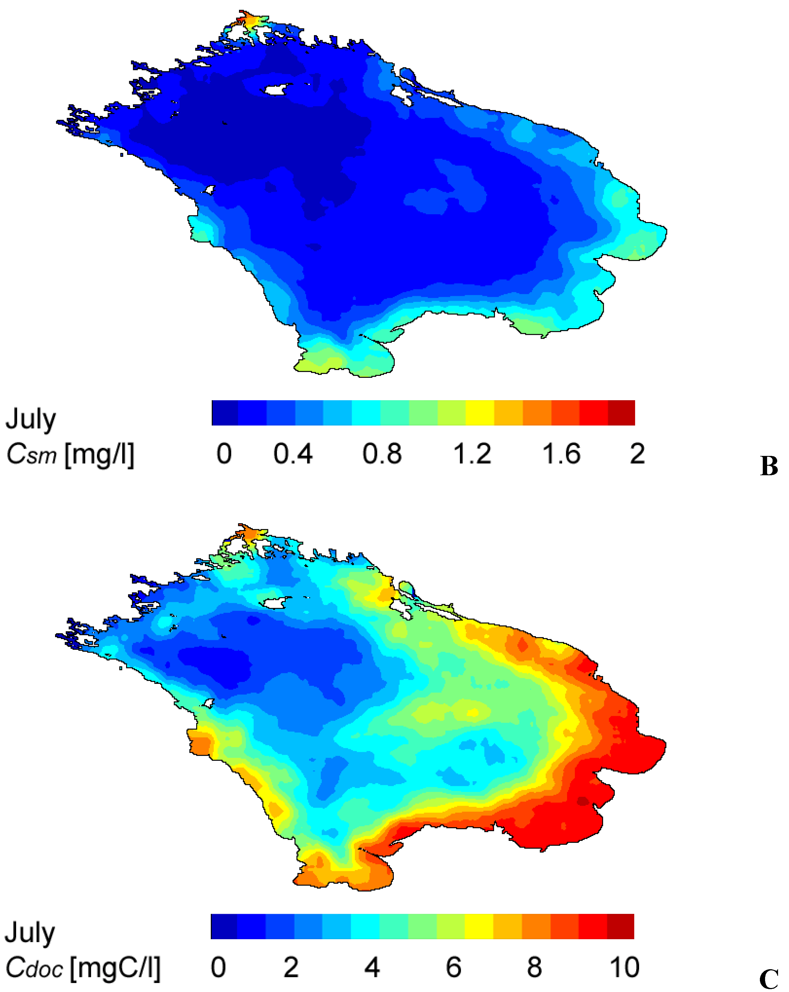
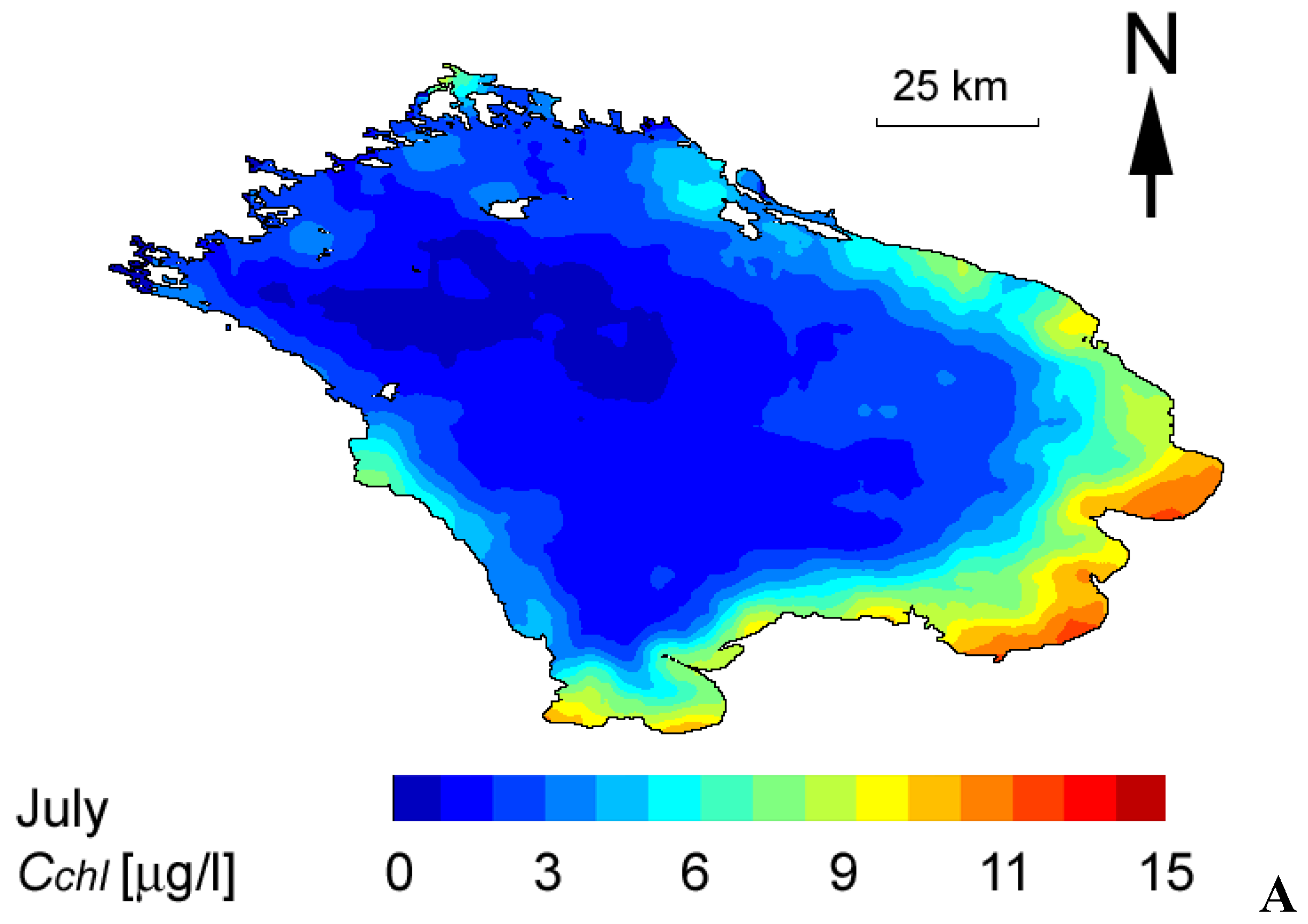
The performance of the retrieval algorithm and the hydro-optical model for Lake Ladoga is illustrated on distributions of the chl, sm and doc concentrations in Lake Ladoga (Figure 4). These results are retrieved from c.a. 400 SeaWiFS images taken during the period 1998-2004 in July and averaged.

Figure 4. Distributions of the chl (A), sm (B) and doc (C) concentrations in Lake Ladoga in July as retrieved from SeaWiFS data and averaged over 1998-2004. The maps are given in the geographic projection.

Figure 4. Distributions of the chl (A), sm (B) and doc (C) concentrations in Lake Ladoga in July as retrieved from SeaWiFS data and averaged over 1998-2004. The maps are given in the geographic projection.

The retrieved concentrations of chl, sm and doc are in compliance with the historical data from Lake Ladoga [25,26,27]. In mid-summer, the concentration of chl in Lake Ladoga, which is presently a mesotrophic water body, may vary within the range 1-25 μg/L. The central and northern parts of Lake Ladoga are deep and remain rather cold even in July. As a result, the chl concentrations are lower there than they are in shallow/well-warmed areas. This is especially so in the southern zone.

The lake water is also rich in doc: in near shore regions C_doc can be as high as 10-13 mgC/L, and on average is about 8 mgC/L [25].

Near-shore waters of Lake Ladoga also contain, although in moderate amounts, terrigenous sm brought in with river discharge. The largest rivers discharging into the lake are located in the south-eastern area (the lower right-hand part of Fig. 4), but there is also an inflow of riverine waters along the western shore (left-hand side of Fig. 4).

The central/deep regions of Lake Ladoga generally contain low amounts of sm unless temporarily persistent winds and/or meandering currents transport suspended mineral matter offshore [27,28]. All these features can be found in the CPA distributions given in Fig. 4, and this can be considered as a qualitative substantiation of the retrieved spatial distributions of chl, sm and doc in Lake Ladoga.

Thus, the above indirect verification is clearly indicative that the algorithm restores correctly the spatial distribution of chl, sm and doc in accordance with the trophic status, bathymetry and hydrology of Lake Ladoga.

3.2. White Sea (southern bays)

The White Sea, morphologically a shelf marine basin is located on the periphery of the Arctic Ocean to which it is connected through the Barents Sea. It is essentially a mediterranean sea, being semi-enclosed by the northern European landmass. Both climate change, specific landscape features of the watershed and intensification of agricultural/industrial activities in the area brought about some significant ecological changes in the sea, notably in its southern bays, which trophic status turned to mesotrophic.

Concentrations of chl, sm and doc were measured in situ in the southern bays of the White Sea (recipients of full-flowing riverine fresh waters) in July 2001. One SeaWiFS image taken synchronously with shipborne measurements on July 10, 2001 (time gaps between in situ measurements and satellite overpass were less than 24 hrs) was processed by the LM-algorithm. In the absence of a dedicated hydro-optical model, the Lake Ladoga model has been employed for reasons given in section 2.5.

The CPA concentrations measured in situ are compared in Table 4 with the concentrations retrieved by the LM–based algorithm described above.

Table 4. Comparison of the WQP concentrations measured in situ and retrieved by the LM-based algorithm from SeaWiFS data for the White Sea, Onega Bay, July 2001.

In situ measurements			Remote sensing data
chl, μg/L	doc, mgC/L	sm, mg/L	chl, μg/L	doc, mgC/L	sm, mg/L
1.6	8.3	0.25	1.3	6.5	0.8
1.1	5.8	0.25	1.2	5.5	0.7
1.1	5.9	0.65	1.1	4.5	1.1
1.5	5.8	0.70	1.5	4.0	1.0
1.8	6.3	0.30	1.6	4.0	1.0
1.8	5.3	0.10	1.7	3.9	0.9
r			0.90	0.79	0.65
RMSE			0.15	1.6	0.56

Table 4. Comparison of the WQP concentrations measured in situ and retrieved by the LM-based algorithm from SeaWiFS data for the White Sea, Onega Bay, July 2001.

In situ measurements			Remote sensing data
chl, μg/L	doc, mgC/L	sm, mg/L	chl, μg/L	doc, mgC/L	sm, mg/L
1.6	8.3	0.25	1.3	6.5	0.8
1.1	5.8	0.25	1.2	5.5	0.7
1.1	5.9	0.65	1.1	4.5	1.1
1.5	5.8	0.70	1.5	4.0	1.0
1.8	6.3	0.30	1.6	4.0	1.0
1.8	5.3	0.10	1.7	3.9	0.9
r			0.90	0.79	0.65
RMSE			0.15	1.6	0.56

3.3. Eastern Gulf of Finland

The eastern margins of the Gulf of Finland are known to be eutrophic and laden both with doc and sm [29]. Thus, these are typical case 2 waters. Like in the case of the White Sea, we lacked the Gulf of Finland inherent hydro-optical model and the Lake Ladoga model has been employed. Thus again we assumed their hydro-optical models to be very close based on the argumentation presented in Subsection 2.4.

Concentrations of chl, sm and doc were measured in the eastern Gulf of Finland on August 20, 21, 22 and 23 2002. A SeaWiFS image taken on August 20, 2002 was processed with the LM-algorithm. In situ data from stations taken on August 20 and 21 were compared with the respective remote sensing data (Table 5). The temporal mismatch (ΔT) between shipborne measurements and satellite (SeaWiFS) overflights varied been several hours (for three points) and 1 day.

Table 5. Comparison of WQP concentrations measured in situ and retrieved from SeaWiFS data for the Baltic Sea, eastern Gulf of Finland, August 2002.

Time gap	In situ measurements			Remote sensing data
	chl, μg/L	doc, mgC/L	sm, mg/L	chl, μg/L	doc, mgC/L	sm, mg/L
ΔT< 24 hrs	4.23	10.5	0.8	5.2	14.2	0.5
	9.00	12.0	1.1	12.0	14.8	2.7
	17.89	13.5	4.5	12.1	14.7	3.2
	r			0.77	0.77	0.69
	RMSE			3.8	2.7	1.2
24 hrs < ΔT < 48 hrs	15.18	14.3	3.1	13.5	14.9	1.1
	7.32	9.0	0.9	18.6	14.7	1.9
	13.12	8.6	0.9	18.0	14.8	2.3
	9.97	8.3	1.0	18.0	7.3	1.1
	7.31	8.3	1.2	8.1	9.0	1.5
	7.58	7.9	0.8	10.0	8.1	1.3
	r			0.29	0.56	-0.46
	RMSE			6.1	3.4	1.1

Table 5. Comparison of WQP concentrations measured in situ and retrieved from SeaWiFS data for the Baltic Sea, eastern Gulf of Finland, August 2002.

Time gap	In situ measurements			Remote sensing data
	chl, μg/L	doc, mgC/L	sm, mg/L	chl, μg/L	doc, mgC/L	sm, mg/L
ΔT< 24 hrs	4.23	10.5	0.8	5.2	14.2	0.5
	9.00	12.0	1.1	12.0	14.8	2.7
	17.89	13.5	4.5	12.1	14.7	3.2
	r			0.77	0.77	0.69
	RMSE			3.8	2.7	1.2
24 hrs < ΔT < 48 hrs	15.18	14.3	3.1	13.5	14.9	1.1
	7.32	9.0	0.9	18.6	14.7	1.9
	13.12	8.6	0.9	18.0	14.8	2.3
	9.97	8.3	1.0	18.0	7.3	1.1
	7.31	8.3	1.2	8.1	9.0	1.5
	7.58	7.9	0.8	10.0	8.1	1.3
	r			0.29	0.56	-0.46
	RMSE			6.1	3.4	1.1

3.4. North Sea

For the LM-based algorithm validation, 20 HPLC chl and Ferrybox turbidity (tsm) samples have been available. These parameters were measured using the NIVA Ferrybox system [30] onboard the passenger ferry MS Color Festival that was crossing the Skagerrak (eastern-most region of the North Sea) between Oslo (Norway) and Fredrikshavn (Denmark) twice per day. For HPLC chl determination water samples were collected and analysed in the laboratory. In addition, the Ferrybox system measured chl fluorescence and turbidity continuously along the entire ferry transect. The turbidity data were converted to tsm and used in the validation as single point measurements coincident with the HPLC match-up locations. Data used for this study originated from 9 different dates through March to November, 2007. A comparison of concentrations of chl and tsm measured in situ and retrieved by our LM-based algorithm from the MERIS data (Table 6) indicates that the LM-based algorithm provides a high level of correlation (0.89) between the retrieved and measured values for chl and significantly less high, but still acceptable (0.46), for tsm with the RMSE of about 1.0 and 0.47 respectively.

Table 6. Comparison of WQP concentrations measured in situ and retrieved from MERIS data for the North Sea, Skagerrak, 2007 with the LM-algorithm and standard ESA algorithms.

In situ measurements		Remote sensing data
		LM - algorithm		ESA standard algorithms
chl, µg/L	tsm, mg/L	chl, µg/L	sm, mg/L	algal_1, mgC/L	algal_2, mgC/L
0.76	0.75	1.29	1.02	1.11	1.24
0.72	1.08	0.93	1.29	1.85	2.22
0.49	1.10	1.63	1.02	1.49	2.14
0.96	0.84	0.95	0.67	1.92	2.30
0.61	1.04	1.94	0.89	1.24	2.07
11.06	2.49	8.47	2.10	11.35	13.61
2.68	1.24	2.25	2.18	2.57	5.50
5.55	2.35	6.25	2.31	6.36	9.13
0.56	0.95	1.58	0.88	0.83	2.39
4.13	1.14	3.89	2.18	3.97	6.83
0.81	0.85	0.52	1.25	1.04	0.90
3.84	1.16	3.81	1.67	3.69	5.30
5.6	2.13	7.32	1.72	10.18	8.49
1.09	0.90	1.60	1.08	0.72	2.30
4.1	1.15	4.30	1.64	4.11	5.70
0.51	0.94	1.04	0.87	1.99	3.19
0.73	0.76	0.38	0.77	1.20	1.39
4.04	1.16	3.86	1.91	3.56	5.91
9.03	2.35	7.90	1.80	10.56	10.95
r		0.96	0.68	0.95	0.98
RMSE		0.95	0.46	1.27	2.10

Table 6. Comparison of WQP concentrations measured in situ and retrieved from MERIS data for the North Sea, Skagerrak, 2007 with the LM-algorithm and standard ESA algorithms.

In situ measurements		Remote sensing data
		LM - algorithm		ESA standard algorithms
chl, µg/L	tsm, mg/L	chl, µg/L	sm, mg/L	algal_1, mgC/L	algal_2, mgC/L
0.76	0.75	1.29	1.02	1.11	1.24
0.72	1.08	0.93	1.29	1.85	2.22
0.49	1.10	1.63	1.02	1.49	2.14
0.96	0.84	0.95	0.67	1.92	2.30
0.61	1.04	1.94	0.89	1.24	2.07
11.06	2.49	8.47	2.10	11.35	13.61
2.68	1.24	2.25	2.18	2.57	5.50
5.55	2.35	6.25	2.31	6.36	9.13
0.56	0.95	1.58	0.88	0.83	2.39
4.13	1.14	3.89	2.18	3.97	6.83
0.81	0.85	0.52	1.25	1.04	0.90
3.84	1.16	3.81	1.67	3.69	5.30
5.6	2.13	7.32	1.72	10.18	8.49
1.09	0.90	1.60	1.08	0.72	2.30
4.1	1.15	4.30	1.64	4.11	5.70
0.51	0.94	1.04	0.87	1.99	3.19
0.73	0.76	0.38	0.77	1.20	1.39
4.04	1.16	3.86	1.91	3.56	5.91
9.03	2.35	7.90	1.80	10.56	10.95
r		0.96	0.68	0.95	0.98
RMSE		0.95	0.46	1.27	2.10

It is worthwhile to compare the efficiency of the developed LM-based algorithm with the efficiency of other algorithms suggested for MERIS data processing (Table 6). Algal_1 and algal_2 are the products of standard ESA algorithms for estimation of the chl concentration in, respectively, oceanic (case 1) and coastal (case 2) waters.

As Table 6 indicates, the LM-based algorithm with the developed dedicated hydro-optical model performs appreciably better, both in terms of the explained variance and RMSE as compared not only with the oceanic algal-1 but also the coastal algal-2 algorithm. A validation of the MERIS standard products and some other alternative algorithms has been conducted recently by [31].

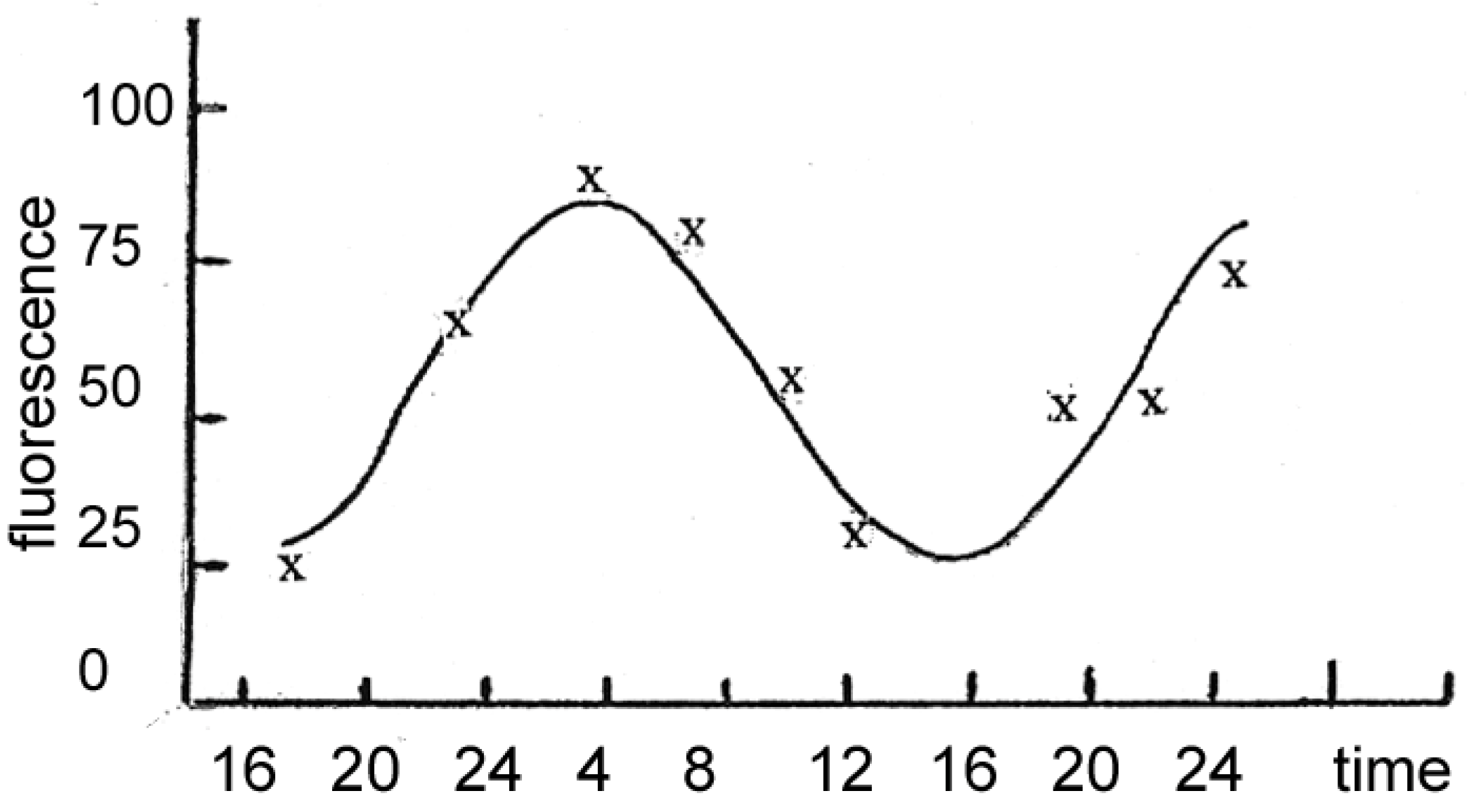
As an alternative approach for evaluating the performance of the LM-based algorithm, the values of phytoplankton chlorophyll fluorescence measured by the Ferrybox system were used to estimate a proxy for the chlorophyll concentration (chl_F) along the whole transect using a linear regression between concurrent measurements of HPLC chl and sensor chl fluorescence. It is important to note that the use of chl_F do not qualify for a proper validation of the satellite chl products, as the conversion factor between chl concentration and chl fluorescence varies due to a number of factors. However, chl_F provides important information about the variation and gradients of phytoplankton activity along the ferry transect. The relative agreement between the satellite product and the in situ observations along the transect can thus be studied.

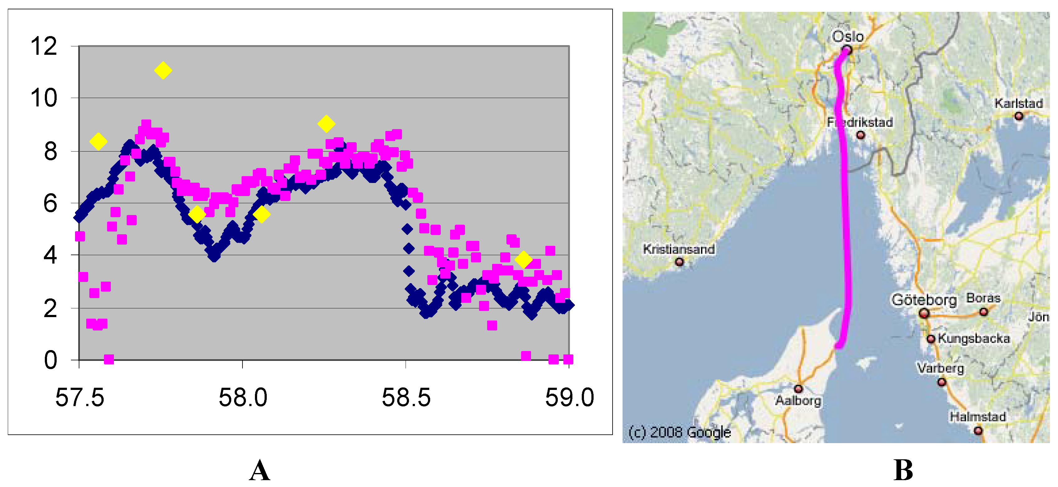
Our comparison shows (Figure 5) that chl concentrations retrieved with the LM algorithm are rather close to the chl_F values derived from the night-time fluorescence signals (r = 0.83, RMSE = 2.7 μg/L) and compare worse with the chl_F values derived from the day-time fluorescence signals (r = 0.48, RMSE 8.85 μg/L).

Figure 5. A) Comparison of FerryBox nigh-time chl_F (blue dots) with the results of chl retrieval with the LM-based algorithm (pink dots) and HPLC measurements (yellow dots) taken on 25.03.2007 along the transect running between Oslo, Norway and Hirtshals, Denmark. Axes: on the horizontal – latitude, °N, on the vertical - chl concentration (μg/L). B) Location of the transect between Oslo and Fredrikshavn.

Figure 5. A) Comparison of FerryBox nigh-time chl_F (blue dots) with the results of chl retrieval with the LM-based algorithm (pink dots) and HPLC measurements (yellow dots) taken on 25.03.2007 along the transect running between Oslo, Norway and Hirtshals, Denmark. Axes: on the horizontal – latitude, °N, on the vertical - chl concentration (μg/L). B) Location of the transect between Oslo and Fredrikshavn.

Great Laurentian Lakes

3.5. Lake Michigan

Lake Michigan is the second largest of North America’s Great Lakes and the largest freshwater lake in the United States. It is an oligotrophic water body with some eutrophicated areas (like Green Bay and the eastern coastal zone).

A small-scale shipborne campaign was performed for validation purposes by ERIM. Values of chl, tsm and toc concentrations were measured at 13 stations near the lake eastern coast in July 2003. By definition, tsm encompasses all suspended matter including both mineral and organic fractions. Obviously, correspondence between sm and tsm can be poor, for instance, under conditions of an enhanced growth of phytoplankton. By definition, toc encompasses both particulate and dissolved fraction of organic carbon [32], therefore correspondence between doc and toc can also be poor.

SeaWiFS images taken synchronously with shipborne measurements were processed by the LM-algorithm. The time gap between remote and in situ measurements did not exceed 24 hrs. As there was no a dedicated hydro-optical model for Lake Michigan, the hydro-optical model of Lake Ontario was tentatively chosen. Table 7 lists the measured and retrieved values of concentrations.

Table 7. Comparison of CPA concentrations measured in situ and retrieved from SeaWiFS data from the eastern coast of Lake Michigan, July 2003; tsm– total (i.e. organic and inorganic) suspended matter, toc– total (i.e. suspended and dissolved) organic carbon.

In situ measurements			Remote sensing data
chl, µg/L	tsm, mg/L	toc, mgC/L	chl, µg/L	sm, mg/L	doc, mgC/L
0.72	2.42	24.63	1.11	10.17	23.86
1.2	1.34	22.19	1.85	9.81	24.37
0.5	4.38	15.96	0.46	2.58	10.12
0.46	1.65	37.73	0.44	3.91	24.37
0.53	9.38	4.98	0.5	4.43	7.32
0.63	1.36	8.45	0.57	2.76	7.89
0.55	2.68	18.63	0.42	2.55	11.14
0.54	1.45	7	0.2	1.3	4.8
0.63	5.33	9.55	0.08	1.53	5.71
0.71	3.95	7.71	0.12	1.19	4.51
0.51	0.72	24.07	0.21	1.36	15.08
r			0.82	-0.09	0.88
RMSE			0.36	4.1	5.9

Table 7. Comparison of CPA concentrations measured in situ and retrieved from SeaWiFS data from the eastern coast of Lake Michigan, July 2003; tsm– total (i.e. organic and inorganic) suspended matter, toc– total (i.e. suspended and dissolved) organic carbon.

In situ measurements			Remote sensing data
chl, µg/L	tsm, mg/L	toc, mgC/L	chl, µg/L	sm, mg/L	doc, mgC/L
0.72	2.42	24.63	1.11	10.17	23.86
1.2	1.34	22.19	1.85	9.81	24.37
0.5	4.38	15.96	0.46	2.58	10.12
0.46	1.65	37.73	0.44	3.91	24.37
0.53	9.38	4.98	0.5	4.43	7.32
0.63	1.36	8.45	0.57	2.76	7.89
0.55	2.68	18.63	0.42	2.55	11.14
0.54	1.45	7	0.2	1.3	4.8
0.63	5.33	9.55	0.08	1.53	5.71
0.71	3.95	7.71	0.12	1.19	4.51
0.51	0.72	24.07	0.21	1.36	15.08
r			0.82	-0.09	0.88
RMSE			0.36	4.1	5.9

3.6. Lake Huron

Lake Huron is oligotrophic in its most areas, except for Saginaw Bay and the southern Georgian Bay where eutrophic conditions prevail [33]. The Saginaw Bay water quality is largely controlled by run-off, tributary discharge, as well as by anthropogenic effluents coming from Bay City and the city of Saginaw. The phytoplankton species for the Huron Lake open area are typical of oligotrophic water bodies. In contrast, the phytoplankton community in Saginaw Bay is representative of typical eutrophic conditions [33].

The above indicates that there should be two distinctly different water masses residing in the outer and inner parts of the Bay which is conducive to a substantial difference in the optical characteristics of both parts of the Bay due to differences in the phytoplankton abundance and taxonomic composition, mineralogical and microphysical characteristics of suspended minerals. The suspended matter in the inner part should be directly provided by nearby tributaries, run-off and wind/water dynamics-driven resuspension whereas in the outer part it is largely the result of filtering due to gravitational settling of the particulate matter generated by distant sources).

Similar considerations could be suggested with regard to the dissolved organics (doc): the autochthonous component in the outer part of the bay could be predominant, whereas in the inner part the allochthonous component should most certainly prevail. Evidently, under appropriate conditions, due to wind and current impacts, both types of water masses can invade the counterparts of the bay and mix up with the ambient waters.

Field studies on the Great Laurentian Lakes were performed by ERIM in June and July 1998 at 13 stations in the inner and outer parts of Saginaw Bay. Conducted from board a small research vessel, spectrometric measurements and CPA sampling for chl, and doc were performed. The spectrometric measurements (at the SeaWiFS wavelengths) allowed retrieving spectral volume reflectance, R(λ, Ө₀).

The LM algorithm was applied for retrieval of WQP concentrations from spectra of R(λ, Ө₀) several times with different hydro-optical models. The test showed that for the inner and outer parts of the bay the most suitable hydro-optical models are that of Lake Ladoga and slightly modified [34] Ontario model [33], respectively (Table 8). The retrieved sm values appear as quite plausible in view of the typical Secchi disc depths (averaging 1-3 m, [33]).

Table 8. Comparison of chl and doc concentrations measured in situ and retrieved from optical measurements in Lake Huron. The first part of the table corresponds to measurements in the Saginaw Bay, the second one – outer part of the lake. The sm retrievals are not supported by in situ determinations.

Model	In situ measurements		Remote sensing data
	chl, mg/L	doc, mgC/L	chl, mg/L	doc, mgC/L	sm, mg/L
Lake Ladoga	14.24 ±2.14	2.45 ±0.26	12.56 ±3.28	2.68 ±0.56	0.72
	9.98 ±1.5	2.73 ±0.27	12.62 ±2.30	1.76 ±0.63	2.49
	13.73 ±2.06	3.17 ±0.32	9.75 ±3.16	3.95 ±0.73	3.83
	10.05 ±1.51	2.35 ±0.24	10.47 ±2.31	4.75 ±0.54	3.11
	17.26 ±2.59	2.39 ±0.24	19.87 ±3.97	1.7 ±0.55	3.21
Lake Ontario	1.26 ±0.19	1.48 ±0.15	2.23 ±0.29	1.04 ±0.34	0.14
	0.79 ±0.12	2.07 ±0.21	0.93 ±0.18	2.71 ±0.48	0.19
	1.13 ±0.17	1.14 ±0.11	0.88 ±0.25	0.59 ±0.26	0.1
	1.28 ±0.19	1.47 ±0.15	0.89 ±0.29	1.12 ±0.34	0.18
	1.74 ±0.26	2.27 ±0.23	2.11 ±0.40	2.6 ±0.52	0.23
	0.35 ±0.5	1.56 ±0.16	0.24 ±0.08	1 ±0.35	0.1
	0.51 ±0.8	1.47 ±0.15	0.88 ±0.12	1.13 ±0.34	0.12
	0.8 ±0.12	2.03 ±0.2	0.88 ±0.18	1 ±0.47	0.11
r			0.96	0.71
RMSE			1.6	0.93

Table 8. Comparison of chl and doc concentrations measured in situ and retrieved from optical measurements in Lake Huron. The first part of the table corresponds to measurements in the Saginaw Bay, the second one – outer part of the lake. The sm retrievals are not supported by in situ determinations.

Model	In situ measurements		Remote sensing data
	chl, mg/L	doc, mgC/L	chl, mg/L	doc, mgC/L	sm, mg/L
Lake Ladoga	14.24 ±2.14	2.45 ±0.26	12.56 ±3.28	2.68 ±0.56	0.72
	9.98 ±1.5	2.73 ±0.27	12.62 ±2.30	1.76 ±0.63	2.49
	13.73 ±2.06	3.17 ±0.32	9.75 ±3.16	3.95 ±0.73	3.83
	10.05 ±1.51	2.35 ±0.24	10.47 ±2.31	4.75 ±0.54	3.11
	17.26 ±2.59	2.39 ±0.24	19.87 ±3.97	1.7 ±0.55	3.21
Lake Ontario	1.26 ±0.19	1.48 ±0.15	2.23 ±0.29	1.04 ±0.34	0.14
	0.79 ±0.12	2.07 ±0.21	0.93 ±0.18	2.71 ±0.48	0.19
	1.13 ±0.17	1.14 ±0.11	0.88 ±0.25	0.59 ±0.26	0.1
	1.28 ±0.19	1.47 ±0.15	0.89 ±0.29	1.12 ±0.34	0.18
	1.74 ±0.26	2.27 ±0.23	2.11 ±0.40	2.6 ±0.52	0.23
	0.35 ±0.5	1.56 ±0.16	0.24 ±0.08	1 ±0.35	0.1
	0.51 ±0.8	1.47 ±0.15	0.88 ±0.12	1.13 ±0.34	0.12
	0.8 ±0.12	2.03 ±0.2	0.88 ±0.18	1 ±0.47	0.11
r			0.96	0.71
RMSE			1.6	0.93

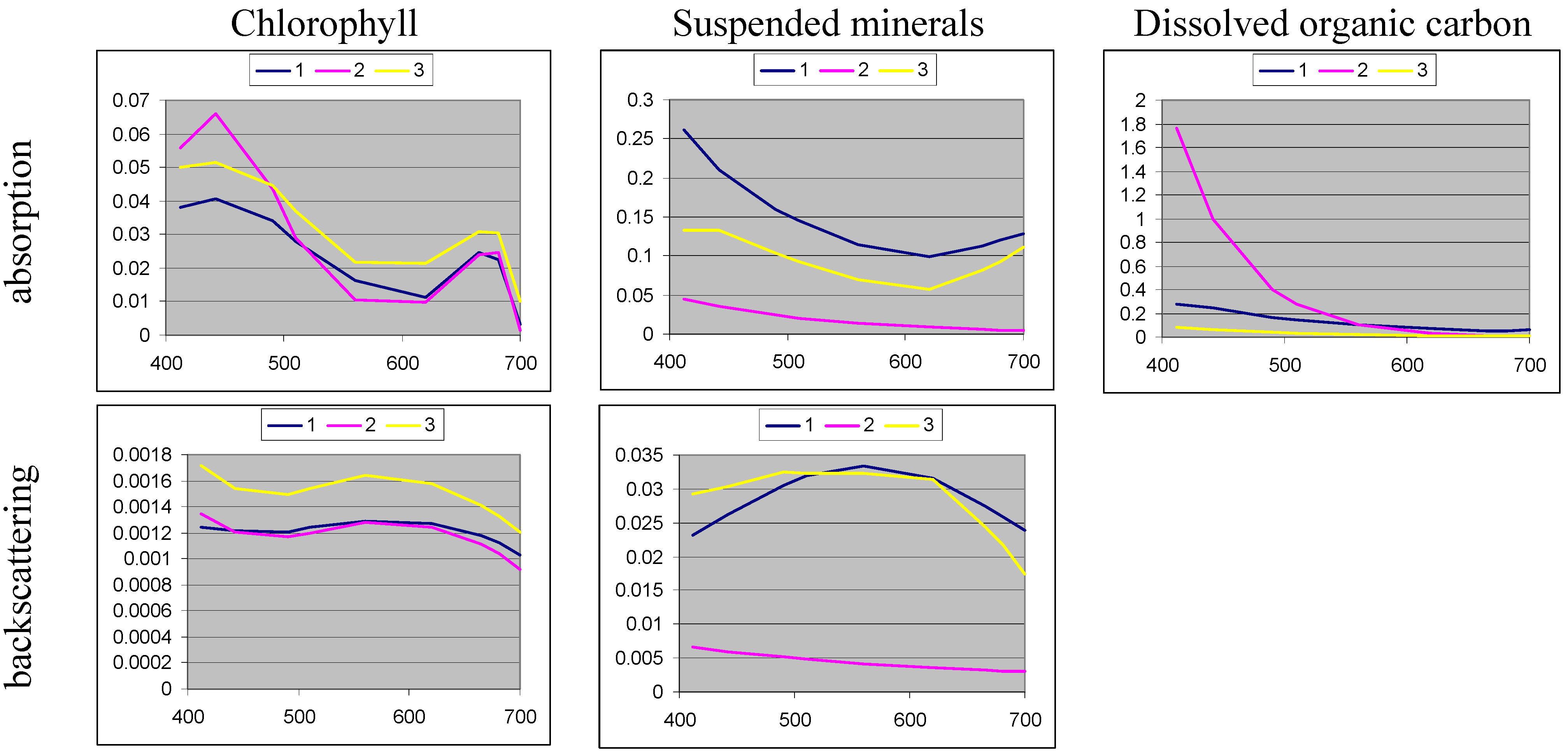
This experiment is indicative that very time consuming and expensive determinations of spectral specific coefficients of absorption, a*(λ) and backscattering, b_b*(λ) in some cases can be replaced by less cumbersome measurements of both the concentration vector C(chl, sm, doc) and spectral volume reflectance, R(λ) or subsurface spectral remote sensing reflectance, R_rsw(λ).

3.7. Bay of Biscay

The Bay of Biscay is an area of incursion of the North Atlantic waters into the western periphery of the European continent. It resembles a gigantic triangular, which is a recipient of numerous rivers, some of them being fairly full-flowing and bringing large amounts of suspended minerals, dissolved organic matter and nutrients into the bay. In the spatial distribution of the terrigenous suspended and dissolved matter, the important role is played by fronts of various nature, in particular the thermo-haline front forming over the 100 m isobath. The coastal zone is conditionally bounded by the 200 m isobath, beyond which the pelagic zone extends out to the western boundary of the bay. The phytoplankton community within the coastal zone is mostly controlled by diatoms [35].

In the Bay of Biscay not only the coastal zone should be considered as the area of case 2 waters. The pelagic zone is known to be the realm of extensive blooms of a coccolithophore, Emiliania Huxley, which usually accounts for about 90% the phytoplankton, whereas the remaining ~10% is the portion of diatoms.

Coccolithophores are algal cells covered with calcium carbonate plates that, at the late phase of the algal life-cycle, become detached completely or partially from the cell’s body. It implies that the algal chl within the blooming areas generally does not correlate with this mineral residue. Hence, by definition (see Introduction), such waters subsume under the category of case 2 waters.

We applied our LM-based algorithm to satellite data (SeaWiFS, MODIS, MERIS) collected over the Bay using two separate hydro-optical models: one for the coastal zone and one for the pelagic waters.

The first hydro-optical model was obtained through multivariate optimization of the North Sea hydro-optical model. The optimization approach is similar to the one described in the section 2.5. This hydro-optical model considered chl, tsm and yellow substance (cdom) as CPAs.

For validation of the LM-algorithm we utilised the database of in situ and SeaWiFS data matchups developed at IFREMER, Brest, France [36]. The database consists of more than 500 simultaneous chl and tsm measurements collected synchronously with SeaWiFS overflights during 6 years (1998 – 2004) on several tens of stations along the French coast of the Bay of Biscay and during several expeditions to the centre of the bay.

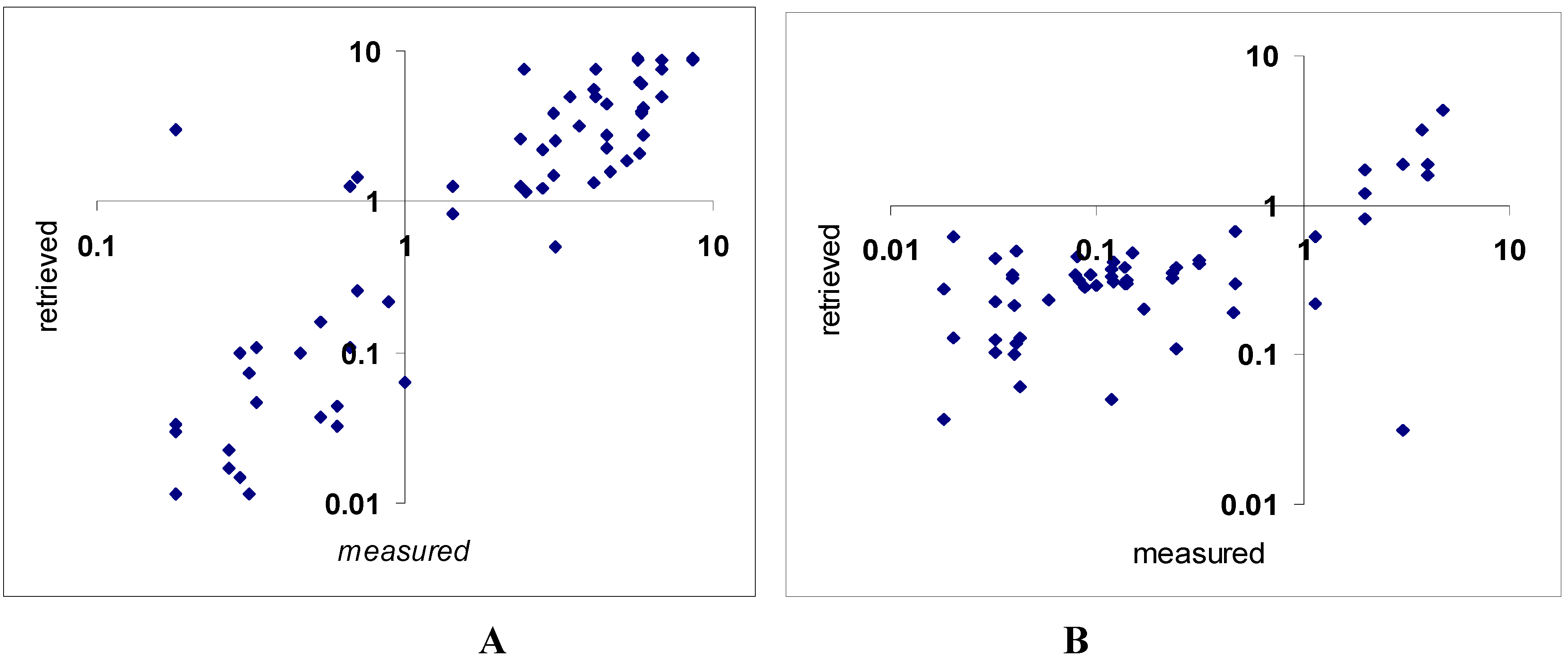
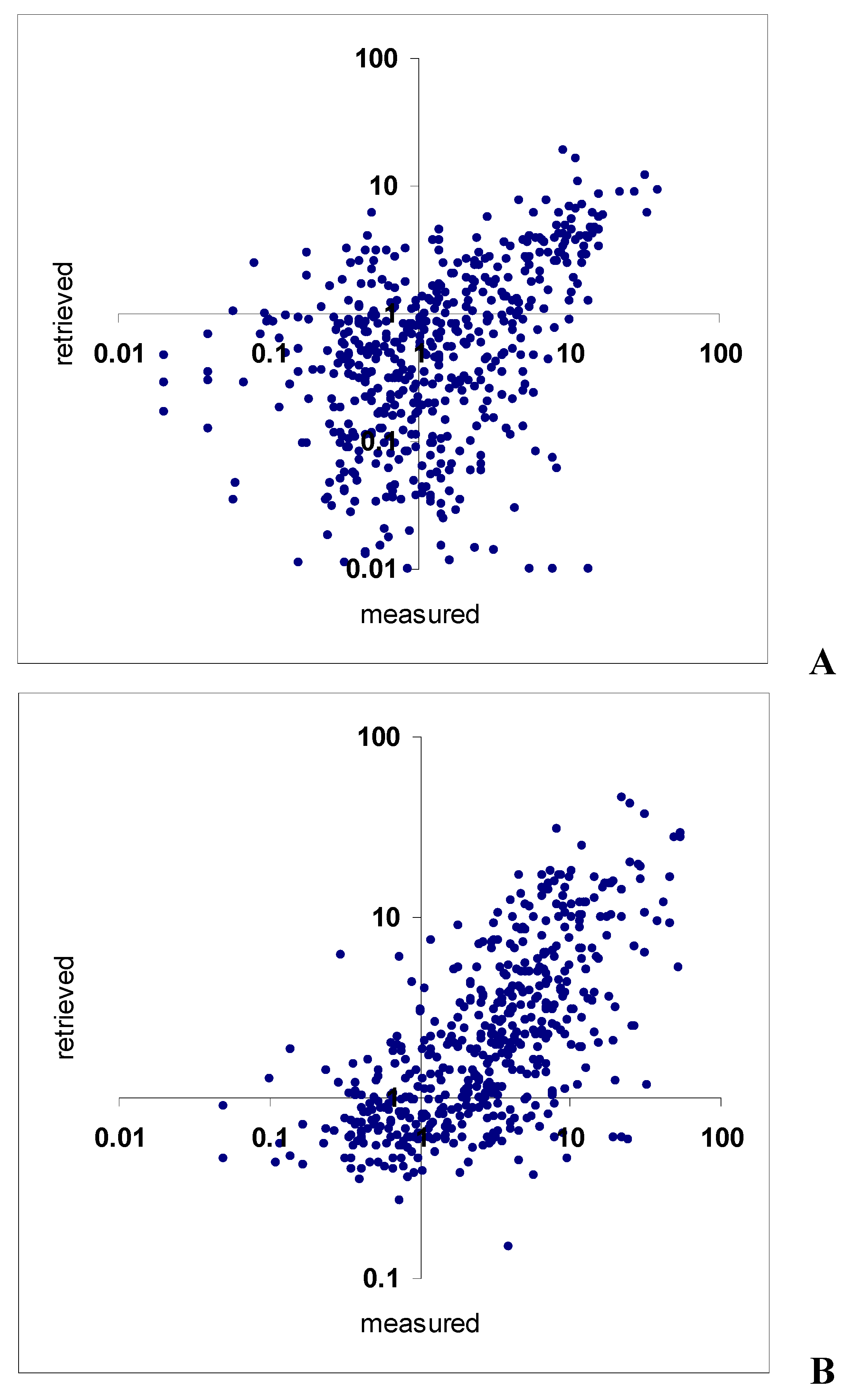
Our comparison of chl and tsm obtained by applying the LM-based algorithm to R_rsw(λ) measured remotely showed (Fig. 6) that correlation is high (r_chl = 0.67, r_sm = 0.60), absolute difference is low (RMSE_chl = 3.7 μg/L, RMSE_sm = 6.6 mg/L) and the retrieved values are slightly overestimated (chl_retrieved = 0.3 chl_measured + 0.4, sm_retrieved = 0.4 chl_measured + 1.5) indicating that the established dependence is governed exclusively by the parameter in question.

The second hydro-optical model applied for the Bay of Biscay assumes coccolithophores, coccoliths and diatoms as CPAs in the pelagic waters (here, the symbol λ denoting wavelength dependence is dropped for simplicity):

a = a_w+a*_php·C_php+a*_coc·C_coc+a* _cc·C_cc+a*_sm·C_sm+a*_cdom·C_cdom;

(9)

b_b = b_bw+b_b*_php·C_php+ b_b*_coc ·C_coc+b_b*_cc·C_cc+b_b*_sm,·C_sm,

(10)

where indices w, php, coc and cc refer to water, diatom phytoplankton, coccolithophores and coccoliths, respectively. The specific absorption coefficient of coccoliths, a*_cc can be assumed zero because coccoliths practically do not absorb light. The coccolithophore spectral coefficients a*_coc and b_b*_coc were taken from [37,38,39].

Figure 6. Comparison of chl (A) and tsm (B) concentrations measured in situ and retrieved from remote sensing data obtained for the coastal zone of the Biscay Bay for the time period 1998 – 2004.

Figure 6. Comparison of chl (A) and tsm (B) concentrations measured in situ and retrieved from remote sensing data obtained for the coastal zone of the Biscay Bay for the time period 1998 – 2004.

Thus, the second algorithm is intended not only to flag the coccolithophore blooming areas, but also to differentiate chl in diatoms and coccolithophores as well as to quantify the concentration of coccoliths.

The spatial distributions of chl, cdom and tsm (not illustrated here) retrieved with the LM-algorithm explicitly exhibit the impact of the river discharge along the coastline, especially in the area adjacent to the estuaries of Rivers Loire and Gironde, the most full-flowing on the French seaboard.

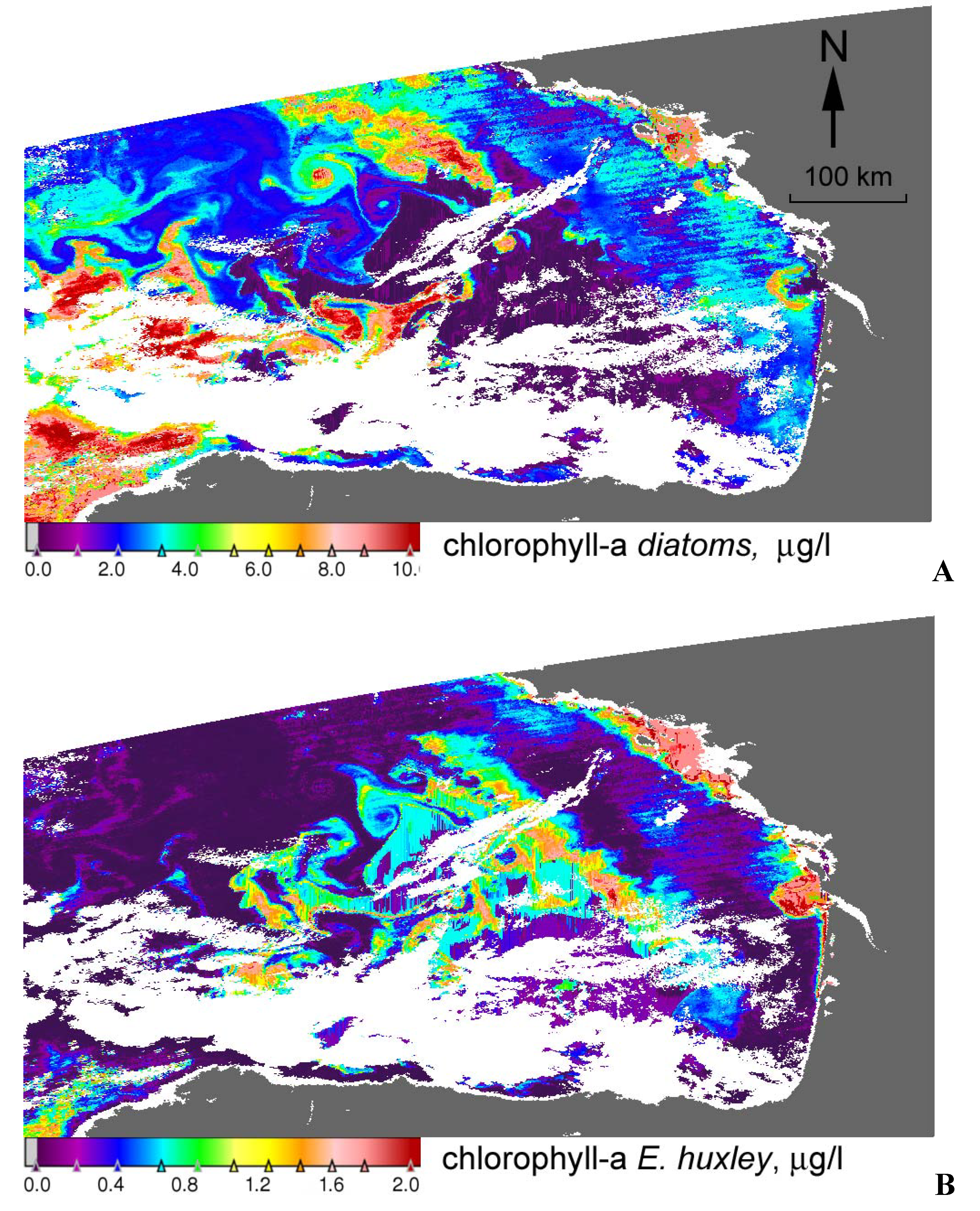
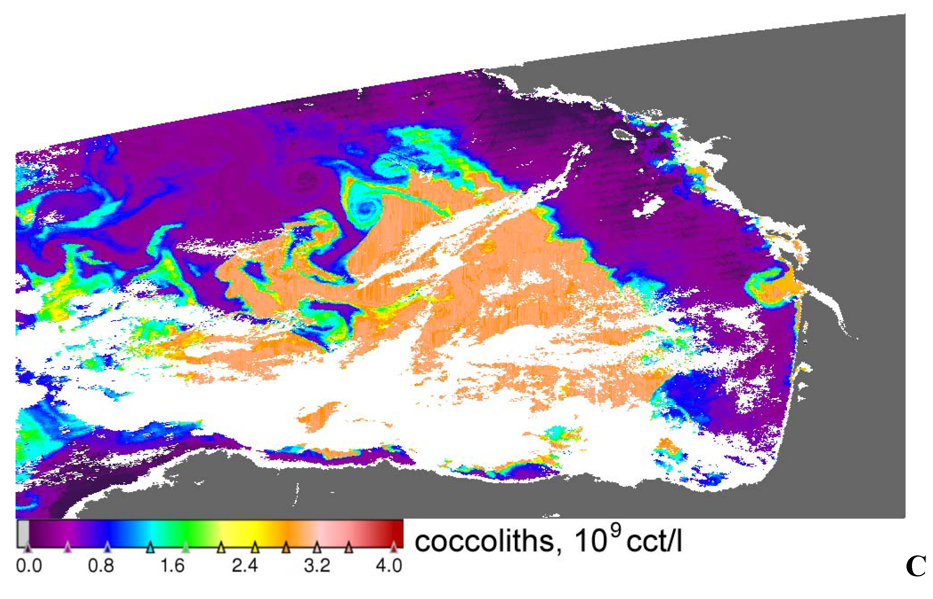
Validation of the algorithm might be done through the analysis of spatial distributions of coccolithophores, coccoliths, and diatoms (Figure 7). As seen, in 2005 there was a very extensive coccolithophore bloom covering most of the pelagic area, but in the coastward direction it is distinctly restricted by the 200 m isobath that corresponds to a sharp shelf break. This is a clear manifestation of the importance of the bay’s hydrography, and the influence of the associated fronts mentioned above.

Importantly, inasmuch as the employed algorithm yields the concentrations of coccoliths, it was possible to assess the content of suspended carbon in the surface layer. It is known that the mean concentration of carbon in a coccolith is about 0.2·10^-12 g [40]. For the situation exemplified in Fig. 7, the area occupied by the E. Huxley mounted up to 800 km². With the thickness of the mixing layer equaling 10 m, the entire volume in question makes up 8·10¹¹ m³. The mean concentration of coccoliths as determined from the satellite image constituted 8·10¹² coccoliths/m³. Thus, the total amount of inorganic carbon in the plume was assessed at 17·10¹² g. Such assessments are important in light of the global carbon’s role in the climate status of the planet [40].

Figure 7. Retrieval of spatial distributions of chl of diatoms (A) and E. huxley (B) as well as coccoliths (C) from a MODIS image taken on 5 May, 2005 over the Bay of Biscay. The maps are given in the geographic projection.

Figure 7. Retrieval of spatial distributions of chl of diatoms (A) and E. huxley (B) as well as coccoliths (C) from a MODIS image taken on 5 May, 2005 over the Bay of Biscay. The maps are given in the geographic projection.

4. Discussion

4.1. Error sources analysis

As seen in Section 2.5, the pivotal element of the developed algorithm is the employed hydro-optical model, so that the accuracy of the concentration vector retrieval is controlled (apart from the atmospheric correction) by the adequacy of that model. Bearing in mind that the employed hydro-optical model has been specifically developed only for one water body, and further tentatively used for another one (as in the case of the White Sea, Gulf of Finnland, Lake Michigan or Lake Huron), it would hardly be reasonable to expect a closer correspondence between the in situ and retrieved data.

Despite a frequent lack of synchronality between shipborne measurements and satellite overflights (Δt sometimes surpassed 10 hours), the retrieved and measured data compare pretty well as is illustrated in Table 4, Table 5, Table 6, Table 7 and Table 8. The closest conformity between these sets of data is observed for the coinciding dates when there is a chance that the field of chl remains more or less unchanged. Conversely, this agreement deteriorates as the time difference grows.

When analysing Table 4, Table 5, Table 6, Table 7 and Table 8, it should be kept in mind that each in situ measurement relates to a single point (measuring less than 1 m by 1 m) on the water surface, whereas the satellite signal, from which the CPA concentration vector is retrieved, refers to a pixel measuring about 1 km by 1 km. Although the pixel area encompasses the point at which the in situ measurement has been performed, this fact, nevertheless, implies that the retrieved CPA concentration vector is a surface-averaged value for the processed pixel. Understandably, in the case of pronounced horizontal and vertical heterogeneity of CPA distributions (which is a very common case), the departures between the in situ measurements and retrieved CPAs are inevitable. Naturally, this applies to all intercomparison/validation case studies discussed throughout the text.

As seen, in the case of the North Sea the correlation between the retrieved chl and chl_F are significantly higher for the night-time cruises than for the day-time ones. Given that the satellite overpasses the study area at about 11 am local time, the explanation is thought to be residing in the sinusoidal diurnal cycle of the phytoplankton fluorescence (Figure 8, [41]): the fluorescence signal is minimum at the local noon, and its maximum falls on the local midnight. The ratio between chl and fluorescence varies on the same diurnal scale, due to the varying photosynthetic state of the phytoplankton cells. Thus the correlation between chl concentration measured by the satellite and fluorescence measured by the Ferrybox system varies accordingly.

Figure 8. Diurnal cycle of the phytoplankton fluorescence (0 m, relative units) recorded in the Riga Bay, May 1975 [41]; t- local time (hrs).

Figure 8. Diurnal cycle of the phytoplankton fluorescence (0 m, relative units) recorded in the Riga Bay, May 1975 [41]; t- local time (hrs).

In the Lake Michigan case study it is evident that a poorer correspondence for sm and doc is due to the fact that we had to compare them with total suspended substance (TSS), and total organic carbon (TOC) that necessarily differ from sm and doc envisaged by the Lake Ontario hydro-optical model. Obviously, correspondence between sm and tsm can be poor, for instance, under conditions of an enhanced growth of phytoplankton. By definition, toc encompasses both particulate and dissolved fraction of organic carbon [32], therefore correspondence between doc and toc can also be poor. However, even under such conditions the algorithm explains 0.83 of chl variance.

It should also be mentioned that a poorer correspondence for sm concentrations measured in the White Sea is most likely due to a filter with coarse pores used for water sample processing and sm extraction.

4.2. Concluding Remarks

An operational algorithm based on the Levenberg-Marquardt multivariate optimization technique is developed for processing remote sensing data in the visible. The algorithm allows to retrieve simultaneously the concentrations of three main colour producing agents such as phytoplankton chlorophyll, suspended minerals and dissolved organic matter. These are natural water constituents frequently considered as water quality parameters. The algorithm is outfitted with the quality control module increasing the validity of retrieval results.

The developed algorithm is neither area- nor satellite sensor- specific: indeed, the presented results explicitly indicate that SeaWiFS, MODIS and MERIS data on a variety of inland and marine coastal waters on the European and North American continent can be successfully processed by our algorithm provided with an adequate hydro-optical model. It can easily be used for processing images taken not only by any present but also future ocean colour sensors. The algorithms is intended to be utilized for processing satellite images taken over case 2 waters, for case 1 waters standard NASA and ESA algorithms are more efficient [6].

The essential element of the algorithm is the hydro-optical model, which is water-body specific. However, several examples are given how this difficulty/impediment can be overcome in specific cases. Extensive validation experiments conducted in a variety of water bodies indicate that the algorithm is robust and efficient in the case of both marine coastal and inland/lacustrine waters.

References

1. Morel, A.; Prieur, L. Analysis of variations in ocean colour. Limnol. Oceanogr. 1977, 22, 709–722. [Google Scholar] [CrossRef]
2. O’Reilly, J. E.; Maritorena, S.; Mitchell, B. G.; Siegel, D. A.; Carder, K. L.; Garver, S. A.; Kahru, M.; McClain, C. Ocean colour chlorophyll algorithms for SeaWiFS. J. Geophys. Res. 1998, 103, 2493–24953. [Google Scholar]
3. Ackleson, S. Ocean optics research at the start of the 21st century. Oceanography 2001, 22, 5–8. [Google Scholar] [CrossRef]
4. Levenberg, K. A method for the solution of certain non-linear problems in least squares. Quant. Appl. Math. 1944, 2, 164–168. [Google Scholar]
5. Marquardt, D. W. An algorithm for least-squares estimation of non-linear parameters. J. Intern. Soc. Appl. Math. 1963, 11, 36–48. [Google Scholar]
6. Morel, A.; Antoine, D. Pigment Index Retrieval In Case 1 Waters: Algorithm Theoretical Basis Document 2.9; Université Pierre Et Marie Curie: Paris, 2000; p. 26. [Google Scholar]
7. Schiller, H.; Doerffer, R. Improved Determination of Coastal Water Constituent Concentrations From MERIS Data. IEEE Trans. Geosci. Remote Sens. 2005, 43, 1585–1591. [Google Scholar] [CrossRef]
8. Atkinson, P. M.; Tatnall, A. R. T. Neural networks in remote sensing. Int. J. Rem. Sens. 1997, 18, 699–709. [Google Scholar] [CrossRef]
9. Jerome, J. H.; Bukata, R. P.; Miller, J. R. Remote sensing reflectance and its relationship to optical properties of natural water. Int. J. Rem. Sens. 1996, 17, 43–52. [Google Scholar] [CrossRef]
10. Pozdnyakov, D. V.; Grassl, H. Colour of Inland and Coastal Waters: a methodology for its interpretation; Springer-Praxis: Chichester, U.K., 2003; p. 170. [Google Scholar]
11. Press, W. H.; Teukolsky, S. A.; Vettering, W. T.; Flannery, B. P. Numerical Recipes in C: The Art of Scientific Computing 2nd ed.; Cambridge University Press: New York, 1992; p. 452. [Google Scholar]
12. Kondratyev, K. Ya.; Pozdnyakov, D. V.; Isakov, V. Yu. Radiation and hydrooptical experiments on lakes; Nauka Press: Leningrad, 1990; p. 115. (in Russian) [Google Scholar]
13. Ruddick, K. G.; Gons, H. J.; Rijkeboer, M.; Tilstone, G. Optical remote sensing of chlorophyll a in case 2 waters by use of an adaptive two-band algorithm with optimal error properties. Appl. Opt. 2001, 40, 357–3585. [Google Scholar] [CrossRef]
14. Land, P. E.; Haigh, J. D. Atmospheric correction over case 2 waters using an iterative fitting algorithm including relative humidity. Int. Soc. Opt. Eng. 1997, 2963, 609–612. [Google Scholar]
15. Personal communication with N. A. Petrova, Institute of Limnology, Saint-Petersburg, Russia and Jay Means, Western Michigan University, Ann Arbor, USA.
16. Doerffer, R.; Fischer, J. Concentrations of chlorophyll, suspended matter, and gelbstoff in Case II waters derived from satellite coastal zone colour scanner data with inverse modeling methods. J. Geophys. Res. 1994, 99, 7457–7466. [Google Scholar] [CrossRef]
17. Doubovick, O. V.; Ostchepkov, S. L.; Lapenock, T. V. Iteration/regularization method of solution to nonlinear inverse problems and its application to interpreting water leaving radiance spectra. Proc. Russ. Acad. Sci.: Ocean Atmosph. Phys. 1994, 30, 106–113. (in Russian). [Google Scholar]
18. http://oceancolor.gsfc.nasa.gov.
19. https://oa-ks.eo.esa.int/ra/.
20. http://merci-srv.eo.esa.int/merci/welcome.do.
21. Bukata, R. P.; Jerome, J. H.; Kondratyev, K. Ya.; Pozdnyakov, D. V. Optical Properties and Remote Sensing of Inland and Coastal Waters; CRC Press: Boca Raton, 1995; p. 362. [Google Scholar]
22. Folkestad, A. Satellite monitoring of algal blooms in Norwegian coastal waters. PhD dissertation; University of Bergen: Bergen, Norway, 2006; p. 74. [Google Scholar]
23. Sørensen, K.; Aas, E.; Høkedal, J. Validation of MERIS water products and bio-optical relations in the Skagerrak. IJRS 2007, 28, 555–568. [Google Scholar] [CrossRef]
24. Sathyendranath, S. Remote sensing of ocean colour in coastal and other optically-complex, waters. Reports of the International Ocean-Colour Coordinating Group, No. 3; IOCCG: Darthmouth, NS, Canada, 2000; p. 88. [Google Scholar]
25. Petrova, N. A. Phytoplankton successions with the anthropogenic eutrophication of large lakes; Nauka Publ: Leningrad, 1990; p. 200. (in Russian) [Google Scholar]
26. Rukhovets, L. A.; Atrakhantsev, G. P.; Menshutkin, V. V.; Minina, T. R.; Petrova, N. A.; Poloskov, V. N. Development of Lake Ladoga Ecosystem Models: Modelling of the Phytoplankton Succession in the Eutrophication process. Ecol. Model. 2003, 165, 49–77. [Google Scholar] [CrossRef]
27. Petrova, N. A.; Iofina, I. V.; Kapoustina, L. L.; Koulish, T. P.; Petrova, T. H.; Raspletina, G. F. Anthropogenic eutrophication of Lake Ladoga (Stages of the ecosystem transformation throughout 1975-2004). Ecol. Chem. 2005, 14, 209–234. [Google Scholar]
28. Anonymous. Lake Ladoga; Nauka Publ: St. Petersburg, 1992; p. 345. (in Russian) [Google Scholar]
29. Ivanova, M. B.; Telesh, I. V. Assessment of the ecological state of Nevskaya Gouba Bay in the eastern Gulf of Finland. Ecological Status of the water bodies and water ways located in the Neva River water catchment; Nauka Publ: St. Petersburg, 1996; pp. 36–53. (in Russian) [Google Scholar]
30. Sørensen, K.; Durand, D.; Folkestad, A.; Magnusson, J.; Wehde, H. Operational high-frequency observations from Ferrybox. In Proceedings of 5th EuroGOOS Conference, Exeter, U.K., 2008.
31. Sørensen, K.; Folkestad, A.; Stelzer, K.; Brockmann, C.; Doerffer, R. Validation of MERIS products in the Skagerrak. In ESA SP-666 Proceedings from 2nd MERIS-(A)ATSR Workshop, Frascati, Itlay, 2008.
32. http://www.ankersmid.com/AF/TOC.Technique/.
33. Anonymous. The Book of Canadian Lakes; Allan, R. J., Dickman, M., Cromie, V., Eds.; CAWQ Publ. Monograpghic Series: Ottawa, ON, Canada, 1998. [Google Scholar]
34. Pozdnyakov, D. V.; Lyaskovsky, A. V.; Tanis, F.J.; Lyzenga, D.R. Modelling of apparent hydro-optical properties and retrievals of water quality in the Great Lakes for SeaWiFS: a comparison with in situ measurements. In Proceedings of the IGARSS’99 Conference, Hamburg, Germany, 1999; Vol. II, pp. 1143–1147.
35. Lambert, L.; Queguiner, B.; Labasque, T.; Pichon, A.; Lebreton, N. Spatial variability of plankton composition and biomass on the eastern continental shelf of the Bay of Biscay (north-east Atlantic Ocean). Continent. Shelf Res. 2002, 22, 1225–1247. [Google Scholar]
36. Gohin, F. Shipborne measurements of the phytoplankton and tsm concentrations in the Bay of Biscay in 2003-2004. personal communication, 2008. [Google Scholar]
37. Morel, A.; Bricaud, A. Theoretical results concerning light absorption in a discrete medium, and application to specific absorption of pjytoplankton. Deep Sea Res. Oceanograph. Res. Pap. 1981, 28, 1375–1393. [Google Scholar] [CrossRef]
38. Bricaud, A.; Morel, A.; Prieur, L. Optical efficiency factors of some phytoplankters. Limnol. Oceanogr. 1983, 28, 816–832. [Google Scholar] [CrossRef]
39. Balch, W. M. K.; Drapeau, D. T.; Cucci, T. L.; Vaillancourt, R. D.; Kilpatrick, K. A.; Fritz, J. J. Optical backscattering by calcifying algae: separating the contribution by particulate inorganic and organic carbon fractions. J. Geophys. Res. 1999, 104, 1541–1558. [Google Scholar] [CrossRef]
40. Balch, W. M.; Gordon, H. R.; Bowler, B. C.; Drapeau, D. T.; Booth, E. S. Calcium carbonate measurements in the surface global ocean based on Moderate-Resolution Imaging Spectroradiometer data. J. Geophys. Res. 2005, 110. [Google Scholar] [CrossRef]
41. Karabashev, G. S. Fluorescence in the ocean; Gidrometeoizdat: Leningrad, 1987; p. 200. [Google Scholar]