How Many Lions Are Needed to Clear a Grid?

Abstract

We consider a pursuit-evasion problem where some lions have the task to clear a grid graph whose nodes are initially contaminated. The contamination spreads one step per time unit in each direction not blocked by a lion. A vertex is cleared from its contamination whenever a lion moves to it. Brass et al. [5] showed that $\frac{n}{2}$ lions are not enough to clear the $n\times n$-grid. In this paper, we consider the same problem in dimension $d>2$ and prove that $\Theta (n^{d-1}/\sqrt{d})$ lions are necessary and sufficient to clear the $n^d$-grid. Furthermore, we analyze a problem variant where the lions are also allowed to jump from grid vertices to non-adjacent grid vertices.

1. Introduction

Pursuit-evasion problems have a long history in mathematics and computer science, and many different models have been studied. At SoCG’07, Dumitrescu et al. [6] introduced a variant that has, apparently, not received much attention before.

There are two different ways to consider this problem. The first approach, used by Dumitrescu, is to regard it as a pursuit-evasion problem. Then, the situation is that we have a pride of lions prowling among the vertices and edges of a d-dimensional $n\times \dots \times n$ grid. If their paths are known in advance, is it possible to design a safe path for a man that avoids all lions, assuming that man and lion move simultaneously and at the same speed along the graph edges? To be more precise, let G denote the d-dimensional $n\times \dots \times n$ grid with vertex set V. A path π visiting $p\in V$ at time $t\in \{0,\dots ,T-1\}$ may visit a direct neighbor q of p at time $t+1$, or remain at p. Two paths ${\pi }_1,{\pi }_2$ are said to avoid each other if they never occupy the same vertex at the same time t and, in their transition from t to $t+1$, never traverse the same grid edge from opposite sides. Now the problem is the following. What is the maximum number $k=k_d\left(n\right)$ such that for all possible sets of k “lion” paths with arbitrary length T in G one can construct a “man” path that avoids them all?

For such games, there are many different denotations for the pursuer and the haunted in the literature. Besides lion and man, also cop and robber or offline searcher and target are common terms. However, we prefer to take the lion and man notation used by Dumitrescu.

The second approach to the problem above even makes the man unnecessary. Instead of the path of one man, let us consider the set $W\left(t\right)$ of all vertices where this man could be at time t. That is, $W\left(0\right)$ equals V minus the lions’ start positions, and $W(t+1)$ consists of all vertices p of V that

• belong to $W\left(t\right)$ and are not visited by a lion at time $t+1$, or
• are not occupied by a lion at time $t+1$, and have a direct neighbor q in $W\left(t\right)$ that is not visited at time $t+1$ by a lion coming directly from p.

Now, let us side with the lions! We may consider $W\left(t\right)$ as the set of locations that are, at time t, contaminated by some evil force that spreads one step per time unit in each direction not blocked by a lion. In this model, the lions’ task is to fight contamination. A lion clears a contaminated vertex by visiting it. Once the lion is gone, the vertex may become recontaminated, according to the rules stated above.

These definitions give rise to the following observation. A group of k lions is able to catch a man independently of how he moves if and only if they can shrink the set of contaminated vertices $W\left(t\right)$ until it becomes the empty set. With this interpretation, our problem can be stated as follows. How many lions are needed to clear an initially contaminated $n\times \dots \times n$ grid?

The problem considered differs from the classical man-and-lion problem introduced by Rado, see Littlewood [10] or Alonso et al. [1], where one lion knows the position of the man and moves in continuous time and space to catch him. Our problem also differs from the classical graph search problem introduced by Parson [13], where the contamination would be allowed infinite speed. The literature of graph searching is much too broad to be summarized here, see Bienstock [3] for a survey.

It it is not clear how to adapt, to our problem, the proof of LaPaugh’s [8] result that a searchable graph can be searched optimally without recontamination. Considering our problem on arbitrary graphs instead of grid graphs, Penninger [12] found a planar graph where indeed allowing recontamination reduces the number of necessary lions in our setting.

Our problem at hand also differs from cop-and-robber games investigated by Nowakowski and Winkler [11], in that they consider the online situation where the lions can adapt their paths to the escape maneuvers of their prey.

Clearly, n lions are able to clear the 2-dimensional grid, by performing a left-to-right sweep in column formation. More generally, $O\left(n\right)$ lions are sufficient to clear any planar graph over $n^2$ vertices. Namely, due to Lipton and Tarjan [9] there exists a $c·n$ vertex separator where one group of lions can be positioned, while the remaining subgraphs are recursively cleared one by one.

One could think it obvious that n lions are necessary to clear a 2-dimensional $n\times n$ grid, on the belief that a line sweep is the best way to do so. By the same reasoning, one could conjecture that it takes $n^{d-1}$ lions to decontaminate a d-dimensional grid of size n, because a hyperplane sweep seems the best possible way to do so. While the two-dimensional situation is still open, the above conjecture for d-dimensional grids is wrong, as we shall show.

In Section 3., we prove why $\frac{n}{2}$ lions are unable to clear the two-dimensional $n\times n$ grid. This result [2] was obtained independently and simultaneously with the Brass et al. [5] group of researchers. It improves on a previous $O\left(\sqrt{n}\right)$ lower bound by Dumitrescu et al. [6].

In Section 4.1., we first demonstrate how 8 lions, rather than $n^{d-1}=3^2=9$, can clear the $3\times 3\times 3$ grid. This is a simple counterexample to the above conjecture that it takes $n^{d-1}$ lions to decontaminate a d-dimensional grid of size n. More generally, we prove that the minimum number of lions needed to clear a d-dimensional grid of size n equals the number of grid vertices of $L_1$-distance $\lfloor \frac{d(n-1)}{2}\rfloor$ from the origin, up to a constant factor. Since no closed formula for this number seems to be known, we employ a folk-theorem that establishes an asymptotic estimate by means of the central limit theorem. As a consequence, we obtain that the d-dimensional grid of size n can be cleared by $\Theta (\frac{n^{d-1}}{\sqrt{d}})$ many lions.

In Section 5., we consider a 2-dimensional problem variant where the movement of the lions is not restricted to the grid. Lions are allowed to fly from grid vertices to non-adjacent grid vertices. For this problem variant, we can show that the number of lions needed to clear the $n\times n$-grid is at least $\frac{n}{2}$ and at most $\frac{n}{2}+O\left(\sqrt{n}\right)$.

2. Definitions

Let $G_n^d=(V_n^d,E_n^d)$, or $G=(V,E)$, denote the integer grid of size n in dimension d. The coordinates of the vertices are from 0 to $n-1$. For any vertex $v\in V$ we denote its closed neighborhood by $\mathcal{N}\left(v\right):=\{w\in V|w=v\vee \{v,w\}\in E\}$. Paths π in G are parameterized by time. Vertex $\pi (t+1)$ may be equal to $\pi \left(t\right)$, or to one of its direct neighbors in G. For a given set of k lion paths ${\pi }_j$, let $W\left(t\right)$ denote the set of vertices contaminated at time t.

That is, $W\left(0\right)$ contains all vertices of G except the lions’ start positions, and $W(t+1)$ consists of all vertices $p\notin \{{\pi }_1(t+1),\dots ,{\pi }_k(t+1)\}$ that

• belong to $W\left(t\right)$, or
• have a direct neighbor q in $W\left(t\right)$ that is not visited at time $t+1$ by a lion coming directly from p.

Clearing question in $G_n^d$. Given k lion paths over $\{0,\dots ,T\}$ in $G_n^d$, does there exist a time $t\in \{0,\dots ,T\}$ such that $W\left(t\right)=\varnothing$? We say that $G_n^d$ has clearing number $k_d\left(n\right)$, if

• for arbitrary large T and arbitrary $k_d\left(n\right)-1$ lion paths, we have $W\left(t\right)\ne \varnothing$ for all $t\in \{0,\dots ,T\}$, and
• there exist $k_d\left(n\right)$ lion paths and a time t such that $W\left(t\right)=\varnothing$.

Let us now consider k arbitrary paths ${\pi }_1,\dots ,{\pi }_k:\{0,\dots ,T\}\to V$. If, for some time $t\in \{0,\dots ,T\}$, we have $v\notin W\left(t\right)$, then we call the vertex v cleared at time t. Figure 1 shows an example. Let $\mathcal{C}\left(t\right)$ denote the set of cleared vertices at time t.

As Dumitrescu et al. [6] observed for $d=2$, it is easy to verify that

$$k_d\left(n\right)\le n^{d-1}$$

holds, by sweeping the grid with a hyperplane manned with $n^{d-1}$ lions.

There are different types of cleared vertices depending on their neighborhood. A cleared vertex $v\in \mathcal{C}\left(t\right)$ is a cleared interior vertex if all of its neighbors are also cleared, i.e., $\mathcal{N}\left(v\right)\subseteq \mathcal{C}\left(t\right)$. Otherwise it is a cleared boundary vertex. More generally, for any vertex set $C\subset {\left[n\right]}^d:={\{0,\dots ,n-1\}}^d$ we define the set of boundary vertices as $\partial C:=\{v\in C|\mathcal{N}\left(v\right)\cap \overline{C}\ne \varnothing \}$ where $\overline{C}:={\left[n\right]}^d\setminus C$ denotes the complement of C.

Figure 1. $k=3$ lions try to decontaminate a 2-dimensional $n\times n$-grid, where $n=4$. (In this illustration the vertices are cells, and edges exist between neighbor cells.)

Figure 1. $k=3$ lions try to decontaminate a 2-dimensional $n\times n$-grid, where $n=4$. (In this illustration the vertices are cells, and edges exist between neighbor cells.)

3. Results in Dimension 2

In this section, we present the 2-dimensional case and prove the following result [2,5].

Theorem 1. 

$\frac{n}{2}$ lions are not capable of cleaning a 2-dimensional grid of size n. In other words, $k_2\left(n\right)>\frac{n}{2}$.

In the following, the variable k always denotes the number of lions. As a first step we mention the following simple Lemma which holds because each lion can only clear one vertex within each step. The proof of Lemma 2 is slightly more involved. Observe that both, Lemma 1 and Lemma 2, hold for arbitrary graphs.

Lemma 1. 

The number of cleared vertices cannot increase by more than k within one time step.

Lemma 2. 

If there are at least $2k$ boundary vertices in $\mathcal{C}\left(t\right)$, then the amount of cleared vertices cannot increase in the following step.

$$\left|\partial \mathcal{C}\right(t\left)\right|\ge 2k\Rightarrow \left|\mathcal{C}\right(t+1\left)\right|\le \left|\mathcal{C}\right(t\left)\right|$$

Proof. 

We assume $\left|\partial \mathcal{C}\right(t\left)\right|\ge 2k$ for arbitrary, but fixed t. We define the set $C_1:=\mathcal{C}\left(t\right)\setminus \partial \mathcal{C}\left(t\right)$.

Let $v\in \partial \mathcal{C}\left(t\right)$ be a boundary vertex with i non-cleared neighbors. If there are at least i lions located on v at time t and these lions move in such a way that they use every edge leading to a non-cleared neighbor, then v remains cleared. In this case, we say that v is protected from recontamination by leaving lions. For example the vertex $(0,0)$ is protected by a leaving lion in the first step ($t=0$) of Figure 1.

We define the set $C_2$ as the set of grid vertices which:

• are occupied by a lion at time $t+1$, or
• are belonging to $\partial \mathcal{C}\left(t\right)$ and are protected from recontamination in the following step by leaving lions.

Both numbers, the number of vertices occupied by a lion at time $t+1$ as well as the number of vertices protected from recontamination by leaving lions, are at most k. We conclude that $|C_2|\le 2k$. Using $C(t+1)=C_1\cup C_2$, we obtain $\left|C(t+1)\right|=|C_1\cup C_2|\le |C_1|+|C_2|=|\mathcal{C}\left(t\right)|-|\partial \mathcal{C}\left(t\right)|+|C_2|\le |\mathcal{C}\left(t\right)|$. ☐

Next, we will establish that every set $C\subset V_n^2$ of approximately $\frac{n^2}{2}$ cleared vertices has at least n boundary vertices. This isoperimetric inequality is by Bollobás and Leader [4]. For convenience, we include a direct proof in dimension 2. Its Lemma 3 and an analogue to Lemma 4 were also used by Galtier [7].

Figure 2. The fall-down transformation does not increase the number of boundary cells (=vertices).

Figure 2. The fall-down transformation does not increase the number of boundary cells (=vertices).

We introduce the fall-down transformation (Bollobás and Leader [4] call those transformations compressions and Galtier [7] called it “pushing” process.) which enables us to concentrate on situations where the cleared vertices are spread in a monotone way, cf. Figure 2. The idea is to turn on a kind of gravity which tows all cleared vertices downward towards the 0-level of a particular coordinate i, and to execute this transformation for every coordinate $i\in \{1,\dots ,d\}$.

More formally, let $C\subseteq {\left[n\right]}^d$ be an arbitrary subset of the grid-vertices. Let $i\in \{1,\dots ,d\}$ be arbitrary, and let

$$\begin{array}{c}\hfill n_{i,C}(v_1,\dots ,v_{i-1},v_{i+1},\dots ,v_d):=\left|\left\{(v_1,\dots ,v_{i-1},a,v_{i+1},\dots ,v_d)\in C|a\in \left[n\right]\right\}\right|\end{array}$$

denote the number of vertices of C in the column over the vertex $(v_1,\dots ,v_{i-1},0,v_{i+1},\dots ,v_d)$. For simplicity, we will often omit the C in $n_{i,C}\left(V\right)$. The fall-down transformation with respect to coordinate i is defined by

$$T_i\left(C\right):=\left\{(v_1,\dots ,v_d)|v_i<n_i(v_1,\dots ,v_{i-1},v_{i+1},\dots ,v_d)\right\}$$

The general fall-down transformation is a concatenation of all such transformations,

$$T:\mathcal{P}({\left[n\right]}^d)\to \mathcal{P}({\left[n\right]}^d),T(C):=T_1\circ T_2\circ \dots \circ T_d(C)$$

Note that changing the order in this concatenation can alter the result but not the monotonicity of the result. A set $C\subseteq {\left[n\right]}^d$ is said to be i-monotone, $i\in \{1,\dots ,d\}$, if

$$\begin{array}{c}\hfill \forall (v_1,\dots ,v_{i-1},v_i,v_{i+1},\dots ,v_d)\in C:v_i>1\\ \hfill \Rightarrow (v_1,\dots ,v_{i-1},v_i-1,v_{i+1},\dots ,v_d)\in C\end{array}$$

The set C is monotone if it is i-monotone for every $i\in \{1,\dots ,d\}$.

Lemma 3. 

The result of the fall-down transformation is monotone.

Proof. 

By definition it is clear that the result of each $T_i$ is i-monotone.

It remains to show that for every $i,j\in \{1,\dots ,d\}$, $i\ne j$, and for every $C\subseteq {\left[n\right]}^d$ which is j-monotone the transformed set $T_i\left(C\right)$ is still j-monotone. To this end, let us assume that $C\subseteq {\left[n\right]}^d$ is j-monotone, $i\ne j$.

Let $v=(v_1,\dots ,v_d)\in {\left[n\right]}^d$ be an arbitrary vertex satisfying $v_j>0$. Then, we have

$$\begin{array}{cc}\hfill n_i& {\displaystyle (v_1,\dots ,v_{i-1},v_{i+1},\dots ,v_d)}\hfill \\ \hfill & =\left|\right\{(v_1,\dots ,v_{i-1},a,v_{i+1},\dots ,v_{j-1},v_j,v_{j+1},\dots ,v_d)\in C|a\in \{1,\dots ,d\}\}|\hfill \\ \hfill & \le \left|\right\{(v_1,\dots ,v_{i-1},a,v_{i+1},\dots ,v_{j-1},v_j-1,v_{j+1},\dots ,v_d)\in C|a\in \{1,\dots ,d\}\}|\hfill \\ \hfill & =n_i(v_1,\dots ,v_{i-1},v_{i+1},\dots ,v_{j-1},v_j-1,v_{j+1},\dots ,v_d)\hfill \end{array}$$

(1)

because the j-monotonicity of C implies that for every $(v_1,\dots ,v_{i-1},a,v_{i+1},\dots ,v_d)\in C$ also the vertex $(v_1,\dots ,v_{i-1},a,v_{i+1},\dots ,v_{j-1},v_j-1,v_{j+1},\dots ,v_d)$ belongs to C.

We want to prove

$$\forall (v_1,\dots ,v_d)\in T_i\left(C\right):v_j>0\Rightarrow (v_1,\dots ,v_{j-1},v_j-1,v_{j+1},\dots ,v_d)\in T_i\left(C\right)$$

We assume that the preconditions are fulfilled. By (1) we can conclude

$$\begin{array}{ccc}\hfill v_i& \stackrel{v\in T_i\left(C\right)}{\le }& n_i(v_1,\dots ,v_{i-1},v_{i+1},\dots ,v_{j-1},v_j,v_{j+1},\dots ,v_d)\hfill \\ & \stackrel{\left(1\right)}{\le }& n_i(v_1,\dots ,v_{i-1},v_{i+1},\dots ,v_{j-1},v_j-1,v_{j+1},\dots ,v_d)\hfill \end{array}$$

By definition of $T_i\left(C\right)$ this proves $(v_1,\dots ,v_{j-1},v_j-1,v_{j+1},\dots ,v_d)\in T_i\left(C\right)$. ☐

Lemma 4. 

The number of boundary vertices does not increase by the fall-down transformation.

Proof. 

Obviously it suffices to prove the statement for each $T_i$. First, we figure out how many boundary vertices exist in each column of $T_i\left(C\right)$ where $i\in \{1,\dots ,d\}$ and $C\subseteq {\left[n\right]}^d$ are arbitrary. Let $v\in {[n-1]}^d$ be an arbitrary vertex. We consider the column on top of $(v_1,\dots ,v_{i-1},0,v_i,\dots ,v_{d-1})$, i.e. the set

$$\left\{(v_1,\dots ,v_{i-1},a,v_i,\dots ,v_{d-1})|a\in \left[n\right]\right\}$$

It contains $n_i\left(v\right)=n_{i,T_i\left(C\right)}\left(v\right)=n_{i,C}\left(v\right)$ many vertices of $T_i\left(C\right)$ and the same number of vertices of C.

It is not difficult to see that the number of boundary-vertices of $T_i\left(C\right)$ in this column equals

$$max\left(\underset{w\in \mathcal{N}\left(v\right)}{max}{n}_i\left(v\right)-n_i\left(w\right),{\chi }_{1\le n_i\left(v\right)\le n-1}\right)$$

(2)

where

$${\chi }_{1\le n_i\left(v\right)\le n-1}:=\left\{\begin{array}{cc}1\hfill & \mathrm{if}1\le n_i\left(v\right)\le n-1\hfill \\ 0\hfill & \text{otherwise}\hfill \end{array}\right.$$

First, let us consider the case where this number equals zero. Then, either we have $n_i\left(v\right)=0$ or we have $n_i\left(v\right)=n$ and also $n_i\left(w\right)=n$ for every $w\in \mathcal{N}\left(v\right)$. In both cases the column of v does not contain any boundary vertices of C either.

Now suppose the number does not equal zero, but still the maximum is attained by ${\chi }_{1\le n_i\left(v\right)\le n-1}$. In this case the column of v is neither full nor empty, neither with respect to $T_i\left(C\right)$ nor with respect to C. Hence, there must also exist at least one boundary vertex of C in this column.

Finally, suppose the maximum is attained by ${max}_{w\in \mathcal{N}\left(v\right)}{n}_i\left(v\right)-n_i\left(w\right)$. And let w be the neighbor vertex which maximizes $n_i\left(v\right)-n_i\left(w\right)$. In this case we must have $n_i\left(v\right)>n_i\left(w\right)$. The column of w contains exactly $n_i\left(w\right)$ vertices of C and the column of v contains exactly $n_i\left(v\right)$ vertices of C. Thus, at least for $n_i\left(v\right)-n_i\left(w\right)$ vertices of C in the v-column the corresponding neighbor in the w-column does not belong to C. They are boundary vertices of C.

We have shown that for each column the number of boundary vertices of C cannot be less than the number of boundary vertices of $T_i\left(C\right)$. This proves the claim. ☐

Now, we are ready to prove the following Lemma.

Lemma 5. 

Any vertex set $C\subset V_n^2$ satisfying $\frac{n^2}{2}-\frac{n}{2}<\left|C\right|<\frac{n^2}{2}+\frac{n}{2}$ has at least n boundary vertices.

Proof. 

Due to Lemma 4 it suffices to prove the claim for monotone sets $C\subset V_n^2$. Note that in the two-dimensional setting, $n_1\left(j\right)$ denotes the number of vertices of C in the j-th row and $n_2\left(i\right)$ denotes the number of vertices of C in the i-th column. Because of the monotonicity we have

$$n_1\left(0\right)\ge n_1\left(1\right)\ge \dots \ge n_1(n-1)\text{and}{n}_2\left(0\right)\ge n_2\left(1\right)\ge \dots \ge n_2(n-1)$$

And clearly ${\sum }_{j=0}^{n-1}{n}_1\left(j\right)={\sum }_{i=0}^{n-1}{n}_2\left(i\right)=\left|C\right|$ holds.

Figure 3. Two simple cases with at least n boundary vertices.

Figure 3. Two simple cases with at least n boundary vertices.

Consider Figure 3(a). If all the columns are neither completely full nor totally empty, i.e., $n_2\left(0\right)<n$ and $n_2(n-1)>0$, then every column contains at least one boundary vertex, and the proof is complete. Otherwise, we have either $n_2\left(0\right)=n$ or $n_2(n-1)=0$.

We consider the first case, $n_2\left(0\right)=n$. Note that in this case $n_2(n-1)=0$ would imply that all the rows are neither completely empty nor completely full and the proof would be complete, cf. Figure 3(b). Hence, it suffices to consider $n_2\left(0\right)=n$ and $n_2(n-1)>0$.

Figure 4. (a) There exists a column satisfying $n_2\left(i^{\prime }\right)<n-i^{\prime }$. (b) Column i contains at least $n_2\left(i\right)-n_2(i+1)$ boundary vertices.

Figure 4. (a) There exists a column satisfying $n_2\left(i^{\prime }\right)<n-i^{\prime }$. (b) Column i contains at least $n_2\left(i\right)-n_2(i+1)$ boundary vertices.

Consider Figure 4(a). There must be a column $i^{\prime }$ satisfying $n_2\left(i^{\prime }\right)<n-i^{\prime }$. Otherwise we had

$$\begin{array}{ccc}\hfill \left|C\right|& \ge & \sum _{i=0}^{n-1}(n-i)=n^2-\sum _{i=0}^{n-1}i=n^2-\frac{n(n-1)}{2}\hfill \\ & =& n^2-\frac{n^2}{2}+\frac{n}{2}=\frac{n^2}{2}+\frac{n}{2}\hfill \end{array}$$

For such a column $i^{\prime }$ we have

$$\sum _{i=0}^{i^{\prime }-1}{n}_2\left(i\right)-n_2(i+1)=n_2\left(0\right)-n_2\left(i^{\prime }\right)\ge n-(n-i^{\prime })+1=i^{\prime }+1$$

However, each column $i\in \{0,\dots ,i^{\prime }-1\}$ contains at least $n_2\left(i\right)-n_2(i+1)$ boundary vertices, see Figure 4(b). Hence all these columns contain at least $i^{\prime }+1$ boundary vertices. And the remaining columns $i^{\prime }+1,\dots ,n-1$ contain at least $n-i^{\prime }-1$ boundary vertices. This completes the proof for the case $n_2\left(n\right)>0$. The case $n_2(n-1)=0$ can be treated analogously. ☐

Now we are able to prove Theorem 1.

Proof. 

If $k=\lfloor \frac{n}{2}\rfloor$ lions were able to clear $G_n^2$, they would have to extend the set of cleared vertices until $\left|\mathcal{C}\left(T\right)\right|=n^2$. By Lemma 1 we know that $\left|\mathcal{C}(t+1)\right|-\left|\mathcal{C}\left(t\right)\right|\le k\le \frac{n}{2}$ for every t. Hence, there had to be a time t such that $\frac{n^2}{2}-\frac{n}{4}\le \left|\mathcal{C}\left(t\right)\right|\le \frac{n^2}{2}+\frac{n}{4}$ and $\left|\mathcal{C}\right(t+1\left)\right|>\left|\mathcal{C}\right(t\left)\right|$. But, by Lemma 5, there would be at least n boundary vertices of $\mathcal{C}\left(t\right)$ at time t, and Lemma 2 shows that $\left|\mathcal{C}\right(t+1\left)\right|\le \left|\mathcal{C}\right(t\left)\right|$, a contradiction. ☐

4. Results on d-Dimensional Grids

4.1. An upper bound

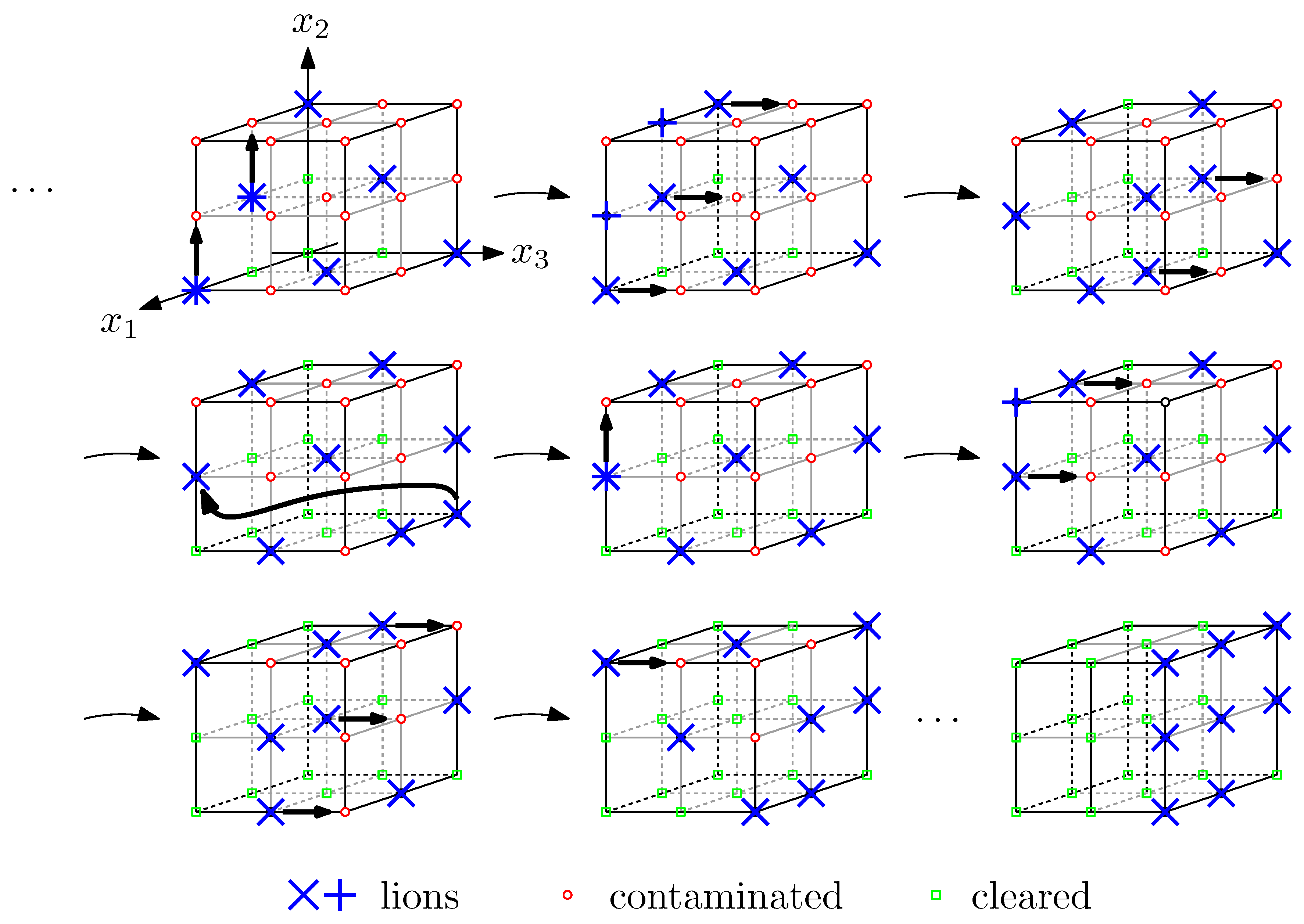
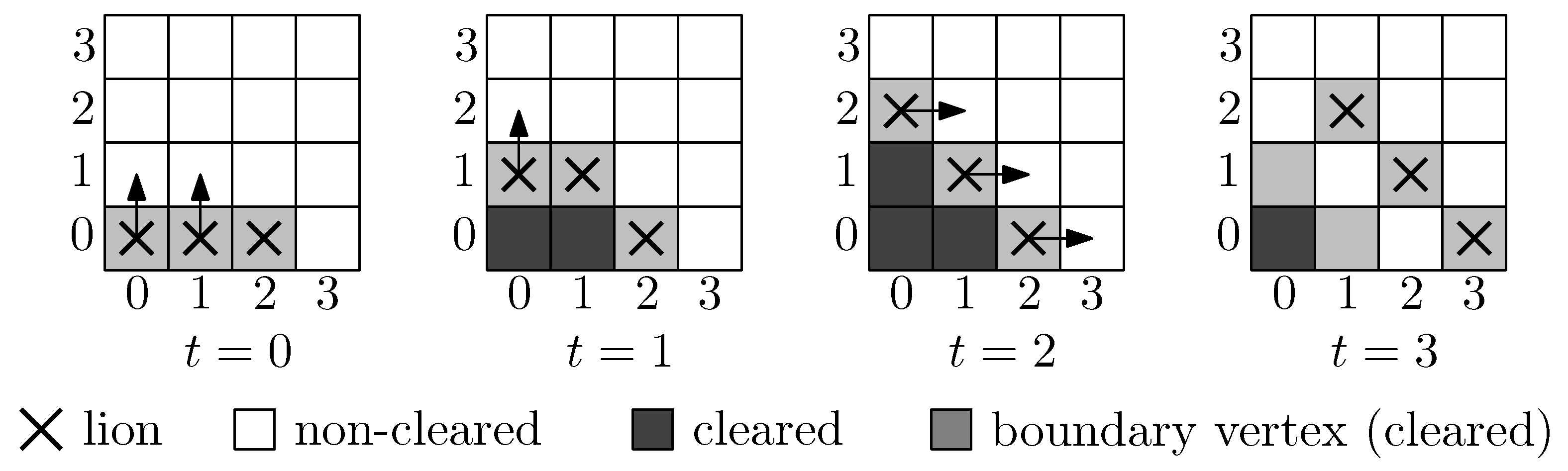
As mentioned in the introduction, one could conjecture $k_d\left(n\right)=n^{d-1}$. However, this does not even hold for $d=3$, see Figure 5. The movement can be done such that only one lion changes its location within each time step. All remaining lions can stay at their current positions and protect the cleared vertices. Even if the moving lion needs several steps to reach its destination, no problem arises.

Figure 5. Eight lions (rather than $n^{d-1}=9$) suffice to clear the $3\times 3\times 3$-grid. If two lions occupy the same vertex at the same time, this is indicated by two crosses of different orientation.

Figure 5. Eight lions (rather than $n^{d-1}=9$) suffice to clear the $3\times 3\times 3$-grid. If two lions occupy the same vertex at the same time, this is indicated by two crosses of different orientation.

For any grid vertex v, we denote the $L_1$-distance from v to the origin 0 as $\left|v\right|$.

The idea is to sweep the vertices layer by layer, where the r-th layer is the set of vertices of $L_1$-distance r to the origin. It is denoted by

$$L(r,n,d):=\{v\in {\left[n\right]}^d|\left|v\right|=r\}$$

For $r\le d(n-1)$ the value of $\left|L\right(r,n,d\left)\right|$ can be computed recursively by:

$$\begin{array}{c}\hfill \left|L(r,n,d)\right|=\sum _{i=max(r-n+1,0)}^{min(r,(d-1\left)\right(n-1\left)\right)}\left|L(i,n,d-1)\right|\end{array}$$

(3)

As start of the recursion, we can use $\left|L\right(r,n,1\left)\right|=1$ for $0\le r\le n-1$. To the best of our knowledge, no closed formula is known, but it is not difficult to prove the following Lemma.

Lemma 6. 

$\left|L\right(r,n,d\left)\right|$ is increasing in r for $0\le r\le \frac{d(n-1)}{2}$.

Proof. 

We use induction on d. For $d=1$, we have $\left|L\right(r,n,1\left)\right|=1$ for $0\le r\le \frac{n-1}{2}$, which is monotonously increasing.

Now, let us assume, we already showed for dimension d that $\left|L\right(r,n,d\left)\right|$ is increasing in r in the range of $0\le r\le \frac{d(n-1)}{2}$. Our task is to prove the monotonicity for dimension $d+1$.

Due to the symmetry $\left|L\right(r,n,d\left)\right|=\left|L\right(d(n-1)-r,n,d\left)\right|$, the induction hypothesis implies that $\left|L\right(r,n,d\left)\right|$ decreases monotonously in r in the range of $\frac{d(n-1)}{2}\le r\le d(n-1)$. The symmetry $\left|L\right(r,n,d\left)\right|=\left|L\right(d(n-1)-r,n,d\left)\right|$ holds, because all grid points with distance r from the origin have distance $d(n-1)-r$ from the grid point $(n-1,\dots ,n-1)$ and vice versa.

Clearly, $\left|L\right(r,n,d+1)$ is monotonously increasing for $0\le r\le n-1$. For the remaining range $n-1\le r\le \frac{(d+1)(n-1)}{2}-1$, we have $r-n+1\ge 0$ and $r+1\le d(n-1)$. Hence, formula (3) leads to

$$\begin{array}{ccc}\hfill \left|L\right(r+1,n,d+1\left)\right|-\left|L\right(r,n,d+1\left)\right|& =& \sum _{i=max(r-n+2,0)}^{min(r+1,d(n-1\left)\right)}\left|L(i,n,d)\right|\hfill \\ & -& \sum _{i=max(r-n+1,0)}^{min(r,d(n-1\left)\right)}\left|L(i,n,d)\right|\hfill \\ & =& \left|L\right(r+1,n,d\left)\right|-\left|L\right(r-n+1,n,d\left)\right|\hfill \\ & =:& x(r,n,d)\hfill \end{array}$$

We will prove the monotonicity of $\left|L\right(.,n,d+1\left)\right|$ by showing $x(r,n,d)\ge 0$.

If $r+1\le \frac{d(n-1)}{2}$, then $r-n+1$ as well as $r+1$ are in the increasing part of $s\mapsto \left|L\right(s,n,d\left)\right|$, hence $x(r,n,d)\ge 0$ and the monotonicity holds. For $\frac{d(n-1)}{2}<r+1\le \frac{(d+1)(n-1)}{2}$, the term $x(r,n,d)$ is monotonously decreasing in r, since $r+1$ is in the decreasing part of $s\mapsto \left|L\right(s,n,d\left)\right|$, while $r-n+1\le \frac{d(n-1)}{2}-\frac{n+1}{2}$ is still in the increasing part. But even if we chose $r=\lfloor \frac{(d+1)(n-1)}{2}\rfloor -1$, which is the maximum value for r we have to consider, we can still show $x(r,n,d)\ge 0$:

If d is odd or n is odd, we obtain $x(r,n,d)=|L(\frac{d(n-1)}{2}+\frac{n}{2}-\frac{1}{2},n,d)|-|L(\frac{d(n-1)}{2}-\frac{n}{2}-\frac{1}{2},n,d)|$, which equals $|L(\frac{d(n-1)}{2}-\frac{n}{2}+\frac{1}{2},n,d)|-|L(\frac{d(n-1)}{2}-\frac{n}{2}-\frac{1}{2},n,d)|\ge 0$ due to the symmetry. This shows that the monotonicity of $\left|L\right(.,n,d\left)\right|$ implies the monotonicity of $\left|L\right(.,n,d+1\left)\right|$ within the range needed for Lemma 6. Accordingly, if d is even and n is even, we obtain $x(r,n,d)=|L(\frac{d(n-1)}{2}+\frac{n}{2}-1,n,d)|-|L(\frac{d(n-1)}{2}-\frac{n}{2}-1,n,d)|\ge 0$. ☐

This proof shows that the middle layer, $L(\lfloor \frac{(n-1)d}{2}\rfloor ,n,d)$, is the biggest, which will be important for our estimates.

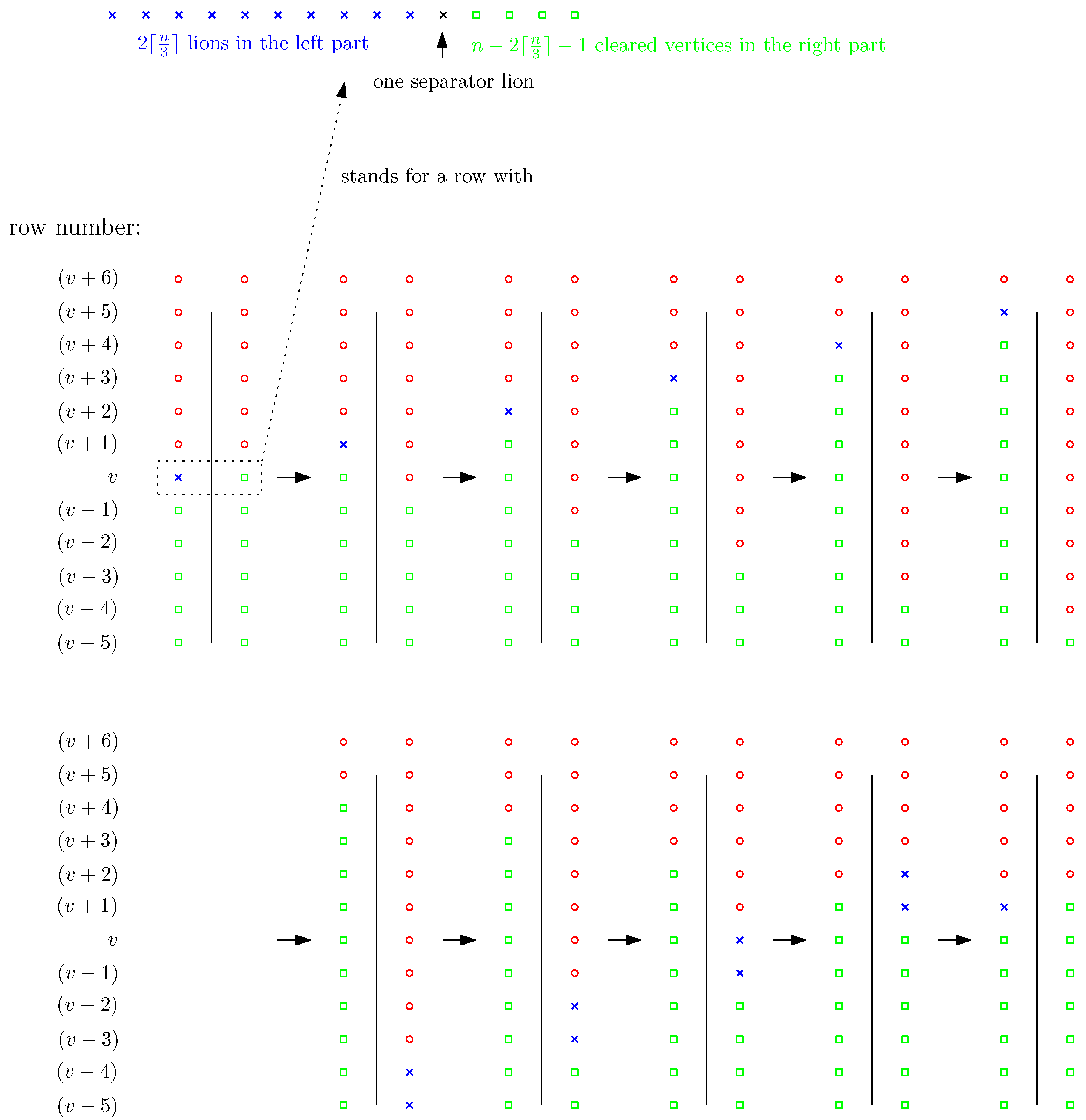
The strategy from Figure 5 can be generalized to grid graphs of arbitrary size and dimension. We sweep the grid $G_n^d$ layer after layer. No vertex of $L(r+1,n,d)$ is cleared before the last vertex of $L(r,n,d)$ has been.

Let us consider two consecutive layers $L(r,n,d)$ and $L(r+1,n,d)$, and let us assume that the former has been completely cleared, while the latter is still completely contaminated. Together they form a bipartite graph where every vertex has degree of at most d. How many lions are needed to clear $L(r+1,n,d)$ without recontamination?

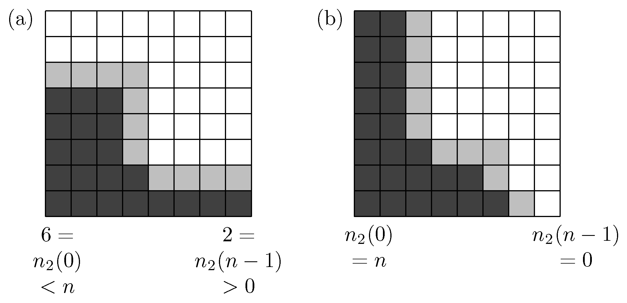
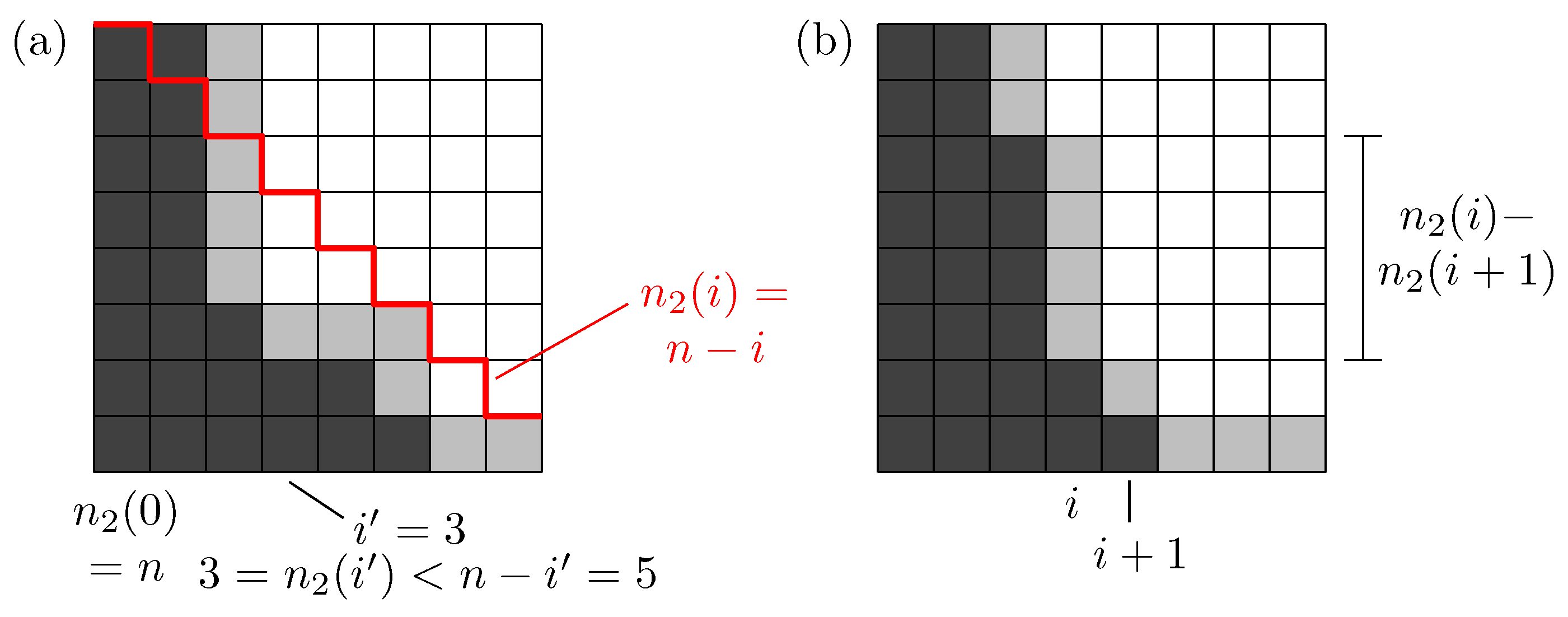
Lemma 7. 

Assume that the set $\{v\in {\left[n\right]}^d\mid |v|\le r\}$ is already cleared. At most $\left|L\right(r,n,d\left)\right|+\left|L\right(r+1,n,d-1\left)\right|$ lions are needed to clear $L(r+1,n,d)$ without recontamination, if $r+1\le (d-1)(n-1)$. In the remaining case, if $(d-1)(n-1)<r+1\le d(n-1)$, we need only $\left|L\right(r,n,d\left)\right|$ lions.

Proof. 

First, we notice that for every $(x_1,\dots ,x_d)\in L(r+1,n,d)$ with $x_d\ne 0$, $(x_1,\dots ,x_d-1)$ lies in $L(r,n,d)$. Furthermore, if there is an edge connecting $(x_1,\dots ,x_d)\in L(r,n,d)$ and $(y_1,\dots ,y_d)\in L(r+1,n,d)$, and $(y_1,\dots ,y_d)\ne (x_1,\dots ,x_d+1)$, then $y_d=x_d$.

Now, to clear $L(r+1,n,d)$ we proceed as follows: Initially, we place one lion at each vertex of $L(r,n,d)$. To do that, we obviously need $\left|L\right(r,n,d\left)\right|$ lions. If $r+1\le (d-1)(n-1)$, in addition, for every $y=(y_1,\dots ,y_d)\in L(r+1,n,d)$ with $y_d=0$, we place one lion on a vertex $x=(x_1,\dots ,x_d)\in L(r,n,d)$ with $x_d=0$, so that there exists an edge $(x,y)\in E_n^d$. For that, $\left|L\right(r+1,n,d-1\left)\right|$ lions are needed. The following algorithm shows that no further lion is necessary to clear $L(r+1,n,d)$.

In the first step, each one of the additional lions moves to its assigned vertex $y=(y_1,\dots ,y_{d-1},0)$. Now all vertices in $L(r+1,n,d)$ of this form have been cleared. Because every vertex of $L(r,n,d)$ is still occupied by a lion, no recontamination has occurred.

Next, we move lions from $L(r,n,d)$ to $L(r+1,n,d)$ without causing any recontamination. Beginning with $i=0$, we repeat the following action until i equals $n-1$ or r: Move every lion that is placed on a vertex of the form $(x_1,\dots ,x_{d-1},i)$ to $(x_1,\dots ,x_{d-1},i+1)$.

After this loop, every vertex of $L(r+1,n,d)$ is occupied, as follows from the remarks at the beginning of this proof. Moreover, no recontamination was possible during the loop, because every lion left his vertex via the only edge that led a contaminated vertex.

Note that in the case of $r+1>(d-1)(n-1)$ the layer $L(r+1,n,d)$ does not contain any vertex v with $v_d=0$. We can do the same as above with $\left|L\right(r,n,d\left)\right|$ lions. No additional lions are needed. ☐

As a consequence, we obtain the following upper bounds.

Lemma 8. 

$$\begin{array}{ccc}\hfill k_d\left(n\right)& \le & |L(\lfloor \frac{d(n-1)}{2}\rfloor ,n,d)|+|L(\lfloor \frac{d(n-1)}{2}\rfloor +1,n,d-1)|\hfill \\ & \le & 2|L(\lfloor \frac{d(n-1)}{2}\rfloor ,n,d)|\hfill \end{array}$$

Proof. 

From Lemma 7 we can conclude

$$\begin{array}{ccc}\hfill k_d\left(n\right)& \le & max\left(\underset{0\le r<(d-1)(n-1)}{max}\left|L(r,n,d)\right|+\left|L(r+1,n,d-1)\right|,\underset{(d-1)(n-1)\le r<d(n-1)}{max}\left|L(r,n,d)\right|\right)\hfill \\ & \le & \underset{0\le r<d(n-1)}{max}\left|L(r,n,d)\right|+\left|L(r+1,n,d-1)\right|\hfill \end{array}$$

The recursive formula for $\left|L\right(r,n,d\left)\right|$ implies

$$\left|L(r,n,d)\right|+\left|L(r+1,n,d-1)\right|\le \sum _{i=max(0,r-n+1)}^{r+1}\left|L(i,n,d-1)\right|$$

We want to establish that ${\sum }_{i=max(0,r-n+1)}^{r+1}\left|L(i,n,d-1)\right|$ obtains its maximum for $r=\lfloor \frac{d(n-1)}{2}\rfloor$. The above sum contains at most $n+1$ consecutive elements of the sequence:

$$\begin{array}{c}\hfill {\left(\left|L\right(i,n,d-1\left)\right|\right)}_{0\le i\le (d-1)(n-1)}\end{array}$$

By Lemma 6 and its proof, we know that this sequence is monotonously increasing for $i\le \frac{(d-1)(n-1)}{2}$, monotonously decreasing for $i\ge \frac{(d-1)(n-1)}{2}$ and symmetric with respect to $i=\frac{(d-1)(n-1)}{2}$. Hence, the sum is maximized if $n+1$ consecutive sequence indices are chosen as symmetrically as possible around $\frac{(d-1)(n-1)}{2}$.

If $n+1$ is odd and d is odd, a maximum sum arises if $r+1-\frac{n}{2}=\frac{(d-1)(n-1)}{2}$. If $n+1$ is odd and d is even, a maximum sum arises if $r+1-\frac{n}{2}=\frac{(d-1)(n-1)}{2}+\frac{1}{2}$. In the third case, if $n+1$ is even, a maximum sum is obtained for $r-\frac{n}{2}+\frac{1}{2}=\frac{(d-1)(n-1)}{2}$.

In all three cases, the sum ${\sum }_{i=max(0,r-n+1)}^{r+1}\left|L(i,n,d-1)\right|$ obtains its maximum for $r=\lfloor \frac{d(n-1)}{2}\rfloor$. This proves the first inequality of the Lemma. The second one is a simple but not very tight estimate. ☐

4.2. A lower bound

Now, that we found an upper bound on $k_d\left(n\right)$ in terms of the size of the middle layer, we want to prove that $L:=|L(\lfloor \frac{(n-1)d}{2}\rfloor ,n,d)|$ also determines a lower bound.

The proof is based on a result by Bollabás and Leader [4] which uses the following simplicial order on ${\left[n\right]}^d$. For every two vertices $v,w\in {\left[n\right]}^d$ we have

$$\begin{array}{ccc}\hfill v<w& :\iff & \left|v\right|<\left|w\right|\vee \hfill \\ & & \left(\left|v\right|=\left|w\right|\wedge \exists j\in \left[n\right]:\left(v_j>w_j\wedge \forall i<j:v_i=w_i\right)\right)\hfill \end{array}$$

Let $v^1:=0:=(0,\dots ,0)$, $v^2:=(1,0,\dots ,0)$, $v^3:=(0,1,0,\dots ,0)$, … denote the vertices in simplicial order. And for every $i\in \{1,\dots ,n^d\}$ let $A_i:=\{v^1,\dots ,v^i\}$ be the set of the first i vertices with respect to the simplicial order. Then, $|\partial A_i|$ denotes the number of boundary vertices of $A_i$.

With this notation we can formulate the following important kind of isoperimetric inequality.

Lemma 9. 

For every given size $m\in \{1,\dots ,n^d\}$ the set $A_m$ attains the minimum number of boundary vertices, i.e.

$$\forall C\subseteq {\left[n\right]}^d:\left|C\right|=m\Rightarrow \left|\partial C\right|\ge |\partial A_m|$$

Proof. 

For every $A\subseteq {\left[n\right]}^d$ and every $r\in \{1,\dots ,n(d-1\left)\right\}$ one defines the closed neighborhood of A as

$$\mathcal{N}\left(A\right):=\{v\in {\left[n\right]}^d|\exists w\in A:|v-w|\le 1\}$$

Then, Theorem 8 in [4] states that every $C\subseteq {\left[n\right]}^d$ of $m:=\left|C\right|$ vertices satisfies $\left|\mathcal{N}\left(C\right)\right|\ge |\mathcal{N}\left(A_m\right)|$. This can be translated into our Lemma 9 as follows:

$$\begin{array}{c}\hfill \left|\partial C\right|=|\mathcal{N}\left(\overline{C}\right)|-|\overline{C}|=|\mathcal{N}\left(\overline{C}\right)|-|\overline{A_m}|\ge |\mathcal{N}\left(\overline{A_m}\right)|-|\overline{A_m}|=|\partial A_m|\end{array}$$

☐

Now we can prove a lower bound in terms of the middle layer.

Lemma 10. 

$k_d\left(n\right)\ge \lfloor \frac{1}{6}L\rfloor$.

Proof. 

Let us consider the paths of $k_d\left(n\right)$ lions successfully cleaning the grid. By Lemma 1, the number of cleared vertices increases by at most $k_d\left(n\right)$ within each step. Consequently, there must be some moment t such that $\frac{n^d}{2}-k_d\left(n\right)\le \left|\mathcal{C}\left(t\right)\right|\le \frac{n^d}{2}$ and $\left|\mathcal{C}\right(t+1\left)\right|>\left|\mathcal{C}\right(t\left)\right|$. Thanks to Lemma 2, we obtain

$$k_d\left(n\right)\ge \frac{1}{2}\left|\partial \mathcal{C}\left(t\right)\right|.$$

Thus we have to lower bound the number of boundary vertices of a subset of the grid with size $\left|\mathcal{C}\right(t\left)\right|$. By Lemma 9, the fewest boundary vertices for such a set are obtained by the set $A_{\left|\mathcal{C}\right(t\left)\right|}$. Thus, $k_d\left(n\right)\ge \frac{1}{2}\left|\partial A_{\left|\mathcal{C}\right(t\left)\right|}\right|$.

Let us assume there exist $n,d$ such that $k_d\left(n\right)<\lfloor \frac{1}{6}L\rfloor$. Then both nodes $v^{\lceil \frac{n^d}{2}\rceil -k_d\left(n\right)}$ and $v^{\lfloor \frac{n^d}{2}\rfloor }$ are contained in the middle layer, $L(\lfloor \frac{(n-1)d}{2}\rfloor ,n,d)$. We want to estimate the number of boundary vertices of $A_{\left|\mathcal{C}\right(t\left)\right|}$ contained in the middle layer. Let us first consider the situation for the set $A_{\lfloor \frac{n^d}{2}\rfloor }$, which contains half the number of all grid vertices. If $(n-1)d$ is even, half of the vertices of the middle layer are contained in $A_{\lfloor \frac{n^d}{2}\rfloor }$. If $(n-1)d$ is odd, $A_{\lfloor \frac{n^d}{2}\rfloor }$ contains all vertices of the middle layer and no vertex of the neighboring layer with distance $\lceil \frac{(n-1)d}{2}\rceil$ from the origin. In both cases, there are at least $\lfloor \frac{1}{2}L\rfloor$ boundary vertices of $A_{\lfloor \frac{n^d}{2}\rfloor }$ in the middle layer of the grid.

Since $\frac{n^d}{2}-k_d\left(n\right)\le \left|\mathcal{C}\left(t\right)\right|\le \frac{n^d}{2}$ and $k_d\left(n\right)<\lfloor \frac{L}{6}\rfloor$, the sets $A_{\lfloor \frac{n^d}{2}\rfloor }$ and $A_{\left|\mathcal{C}\right(t\left)\right|}$ differ in at most $k_d\left(n\right)$ middle layer vertices. We conclude that $A_{\left|\mathcal{C}\right(t\left)\right|}$ contains at least $\lfloor \frac{1}{2}L\rfloor -k_d\left(n\right)$ boundary vertices in the middle layer. Hence,

$$k_d\left(n\right)\ge \frac{1}{2}\left|\partial A_{\left|\mathcal{C}\right(t\left)\right|}\right|\ge \frac{1}{2}⌊\frac{L}{2}⌋-\frac{1}{2}{k}_d\left(n\right)>\frac{1}{2}⌊\frac{L}{2}⌋-\frac{1}{2}⌊\frac{L}{6}⌋\ge ⌊\frac{L}{6}⌋$$

To verify the last inequality, we notice that the value of $\frac{1}{2}⌊\frac{L}{2}⌋-\frac{3}{2}⌊\frac{L}{6}⌋$ depends only on $Lmod6$, thus it is sufficient to check the cases $0\le L\le 5$. What we obtained is a contradiction to our assumption $k_d\left(n\right)<\lfloor \frac{L}{6}\rfloor$. ☐

4.3. An asymptotic estimate

We have given upper and lower bounds on $k_d\left(n\right)$ in terms of the size of the middle layer, thereby proving $k_d\left(n\right)\in \Theta (L(\lfloor \frac{(n-1)d}{2}\rfloor ,n,d)|)$. But how does this size grow? Unfortunately, we are not aware of a closed formula for $|L(\lfloor \frac{(n-1)d}{2}\rfloor ,n,d)|$ in general. But the following folklore result [14] describes an asymptotic estimate.

Lemma 11. 

$|L(\lfloor \frac{(n-1)d}{2}\rfloor ,n,d)|\in \Theta (\frac{n^{d-1}}{\sqrt{d}})$

Proof. 

Let us consider d independent and identically distributed random variables $X_1,\dots ,X_d$ each of which can take any integer value from 0 to $n-1$ with equal probability. Each $X_i$ has expectation $\frac{n-1}{2}$ and variance $\frac{n^2-1}{12}$. Therefore, the random variable $S_d^n:=X_1+\dots +X_d$ has expectation $\frac{d(n-1)}{2}$ and variance $\frac{d(n^2-1)}{12}$. By the central limit theorem, the distribution of $\frac{S_d^n-\frac{d(n-1)}{2}}{\sqrt{\frac{d(n^2-1)}{12}}}$ converges towards the standard normal distribution. This means, that the probability of the event $S_d^n=⌊\frac{d(n-1)}{2}⌋$ asymptotically behaves like $\frac{1}{\sqrt{2\pi }}{\int }_{-1/\left(2\sqrt{d(n^2-1)/12}\right)}^{1/\left(2\sqrt{d(n^2-1)/12}\right)}exp(-\frac{t^2}{2})dt$. For increasing n and/or d, the integration domain shrinks around 0, hence the integrand stays in an interval $[1-\epsilon ,1]$ where $\epsilon \searrow 0$. The probability lies in the interval $\left[(1-\epsilon )\sqrt{\frac{6}{\pi d(n^2-1)}},\sqrt{\frac{6}{\pi d(n^2-1)}}\right]$. Multiplying this by $n^d$, which is the number of all vertices in the grid, leads to the fact that the number of vertices in the middle layer asymptotically behaves like $\Theta (\frac{n^{d-1}}{\sqrt{d}})$. ☐

We can combine Lemmas 8, 10 and 11 to

Theorem 2. 

$k_d\left(n\right)\in \Theta \left(\right|L(\lfloor \frac{(n-1)d}{2}\rfloor ,n,d)\left|\right)=\Theta (\frac{n^{d-1}}{\sqrt{d}})$

5. Flying lions in the 2-dimensional grid

We are not aware of any strategy with fewer than n lions to clear the two-dimensional $n\times n$-grid. Indeed, we conjecture that n is the clearing number of the $n\times n$-grid. In this section, we will establish that fewer than n lions are sufficient, if the lions are able to fly.

To be more precise, we consider the problem variant where the movement of the lions is not restricted to the edges of the grid. If a lion moves from a grid vertex to an adjacent grid vertex, this still prevents the contamination from using the corresponding edge in the other direction. However, if a lion flies from a grid vertex to another vertex which is not adjacent in the grid, no edge is protected.

Our proof of Theorem 1 in Section 3. does not take any advantage of the fact that the movement of the lions is restricted to grid edges. This means, the lower bound of $\frac{n}{2}$ is still valid for the case of flying lions.

Our main result is that $\frac{n}{2}+O\left(\sqrt{n}\right)$ flying lions can clear the $n\times n$-grid. However, we start with showing the weaker result that $\frac{2}{3}n+O\left(1\right)$ lions are enough in order to illustrate the idea of our method in a simpler case.

For $h:=2\lceil \frac{n}{3}\rceil$, we denote the grid vertices with x-coordinate at most $h-1$ as the left part of the grid, while the vertices with x-coordinate at least $h+1$ are the right part. The vertices with x-coordinate equal to h are called separator vertices. Our strategy guarantees that the set of lions occupying separator vertices stays the same all the time. Lions belonging to this set are called separator lions.

We will describe a strategy enabling $h+11$ lions to clear one row of the grid after the other.

Suppose, we are given a situation where the 0th, 1st, …, v-th row of the grid are free of contamination, where $5\le v\le n-6$. The vertices $(0,v),(1,v),\dots ,(h-1,v)$ as well as the separator vertices $(h,v-5),(h,v-4),\dots ,(h,v+5)$ are occupied by the lions.

The movement of the lions is illustrated in Figure 6. The 11 lions located on the separator vertices keep their position until all of them move one row upwards when the complete $(v+1)$-th row and everything below is free of contamination. The first 5 steps are used to move the lions in the left part of the grid upwards. Afterwards, all lions from the left part fly to the right part, where they occupy all vertices of the $(v-5)$-th and $(v-4)$-th row. In the following 3 steps, the lions move upwards in the right part of the grid. Within each step, they gain two rows in the right part of the grid. For each such step, the upper lion in each column uses the grid edge to move one row upwards, while the lower lion flies to its new location three rows upwards. This kind of movement avoids any recontamination in the right part of the grid. Afterwards, all lions of the right part of the grid fly into the left part again, namely into the $(v+1)$-th row. What we obtained is the initial situation with $v+1$ instead of v. Or, to say it with other words: the lions gained one row.

Figure 6. Flying lions gain one row. The vertical black line segments partition the grid with ratio 2:1. The vertices corresponding to the black segments are occupied by lions, hence no contamination crosses them. Red circles are contaminated vertices, green boxes are cleared vertices and blue crosses are lions.

Figure 6. Flying lions gain one row. The vertical black line segments partition the grid with ratio 2:1. The vertices corresponding to the black segments are occupied by lions, hence no contamination crosses them. Red circles are contaminated vertices, green boxes are cleared vertices and blue crosses are lions.

Notice that, if $v<5$ or $v>n-6$, the situation is even better for the lions. Starting from the 0th row, they can consecutively clear one row after the other. After each gained row, all separator lions move one row upwards during the next time step. This happens simultaneously to the lions in the left part of the grid moving upwards. The total number of lions needed for this strategy is $h+11\in \frac{2}{3}n+O\left(1\right)$.

Lemma 12. 

$\frac{2}{3}n+O\left(1\right)$ flying lions can clear the $n\times n$-grid.

For a strategy in the above manner, the speed ratio between the upwards moving lions in one part of the grid and the downwards moving contamination in the other part does not have to be 2. If we save some lions, the speed advantage of the lions compared with the contamination gets smaller than 2, but the algorithm can still be performed. However, if we save too many lions, the problem is that the speed advantage gets so small that the number of separator lions dominates. It will turn out that a total number of $\frac{n}{2}+\Theta \left(\sqrt{n}\right)$ lions results in the best tradeoff between the number of lions operating in one part of the grid and the number of separator lions.

How does the speed advantage depend on the number of lions? Let us consider a grid with s columns and sufficiently many rows. As Figure 7 shows, $s+2$ lions can gain s rows in $s-1$ steps. This observation can be generalized to the following Lemma.

Lemma 13. 

Suppose, we are given a grid with s columns and sufficiently many rows. For $2\le r<s$, there is a strategy enabling $s+r$ lions to gain $\lceil \frac{s-r}{r-1}\rceil +2$ rows in $\lceil \frac{s-r}{r-1}\rceil +1$ steps.

Proof. 

The statement is restricted to a grid with s columns. No contamination from outside of these s columns has to be taken into account. The lions are using the strategy from Figure 7. We assume their start locations to be the s vertices of the vth row and the r leftmost vertices of the $(v+1)$-th row. Our strategy ensures that, at any time, there are only 2 rows containing lions. These rows are called active rows. Let w be the rightmost vertex occupied by a lion in the upper active row. All lions in the upper active row move one row upwards. Also, all lions in the lower active row which are right of w or directly under w move one row upwards. We still have $r-1$ lions left. These lions fly to vertices two rows upwards such that no gaps in this target row arises.

We repeat such moves until the upper active row is completely filled up with lions. Since each step increases the number of cleared vertices in the upper active row by $r-1$, exactly $\lceil \frac{s-r}{r-1}\rceil$ steps are needed. Afterwards, one more step is used to move all lions in the upper active row upwards, while the other lions fly three rows upwards to the leftmost positions. ☐

Now, we are ready to prove that $\frac{n}{2}+O\left(\sqrt{n}\right)$ flying lions are sufficient to clear the grid. This time, we choose the left and the right part of the grid of equal size.

The initial situation we consider is that the grid is cleared from the 0-th row up to the v-th row. We have $\frac{n}{2}$ lions located in the complete left part of the v-th row and $\lceil \sqrt{n}\rceil$ lions on the leftmost vertices of the $(v+1)$-th row. In terms of Lemma 13, we have $s=\frac{n}{2}$ and $r=\lceil \sqrt{n}\rceil$. For these values of s and r, it can be easily verified that $\lceil \frac{s-r}{r-1}\rceil +1\le \lceil \sqrt{n}\rceil$ for all $n\ge 2$.

Hence, by Lemma 13, we conclude that, if the lions in the left part of the grid move upwards for $3\lceil \sqrt{n}\rceil$ steps, they can gain $3\lceil \sqrt{n}\rceil +3$ rows there. During this time, the cleared area in the right part of the grid shrinks only by $3\lceil \sqrt{n}\rceil$ rows.

Now, the lions fly to their appropriate positions in the right part of the grid. Afterwards, $3\lceil \sqrt{n}\rceil +2$ rows remain gained in the left part—compared with the initial situation. In the right part, the lions occupy the complete $(v-3\lceil \sqrt{n}\rceil -1)$-th row and the $\lceil \sqrt{n}\rceil$ leftmost vertices of the $(v-3\lceil \sqrt{n}\rceil )$-th row.

In the following, the lions in the right part of the grid move upwards for $3\lceil \sqrt{n}\rceil$ steps. Comparing the situation afterwards with the initial situation, 2 rows are gained in both parts of the grid. Then, if the lions fly from right to left again, we have the initial situation with $v+1$ instead of v. Or, to say it with other words, the lions gained one row.

Figure 7. Speed advantage for the lions: they gain 6 rows in 5 steps.

Figure 7. Speed advantage for the lions: they gain 6 rows in 5 steps.

Besides the $\frac{n}{2}+\lceil \sqrt{n}\rceil$ lions operating either on the left or the right part of the grid, we also need the separator lions. The maximum vertical boundary they have to protect occurs when the lions are flying from left to right. A number of $6\lceil \sqrt{n}\rceil +3$ separator lions is sufficient. This means that the total number of all lions involved in this strategy is $\frac{n}{2}+7\lceil \sqrt{n}\rceil +3$.

Finally, we obtain:

Theorem 3. 

In the case of flying lions in the 2-dimensional grid, the clearing number is at least $\frac{n}{2}$ and at most $\frac{n}{2}+O\left(\sqrt{n}\right)$.