Content Sharing Graphs for Deduplication-Enabled Storage Systems

IBM Research at Almaden, 650 Harry Road, San Jose, CA 95120, USA
*
Author to whom correspondence should be addressed.
Algorithms 2012, 5(2), 236-260; https://doi.org/10.3390/a5020236
Submission received: 30 December 2011
/
Revised: 28 March 2012
/
Accepted: 29 March 2012
/
Published: 10 April 2012
(This article belongs to the Special Issue Data Compression, Communication and Processing)
Abstract
:Deduplication in storage systems has gained momentum recently for its capability in reducing data footprint. However, deduplication introduces challenges to storage management as storage objects (e.g., files) are no longer independent from each other due to content sharing between these storage objects. In this paper, we present a graph-based framework to address the challenges of storage management due to deduplication. Specifically, we model content sharing among storage objects by content sharing graphs (CSG), and apply graph-based algorithms to two real-world storage management use cases for deduplication-enabled storage systems. First, a quasi-linear algorithm was developed to partition deduplication domains with a minimal amount of deduplication loss (i.e., data replicated across partitioned domains) in commercial deduplication-enabled storage systems, whereas in general the partitioning problem is NP-complete. For a real-world trace of 3 TB data with 978 GB of removable duplicates, the proposed algorithm can partition the data into 15 balanced partitions with only 54 GB of deduplication loss, that is, a 5% deduplication loss. Second, a quick and accurate method to query the deduplicated size for a subset of objects in deduplicated storage systems was developed. For the same trace of 3 TB data, the optimized graph-based algorithm can complete the query in 2.6 s, which is less than 1% of that of the traditional algorithm based on the deduplication metadata.
1. Introduction
Motivated by the current data explosion, data reduction methods like deduplication and compression have become popular features increasingly supported in primary storage systems. The two techniques have interesting but contrasting properties—compression has a “local" scope (file, block, object) while deduplication has a global one. Although data reduction methods can save storage space for storage systems, they introduce new technical challenges to storage management, which is especially true for deduplication. Compression does not present great challenges to storage management as storage objects are not correlated with each other after data compression. However, for deduplication, storage objects (e.g., files) share data content among them in deduplication-enabled storage systems. Storage management tasks can no longer consider storage objects as independent. Traditionally, storage management systems assume there is no data sharing between storage objects, and therefore individual storage objects can be managed independently without affecting others. However, when storage objects share content with each other, they cannot be managed independently because management decisions on one file may affect another file. For example, in a traditional tiering storage system, individual old files can be migrated to a “colder” tier (e.g., from disks to tapes) without affecting other files. However, in a deduplicated tiering storage system, old files may share content with other files that are not necessarily old, so the migration of a candidate file needs to consider other files that share content with the candidate file, which can complicate the storage management tasks.
State-of-the-art deduplication-enabled storage systems [1,2,3,4,5,6] have not exploited the sharing among deduplicated set of files for the file management tasks. The file-to-chunk mappings are either kept internally as part of the per-file metadata [1,2,3,4] or externally as database tables [5,6]. To the best of our knowledge, this paper is the first in the open literature to leverage the deduplication metadata (the file-to-chunk mappings), to adapt them to graphs, and to explore graph-based algorithms to solve real-world file management problems on deduplication-enabled storage systems.
The key contribution of this paper is the introduction and showcase of the concept of a content sharing graph as a primitive to solve problems of storage management in deduplicated storage systems. Our graph structures illustrate the sharing of content between storage objects (e.g., files). The power of content sharing graphs lies in the fact that they reveal the hidden connectivity of individual storage objects, and enable graph-based algorithms to exploit the content sharing among storage objects. For example, in deduplicated storage systems, it is interesting to find out how many files share content with others; or what is the storage footprint of a set of deduplicated files.
Thus, by modeling content sharing as graphs, we can leverage existing graph research results to efficiently solve practical problems in the management of deduplicated storage systems. Among other management problems, in this paper, we solve two storage management problems using graph-based algorithms: (1) to partition a deduplication domain into sub-domains with minimal deduplication loss; and (2) to quickly find out the deduplicated size of a user-defined subset of files.
The rest of the paper is organized as follows. Section 2 defines content sharing graphs (referred to as CSGs) and presents two graph models to represent the same set of files in deduplicated storage systems. Section 3 provides two real-world problems that can be efficiently solved with graph-based algorithms, and a trace-driven analysis of these graph-based algorithms. Section 4 discusses the two proposed graph models. Section 5 presents related work in the field of storage management on deduplicated storage systems. Finally, Section 6 presents a summary of our results and concludes the paper.
2. Content Sharing Graphs
This section introduces content sharing graphs and defines key concepts associated with these structures with the aid of an example wherever necessary. In particular, we propose two graph models to represent the content sharing for the same set of storage objects in a deduplicated storage system.
2.1. Sparse Content Sharing Graph (SCSG)
SCSGgraphs are graph structures where vertices represent storage objects (files, blocks, volumes, etc.) and edges represent content shared between the connected vertices. To have a sparse and scalable graph, we require to use a minimum number of edges to represent sharing of the same content between files, that is, if the same chunk or group of chunks is shared by n files (vertices) we use edges. We illustrate below the construction of such graphs. Our primary use of these graphs was in analysis and visualization of deduplication content distribution in storage systems.
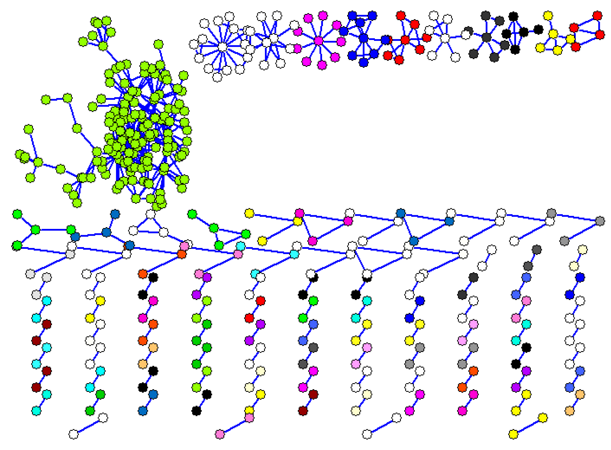
Figure 1 shows such an SCSGgraph representing the files (vertices) and the shared content (edges), for a folder on a Windows XP laptop.
Identical files (full file duplicates) are represented only once and singleton files (files that do not share any chunks with other files) are not represented in the graph. From a total of 8940 files in the folder, removing the singletons and file duplicates we were left with only 432 files (vertices shown in Figure 1) that share some content so are connected by edges. A component in the graph is a maximal subset of the vertices such that there is a path from every vertex in the subset to every other. The graph in Figure 1 has 103 components, most of them being small (two or three vertices), but there is a large component where the vertices are densely connected. The total number of edges connecting a vertex with its neighbors is the degree of the vertex.
To illustrate the construction of content sharing graphs we use a smaller folder (directory) on Windows XP consisting of 19 files (file IDs 1 to 19) with the content shown in Table 1. The file sizes vary between 20 and 60 bytes and they were created purposely to share content between themselves. To determine the content sharing between the files in a folder (or an entire file system) we first collect a “trace” by running a “file scanner” program that traverses each file of the folder (file system). The trace contains for each file a sequence of SHA1 content hashes, one hash for each chunk of the file. We use fixed chunk sizes, and for this example the chunk size is 4 bytes (for example, file #1 in Table 1 has 15 chunks and file #11 has 6 chunks, the last chunk in these files has the same content: “L111”). Note that in real applications the chunk sizes are much larger: 4 KB, 8 KB or larger.
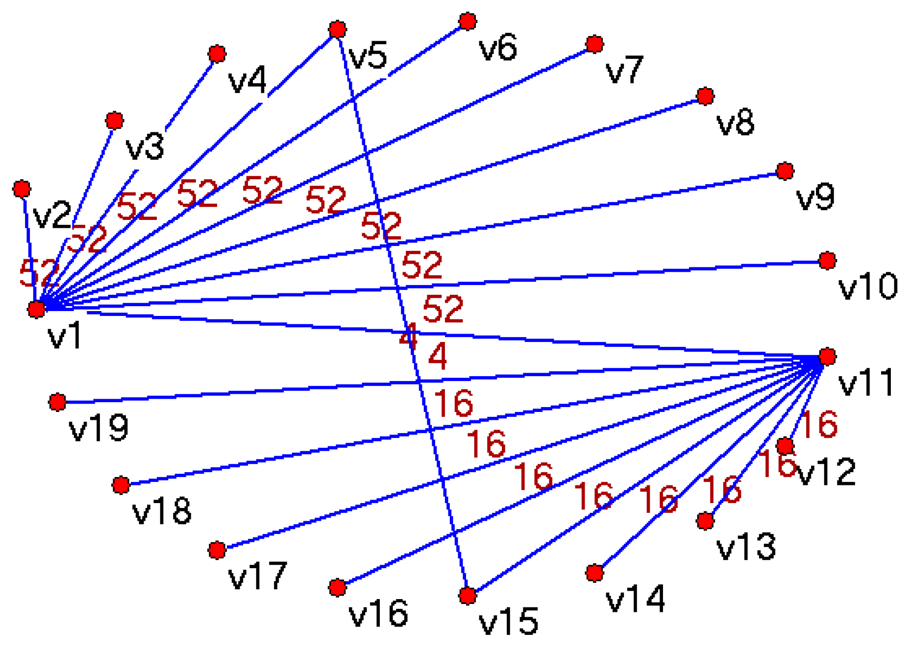
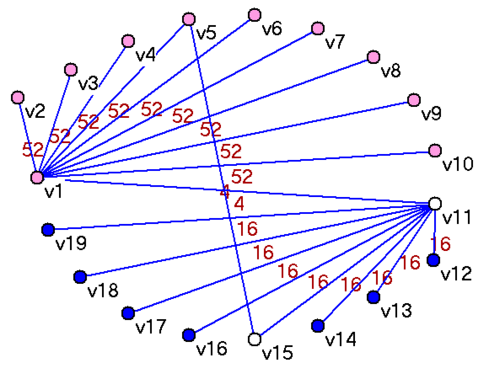
Given the 19 files with the content shown in Table 1 we can build an SCSGgraph as follows: each file is represented by a vertex, so we have {} vertices in our graph. Edges represent sharing of content between vertices and to have a minimum number of edges in the graph, we represent the shared content only once. Each edge has a weight representing the number of bytes shared by connected vertices. Representing the shared content only once provides another important property of the SCSGgraphs: the deduplicated size of the folder (file system) is simply the sum of vertex (raw file) sizes minus the sum of connecting edge weights. In Table 1 we see that file #1 to file #10 share chunks 2 to 14 (that is 13 chunks × 4 bytes = 52 bytes), and file #11 to file #19 share chunks 2 to 5 (20 bytes). One way to build an SCSGgraph with vertices {} is to connect with each vertex to by edges of weight 52 bytes, then to connect with each vertex to by edges of weight 20 bytes and finally to make explicit the sharing of the “brown” (last chunks in files #1 and #11) and “yellow” chunks (last chunks in files #5 and #15) by edges of weight 4 bytes. We get the SCSGgraph shown in Figure 2. We name this connection topology a STAR because from the n vertices sharing the same content we selected one (center of the star) to be connected with each other. The SCSGgraph for a folder on a Windows XP laptop shown in Figure 1 uses the STAR connection topology.
An alternative connection topology of an SCSGgraph for the set of 19 files in Table 1 is shown in Figure 3, where the n nodes sharing the same content are connected in a linked list fashion. We name this a CHAIN topology.
These connection topologies are just two somewhat extreme examples of SCSGgraphs. Any combination of them satisfies our definition of a SCSGgraph. The deduplicated size of the 19 files in Table 1 is the sum of the file sizes minus the sum of edge weights (in either one of the SCSGgraphs above), that is bytes.
2.2. Detailed Content Sharing Graph (DCSG)
Some applications need more detailed, chunk-level content sharing information for a set of deduplicated files. An example of such applications is the size computation for a subset of files in a deduplicated storage system (described in Section 3.3). For this reason, we introduce the DCSGgraph where there are two types of vertices: file vertices and sub-file vertices. File vertices represent files sharing content with each other (as in SCSGgraphs). A sub-file vertex represents a sharing unit among files, it can be a chunk or a range of adjacent chunks. In the following discussions, if not otherwise specified, we take individual chunks as default sub-file vertices for its simplicity, and we name these vertices chunk vertices. All edges in a DCSGare between file vertices and sub-file vertices. For this reason, DCSGgraphs are bi-partite graphs.
To build up a DCSGgraph one first needs to assign identifiers for unique chunks, where the identifer can be the hash value of the chunk or part of the hash. Next, one can get all edges associated with each file vertex or sub-file vertex by scanning the “deduplication metadata” that for each file has its attributes and the sequence of chunk hashes. Note that the edges do not have any associated properties (e.g., weights). All file-level attributes (e.g., file size, file modification time) are stored in the file vertices, and all chunk-level attributes (e.g., chunk size) are stored in the chunk vertices.
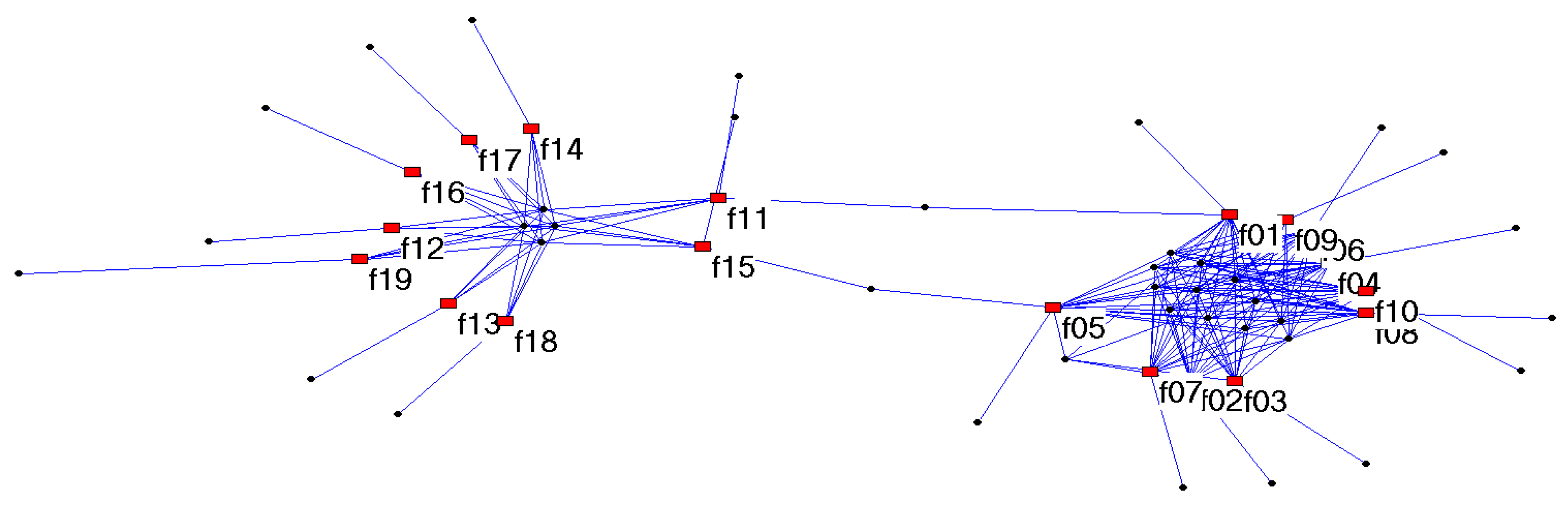
Figure 4 shows the DCSGgraph created from the small example, whose data is shown in Table 1. The rectangle vertices represent files, and ellipse vertices represent chunks. File identifers () are marked in the graph, but the chunk vertices are not marked. Each chunk vertex represents a chunk in the storage system, and its degree reflects how many times it has been referred to in the storage system. For example, chunk vertices with degree 1 belong exclusively to 1 file, while chunk vertices with degree more than one are shared by some files. The degree of a file vertex represents how many chunks belong to the particular file. Note that multiple edges between the same pair of file vertices and chunk vertices reflect the intra-file duplicates.
Because DCSGgraphs model the detailed sharing between files, they have a wide range of applications. While deduplication is about a set of files, individual files do not have a complete view regarding the deduplication information. When the set of files needs to be decomposed into smaller pieces or needs to be extended, individual files in the new set need to re-compute the deduplication information based on their chunks. For this reason, DCSGgraphs are important for these applications.
3. Use Cases of Graphs
3.1. Data Sets
We evaluate our algorithms using two real workload traces taken from a commercial archival/backup solution. Deduplication in the traces is based on variable size chunking that used SHA1 to produce chunk fingerprints. Table 2 shows the characteristics of the workloads, where WL1 and WL2 represent workload trace 1 and 2, respectively; we sometimes refer to them as “deduplication metadata”. In row 3, “Removable Duplicates" indicates the amount of duplicate chunks that are matches of unique chunks. In other words, a chunk with multiple appearances will be retained only once, other occurrences are removable duplicates. In row 4, “Deduplication Ratio" means the ratio of the amount of unique chunks over the amount of raw data.
3.2. Deduplication Domain Partitioning
Motivation
In deduplication-enabled storage servers, there are cases when some subsets of the entire deduplicated set of files need to be transferred to different servers or storage tiers, in deduplicated form, to provide scalability and load balance. One concrete case is in commercial backup/archival servers that deduplicate data on disk to save space and at some intervals (weekly, monthly) the deduplicated data need to be transferred to tapes for off line (or even off site) storage. There are a couple of constraints to be satisfied when storing deduplicated files on tapes. The first is to store all the (unique) chunks needed to reconstruct a file on the same tape (i.e., chunks of one file are not spread across many tapes). This will minimize the number of tape mounts needed when reading files from tape, and simplify the bookkeeping and transportation, especially when tapes are kept off-site. The second is to maintain the deduplication ratio close to that on disk (the original deduplication domain) when we place subsets of files on tapes. For this, each subset of files that are placed on the same tape should share most (all) of the chunks between themselves; any chunk shared with other subset going on a different tape needs to be replicated on both tapes. In this concrete case, the disk represents the original deduplication domain and tapes represent partitions of the disk domain into smaller, independent deduplication domains. These two constraints apply to many situations of deduplication domain partitioning. Thirdly, the sizes of the resulting partitions are roughly equal as default. But we usually relax this constraint in favor of first minimizing the deduplication loss due to partitioning. In another word, this constraint is optional.
Partitioning Algorithm
To solve the deduplication domain partitioning problem we employ an SCSGgraph model, introduced in Section 2.1, to represent the deduplication domain (original set of files in deduplicated form), and to partition this graph into subgraphs that represent subsets of files in deduplicated form, with minimal loss in overall deduplication ratio and without splitting files across partitions (each file, all its chunks, should fit in only one partition). Minimizing the deduplication loss for our SCSGgraph model means minimizing the total edge “cuts” (sum of edge weights between subgraphs). Remember that in SCSGgraphs, edge weights represent the number of bytes (sum of chunk sizes) shared by the two vertices (files) connected by the edge, so if these end vertices are in different partitions, the shared chunks have to be replicated (stored in each partition). As it is well known, the graph partitioning is an NP-complete problem [7]. We want to find a fast algorithm that exploits the characteristics of the content sharing SCSGgraphs for real workloads, and provide a good approximate solution to our deduplication domain partitioning.
Figure 1 shows the type of content sharing graphs we usually get. Indeed, representing our workloads (described in Section 3.1) by SCSGgraphs, we obtain a large number of small components (containing only few files each), and one or a few large components. Therefore, the first step of the partitioning algorithm is finding the components in the graph, which can be done in linear time with the size of the graph (number of edges) by a Breadth First Search (BFS) graph traversal. Generally, we obtain many small components, as in Figure 1, where the SCSGgraph consists of 103 distinct components, all relatively small with one exception. If each component size (sum of vertex sizes minus connecting edge weights) can fit in a partition (tape in the concrete case), then a greedy heuristic for the bin packing problem (like sorting the components in decreasing order of size and storing the components in this order in each partition) solves our partitioning.
However, if some component size is larger than the available space in any partition, then further partitioning of that component is needed. For this we are going to use an important concept, that of a k-core, introduced by social networks researchers [8,9]. A k-core of a graph is a maximal subgraph in which each vertex is adjacent to at least k other vertices (within the subgraph); therefore all the vertices within the k-core have a degree ≥k. We use an extension of the k-core concept where each edge contributes its weight (an integer number of bytes ≥1) to the computation of “degree”. The k-cores are nested (like the Russian dolls) one in the other, the highest into the lowest, each vertex having a “coreness” number that is the highest k in the k-cores it belongs to (note that all vertices in a connected component belong to the 1-core, just by being connected). The coreness for all vertices can be computed very fast, in almost linear time in the number of vertices, in one graph traversal with local computation of vertex degrees. In addition to the coreness numbers, in another BFS traversal, we compute the estimated deduplicated size of each k-core, that is, the sum of vertex sizes minus the sum of edge sizes inside each k-core. We use this estimated deduplication size to decide what k-core to extract in an optimal partitioning plan.
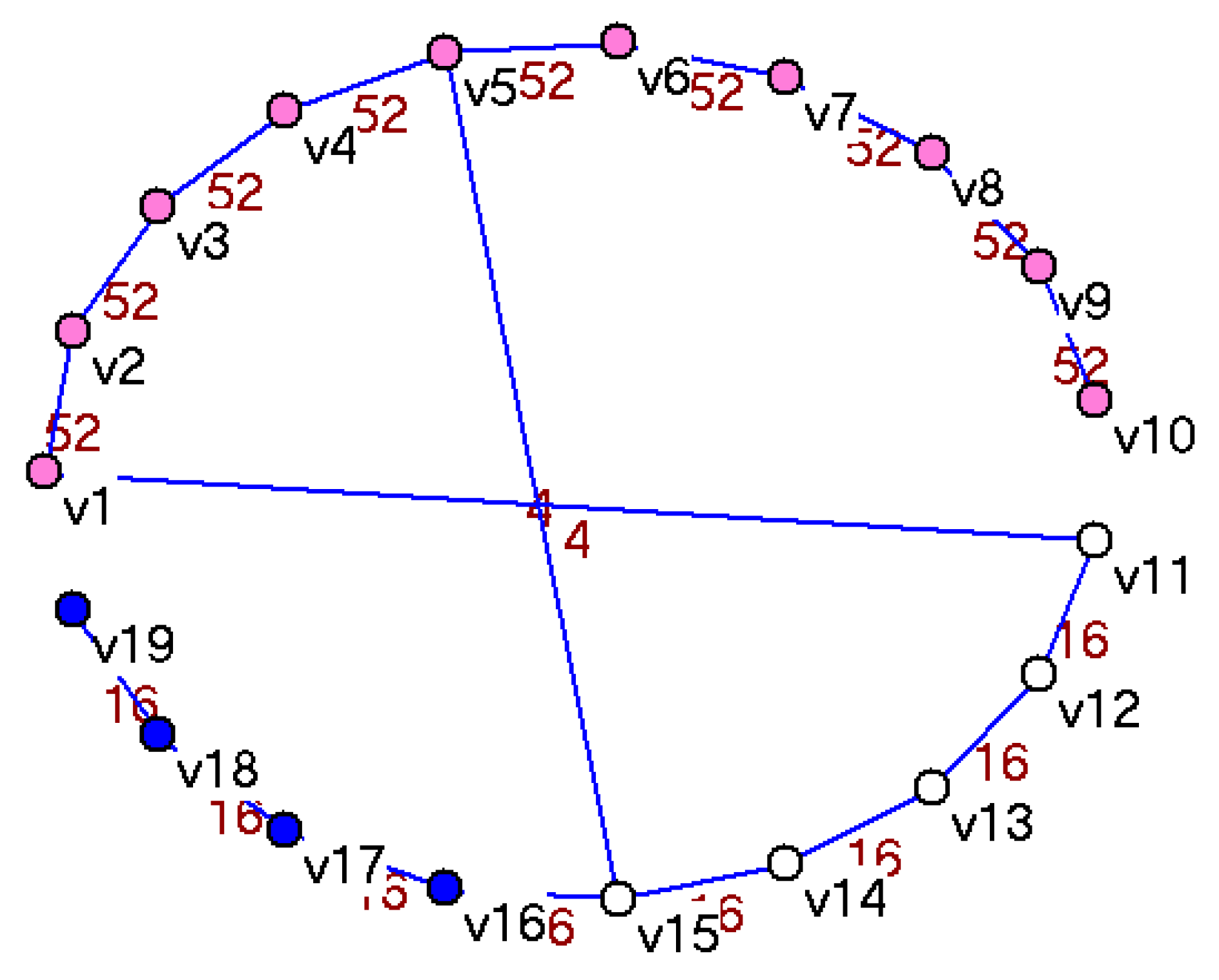
To illustrate the k-core decomposition and k-core size computation let us take as example the 19 files described in Table 1 and say that we want to partition them into two partitions (subsets) in such a way that (1) we have a minimal loss in deduplication (due to replication of chunks shared across partitions), (2) each file (all its chunks) belongs to only one partition and (3) the partitions have sizes relatively close to each other. We represent the files by an SCSGgraph, as in Figure 3 or Figure 2 and compute the k-cores decomposition for each representation. The k-core values represent the minimum bytes shared between any vertices belonging to the core. Figure 5 shows the three core decomposition for the CHAIN topology and Figure 6 shows the cores for the STAR connection topology of the SCSGgraph. Table 3 shows the vertices contained in each of the three cores for the set of 19 files in Table 1. Note the “nesting” of the cores—the top core with 10 vertices (with a minimum sharing 52 bytes) is included in middle core (with a minimum sharing 20 bytes) that in turn is included in the lower core (with a minimum sharing 16 bytes) that contains all the vertices (19 files).
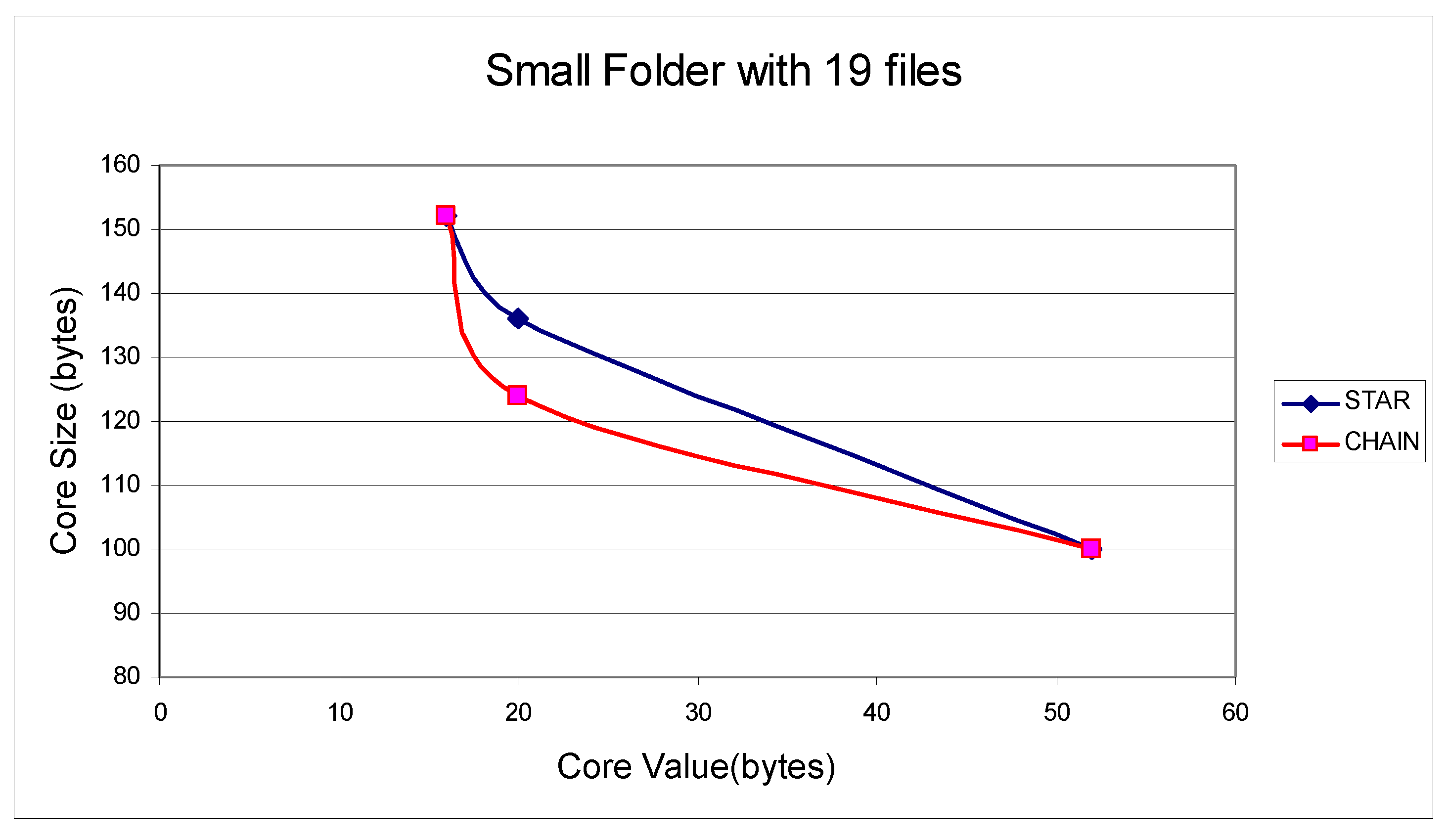
To help decide what k-core to extract, i.e., where to cut, we also estimate the k-core (deduplicated) sizes. In Figure 7 we show the deduplicated sizes for each core for both connection topologies.
The best place to partition the SCSGgraph for this small example is by extracting the k-core “52” with deduplicated size of 100 bytes as one partition and the remaining part of the graph (the “periphery”) as the second partition of 60 bytes as the deduplicated size. The “cut” size (partitioning cost) is 8 bytes due to cutting the 2 edges (i.e., storing the shared bytes in both partitions) between core “52” and “20” with weights (sharing) 4 bytes each. This is true for both connection topologies CHAIN and STAR.
In realistic cases, as shown in the next section, there are thousands of k-cores in the graph, all nested into each others from top, the densest connected, to the sparsest connected toward the periphery. As this small graph example shows, it is a good heuristic to “cut” outside the densest k-cores if possible. The edge weights are high inside the densest k-cores, so cutting in the middle of top k-cores is expensive. The densest k-cores for the real workloads are usually small in size, as will be shown next, so they do not need to be cut.
Results for the Real Workloads WL1 and WL2
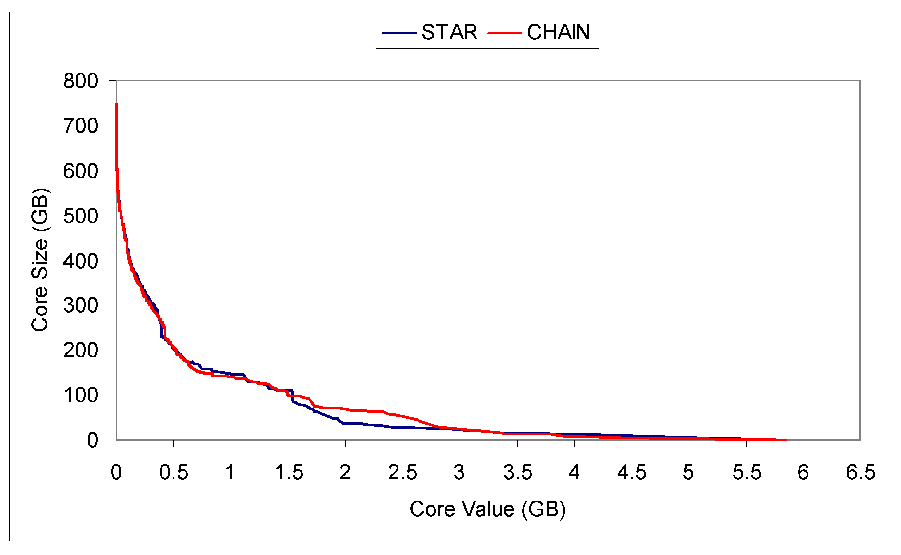
Table 4 shows the characteristics of the SCSGgraphs generated from the traces WL1 and WL2. Figure 8 shows the deduplicated (estimated from the graph) core size for each core, for both connection topologies, for workload WL1 (this is similar to Figure 7 for the small set of 19 files). Only the largest component of (deduplicated) size 746 GB (as shown in Table 4) is partitioned with k-cores. As all the vertices are contained in k-core 0, the size of k-core 0 is 746 GB. As can be seen in Figure 8 the sizes of the top k-cores (with minimum sharing between any pair of vertices over 3 GB) are very small.
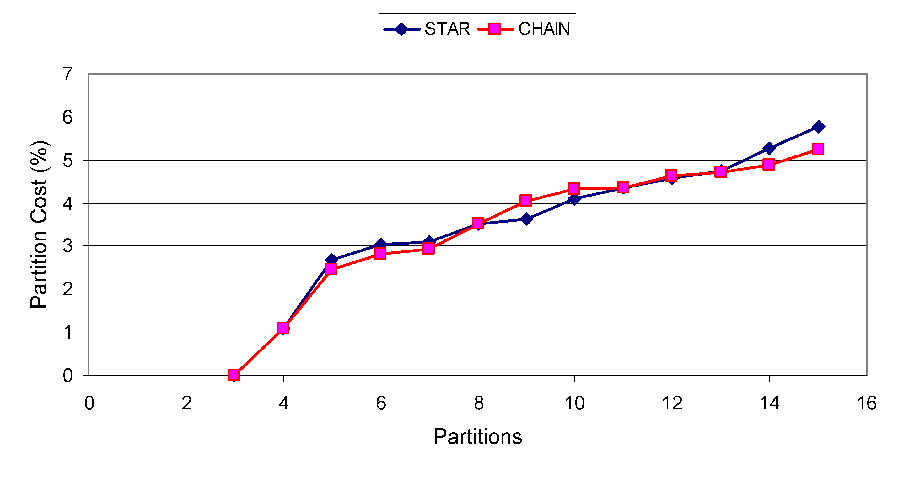
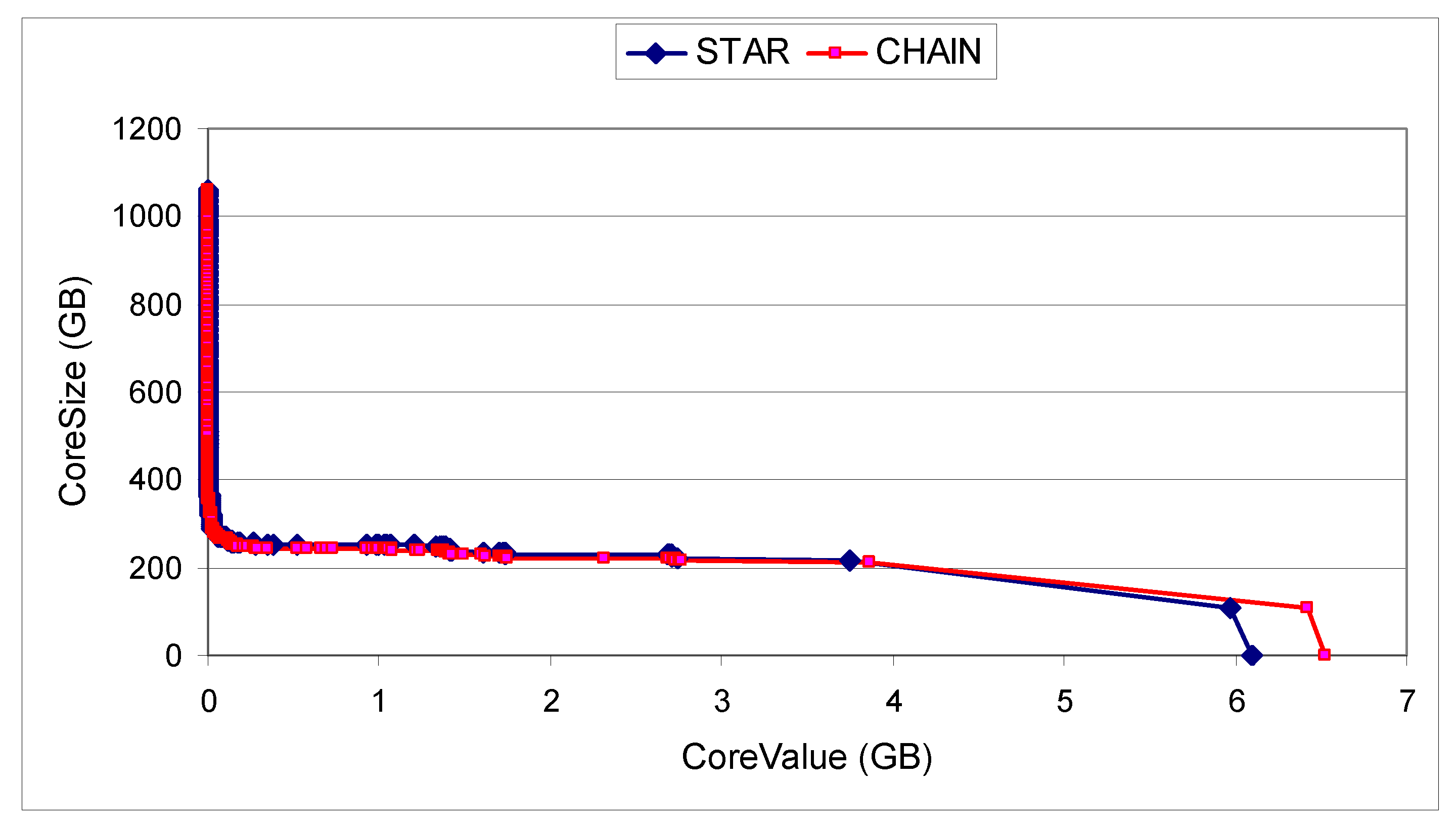
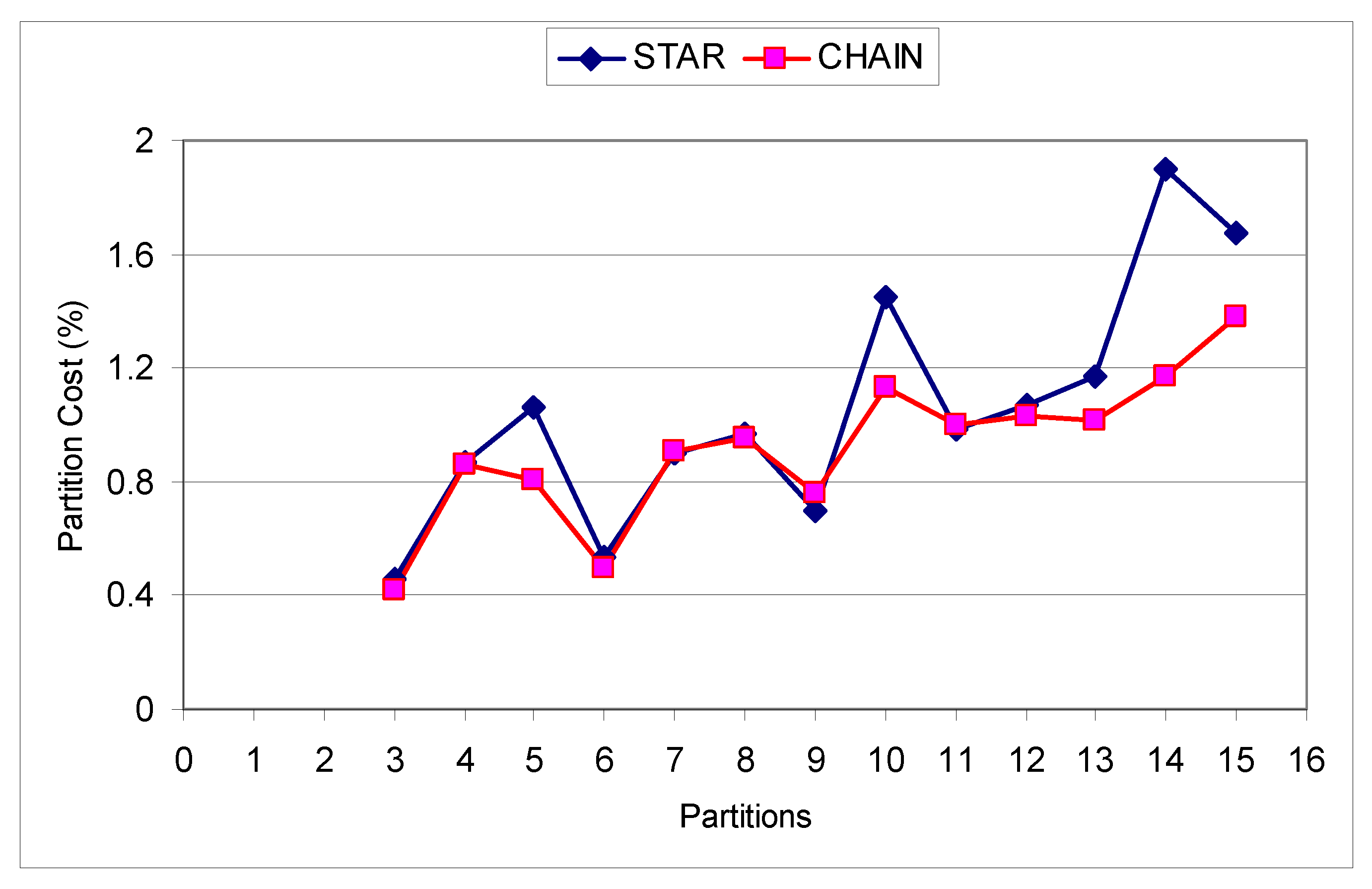
Figure 9 shows how the deduplication loss varies with the number of equal partitions we want to split the WL1 SCSGgraph into. To quantify the deduplication loss we define partitioning cost as the amount of replicated data across partitions (due to the edge cuts in the partitioning process) divided by the total amount of removable duplicate data (before partitioning). As can be seen, the smaller the partition sizes are (the more partitions are), the higher the partition cost is. This is because for smaller partitions the cuts are in the denser k-cores. However, even when we partition into 13 partitions, the partitioning cost is still less than 5%. Note that there is not much difference if the SCSGgraph uses the CHAIN connection topology or STAR. Figure 10 shows the (deduplicated) core size for each core, for both connection topologies, for workload WL2. Only the largest component of (deduplicated) size 1060 GB (as shown in Table 4) is partitioned with k-cores. This is somewhat different than the corresponding plot for WL1 in Figure 8. Digging deeper to see why there is such a rapid increase in the core sizes for small core values (close to 0), we found that for core value less than 1.4 MB (close to 0 in terms of GB), there are 25,822 files, their total raw size of 660,581,983,796 bytes, and their deduplicated size is 654,366,144,648 bytes. In other words, these files share very little (less than 1%) between themselves (the deduplicated size is almost equal with raw size), so they are almost singleton (share nothing) files. On the other hand, the horizontal part of the graph (the plateau) at about 220 GB is due to almost full file duplicates (files that share significant amount, say 99% of content between themselves). So this workload WL2 is composed either from files that share almost nothing or files that share almost everything with others. There is no gradual (smooth) distribution of sharing. Figure 11 shows how the deduplication loss varies with the number of equal partitions we want to split the WL2 SCSGgraph into. Even when we divide into 15 partitions, the partitioning cost is still less than 2%. There is a slightly better partitioning cost if the SCSGgraph uses the CHAIN connection topology than STAR.
3.3. Size Calculation for Deduplicated File Sets
Motivation
Administrators of modern large-scale storage systems are interested to know the space consumption of a subset of files, where the subset of interest is defined by administrators. For example, “what applications and users use the most of space”, “how much space do pdf files consume”, etc. Since the subset of files are defined at the query time, the size of the user-defined subset has to be computed on the fly from the metadata. We denote such queries as on-demand sizequeries. The on-demand nature of such queries poses a significant challenge to traditional metadata management systems and methods. As proposed by Leung et al. [10] and Hua et al. [11], a new set of metadata structures and related methods are required to efficiently answer on-demand queries (including on-demand sizequeries) for a large-scale storage system. The output of such queries is a subset of files that meet the query criteria.
Deduplication in storage systems further complicates the problem because the size of a subset of files is not simply the sum of the sizes of all files in the subset, i.e., even after we get the list of files that meet the query criteria, we cannot have a sum of the selected file sizes as these files may share content with each other. In this paper, we focus our discussion on how to calculate the accurate size of such a deduplicated set of files after we get the list of files from file subset queries.
The state-of-the-art practice is to query the deduplication metadata containing the signatures of either file of sub-file chunks, which is not scalable with the storage system size. To compute the size of a deduplicated subset of files, it is inevitable to deduplicate the subset of files by scanning all related file chunks and querying the deduplication metadata accordingly. We propose a relatively small metadata layer that is extracted from the raw deduplication metadata, to help efficiently answer on-demand sizequeries in a deduplicated storage system.
The DCSGgraph is a good candidate for such an efficient metadata layer for two reasons. First, the DCSGgraph accurately models the sharing between files for either a full set of files or for a subset of files. Second, the DCSGgraph has the potential to reduce its memory footprint by aggregating adjacent shared chunks. Experimental results show that aggregating adjacent shared chunks can effectively reduce the memory footprint of the DCSGgraph.
In the following discussion, we first describe how the state-of-the-art practice answers on-demand sizequeries using only the raw deduplication metadata in a database. We name this approach the “naive” algorithm. We then describe a straightforward algorithm based on DCSGgraphs, which we name the “graph” algorithm, and a refined, scalable algorithm by aggregating adjacent shared chunks, which we name the “optimized graph” algorithm or GraphOpt. Finally we present the experimental results of comparing these three algorithms with the data sets described in Section 3.1.
The Naive Algorithm
Without graphs, the naive algorithm answers on-demand sizequeries by running SQL queries against the database containing deduplication metadata. In a deduplicated storage system, there is one table that comprises the deduplication metadata: the chunk information table (denoted as ). Among other fields, the query-related fields in are , where is the unique file identifier, is the length of the chunk, and is the hash value of the chunk for deduplication (e.g., 20-byte MD5 hash value).
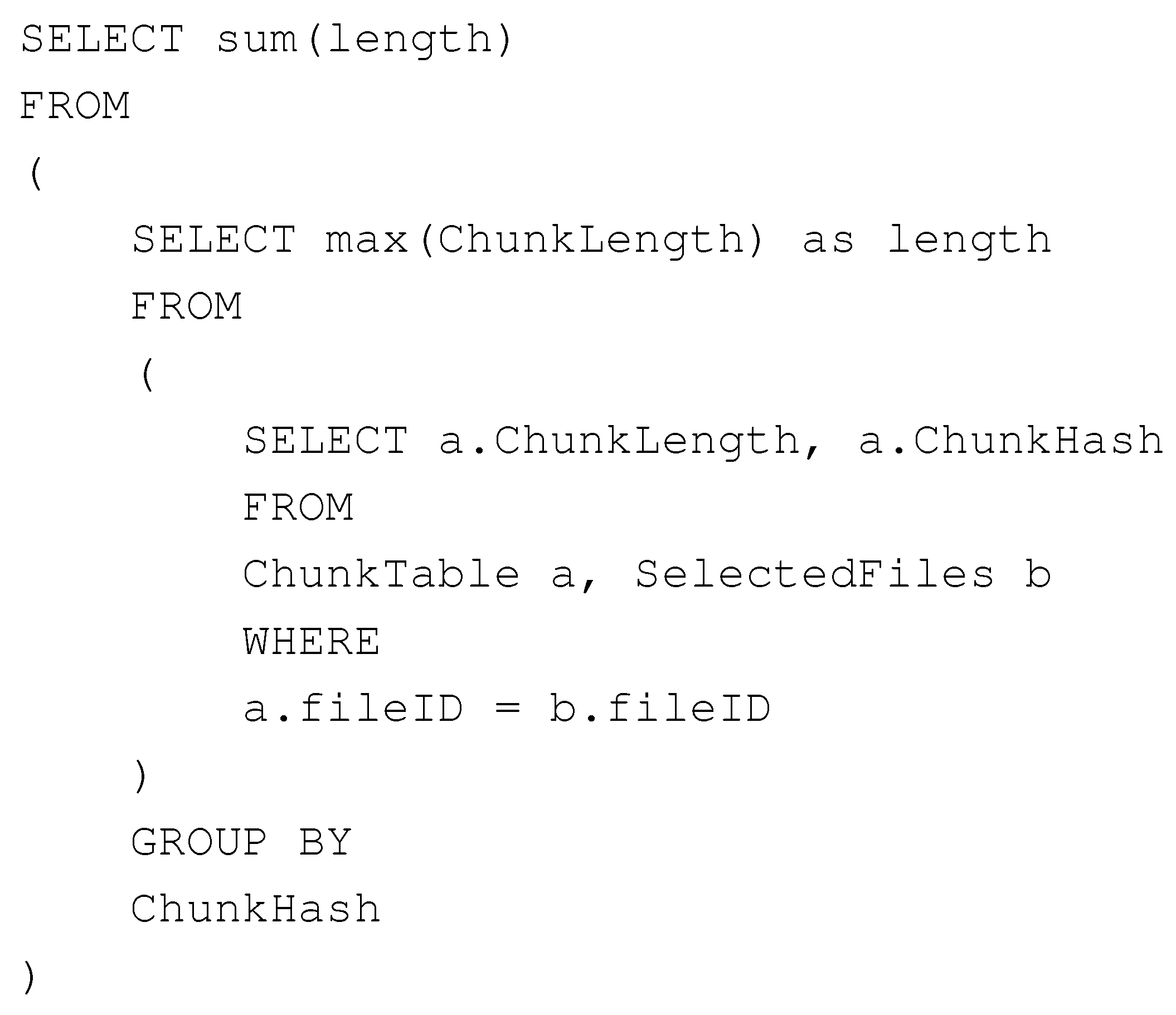
The naive algorithm, denoted as Naive, takes 4 steps to answer on-demand sizequeries. In the first step, Naive initializes the list of files that meet the filtering criteria as a file table called . In the second step, it does an SQL JOIN operation on and to select all tuples for files in , which results in a table
. In the third step, unique chunks in are found by an SQL GROUP BY operation. In the final step, the total size of unique chunks are computed by an SQL SUM operation. All queries in these 4 steps are optimized properly. For example, in step 2, the table has a cluster index on the field so that the SQL JOIN operation is efficient. The SQL query for these 4 steps are shown in Figure 12.
If we assume the number of tuples is N, the number of selected files is S, the number of chunks in these selected files is C, and the number of unique chunks is U, then the complexity of the Naive algorithm in asymptotic notation is given that all involved SQL queries are optimized properly. In particular, step 1 has the complexity of , step 2 has the complexity of , step 3 has the complexity of , and step 4 has the complexity of . Because the Naive algorithm has to scan all chunk tuples in step 2, it is not scalable to the number of chunks. One has to use alternative methods to avoid scanning all chunk tuples. The proposed graph-based algorithm is such an alternative method, and we will describe the details of the algorithm below.
The Graph Algorithm
As described in Section 2.2, a DCSGgraph is created from the deduplication metadata. We use adjacency list to represent edges in the DCSGgraph. Each file vertex is assigned a file identifier , and each unique chunk vertex is assigned a chunk identifier . Note that after deduplication, multiple duplicate chunks map to the same chunk identifier, and we can use the unique chunk identifer to replace the chunk hash value in the algorithm. The DCSGgraph consists of 2 parts: the first part is an indexed and ordered list of pairs, and the second part is a per-vertex adjacency list consisting of pairs, where and represents file size and chunk size, respectively. We modify the original DCSGgraph in two aspects: first, we remove the vertex list of s; second, we add as one attribute of each edge. On one hand, by removing the list, we do not need to query the per- size from the potentially large list, which can become the performance bottleneck for large number of s. On the other hand, by adding chunk size to each edge, the size of the adjacency lists can double from their original form with only s. Given that we can sequentially load the per-file adjacency list into RAM and the average size of per-file adjacency list is considerably small (i.e., <1 MB), the IO overhead in terms of elapsed time is reasonable (<10 ms for hard drives).
Based on the graph representation, the Graph algorithm proceeds with two steps. In the first step, all S selected s and their adjacency lists are fetched from the list to form a DCSGgraph, denoted as B-Graph. The total size of all s are computed, denoted as . The vertex list is implemented as a list, while the vertex list is implemented as a hash table to speed up the lookup performance. In the second step, a breadth-first search (BFS) finds out all s whose degrees are larger than 1, where per- degrees are also recorded. We denote the set of these s as . Each in has their redundant duplicate size as , and the sum of all redundant duplicate sizes are recorded as . The accurate deduplicated size of S files is .
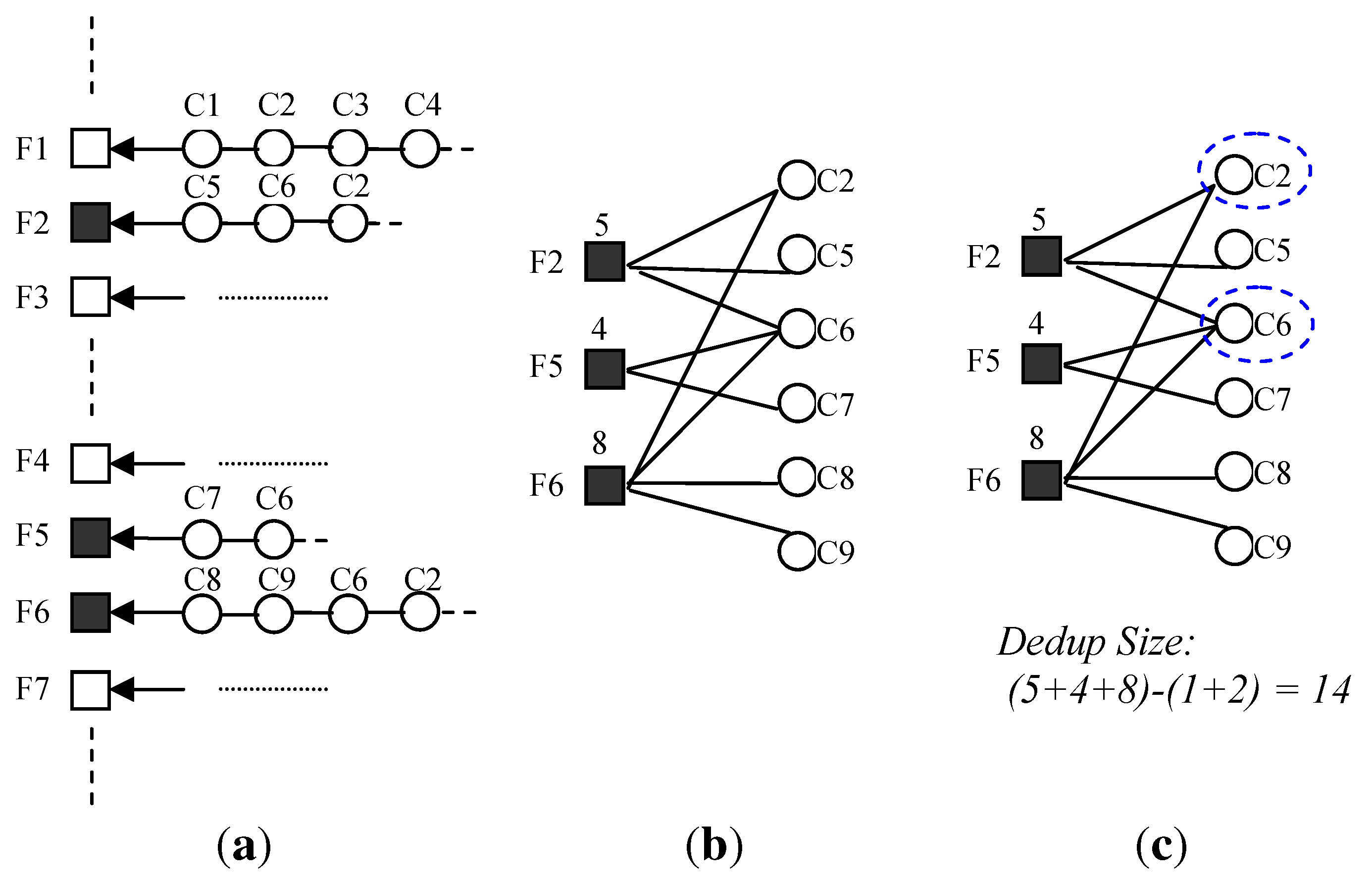
Figure 13 show an example of the Graph algorithm. Initially, each file has a mapping to all its chunks. Each file has its own file size. Each chunk size is 1 so that the edge weight is 1. Chunk identifiers are the result of deduplication so that 2 files can map to the same chunk identifier. For example, appears in file , and . If , and are chosen as the subset of files, in Step 1, these 3 files and its chunks form a B-Graph, , and have their file sizes as 5, 4 and 8, respectively. In Step 2, all chunks are traversed to find out those chunks with more than 1 edge, and are chosen. The accurate deduplicated size of the subset is .
The asymptotic complexity of the Graph algorithm is since step 1 needs to choose S files and step 2 needs to scan C chunks.
The Optimized Graph Algorithm
The Graph algorithm is not scalable with the number of files (and the number of chunks for these files), we propose three optimizations to mitigate the scalability concern. We denote the algorithm with these three optimizations as GraphOpt. The first optimization (OPT-1) is to reduce the number of files and chunks represented in the graph. Note that not all chunks are shared among files, and some files do not share any chunks with other files. These chunks and files do not lead to the inaccuracy of the size computation. We can safely remove them from the graph representation. As shown in Table 5, for WL1, this optimization can reduce the number of s to 56% ( of the original, and the number of s to 8.4% () of the original. For WL2, with this optimization, the number of s drops to 27% () of the original, and the number of s drops to 2% () of the original.
The second optimization (OPT-2) is to aggregate adjacent shared chunks into 1 shared segment to further reduce the number of vertices. The idea behind this optimization is that sharing chunks between two files consists of sequences typically larger than 1 chunk in deduplicated storage systems [12,13]. We define a segment as a range of inter-file shared chunks that appear adjacently and in the same order in all files sharing them. GraphOpt has 2 steps to identify segments. In the first step, each file deduplicates with itself to remove intra-file duplicates, where only the first occurrences of intra-file duplicate chunks are kept. In the second step, GraphOpt employs a straightforward linear algorithm to identify segments. Although more advanced algorithms can be used, such as those based on suffix array [12,14], we developed a straightforward algorithm since the identification of segments occurs only once from the original deduplication metadata. The basic idea behind the straightforward linear algorithm is that segments are identified by two factors, repetition and adjacency. The repetition counter increases when there is a hash value match from inter-file duplicate. The adjacency means that a sequence of chunks with the same repetition are adjacent in all files sharing them. Therefore, any neighboring chunks that do not have the same repetition or are not adjacent in files are not in the same segment, and one can mark the boundary of segments accordingly. For this reason, there are two scans. In the first scan, the boundaries of segments are marked in the array of unique chunks by scanning all chunks from all files. We need an auxiliary data structure to remember the unique chunks and to query the scanned chunks, and we choose a hash table as the auxiliary data structure. With the help of the hash table, we can have an array of unique chunks, upon which we can mark the boundaries of segments. In the second scan, segments are identified by following the marks determined in the first scan.
As shown in Table 5, after applying the first two optimizations, the number of edges drops to 6%–7% of the original number of edges ( for WL1 and for WL2), the number of sub-file vertices drops to less than 1% of the original ( for WL1 and for WL2). The reduction of both edges and sub-file vertices greatly improves the scalability of the DCSGgraph. For example, for a 1 PB deduplicated storage system, if the characteristics of files (e.g., file sizes, chunk sizes) and their sharing are similar, there will be edges and sub-file vertices, which are reasonable numbers to work with.
The third optimization is to make the calculation more stream-friendly. Instead of loading the whole graph into RAM, one can scan shared chunks from selected files one by one. For each new file, the file size after intra-file deduplication is added to . For each chunk that is already in the hash table, , where is the size of the chunk. If the chunk is not in the hash table, it is inserted into the hash table. With this optimization, we do not need to keep the whole graph in RAM. Instead, we only needs to keep the hash table keyed by s in RAM.
Results
In this section, we show the effectiveness of GraphOpt by comparing it with Naive and Graph algorithms. For all three algorithms, the database or graph is assumed to be not cached in RAM initially, and they are stored on external hard drives. At the computation time, the graph or database needs to be loaded into RAM, where RAM is configured to be 1 GB for both graph-based algorithms (i.e., Graph and GraphOpt) and the database-based algorithm (i.e., Naive). For Naive algorithms, we used a commercial database implementation [15] to run the SQL queries. We configured 1 GB for the buffer cache of the database, and we made a fair comparison by tuning the database properly to have a reasonable performance.
For all three algorithms, we varied the percentage of randomly-selected files among all files (denoted as file percentage) and compared their average end-to-end elapsed time of 10 runs to answer on-demand sizequeries. For each file percentage, the same set of files are selected to run on-demand sizequeries for 10 times for each algorithm, and we computed the average elapsed time of these 10 runs for each algorithm. For example, for WL1 and the percentage of 1%, we randomly selected 2893 files out of the total 289,295 files, and use these 2893 files as input to answer on-demand sizequeries for all three algorithms for 10 times.
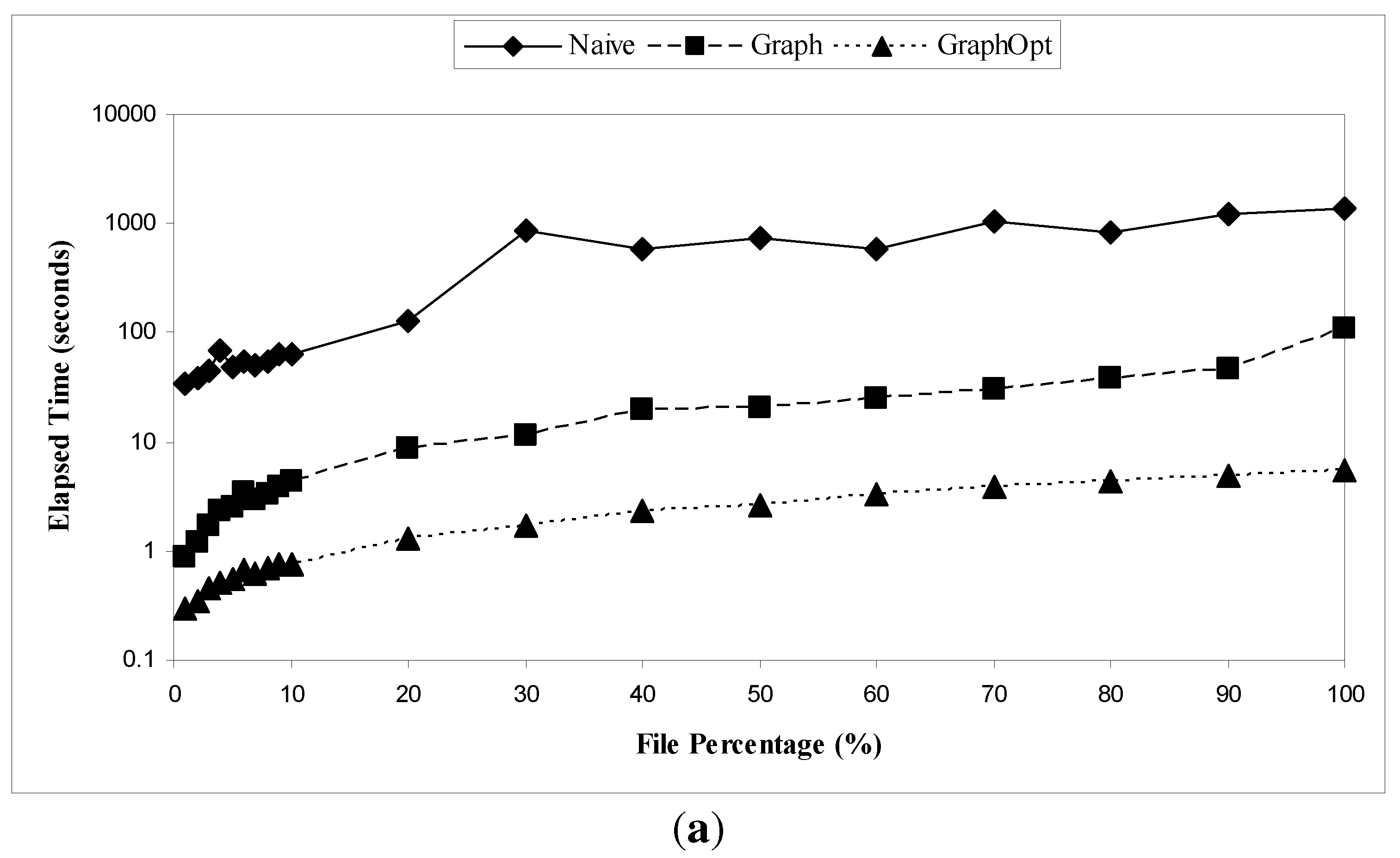
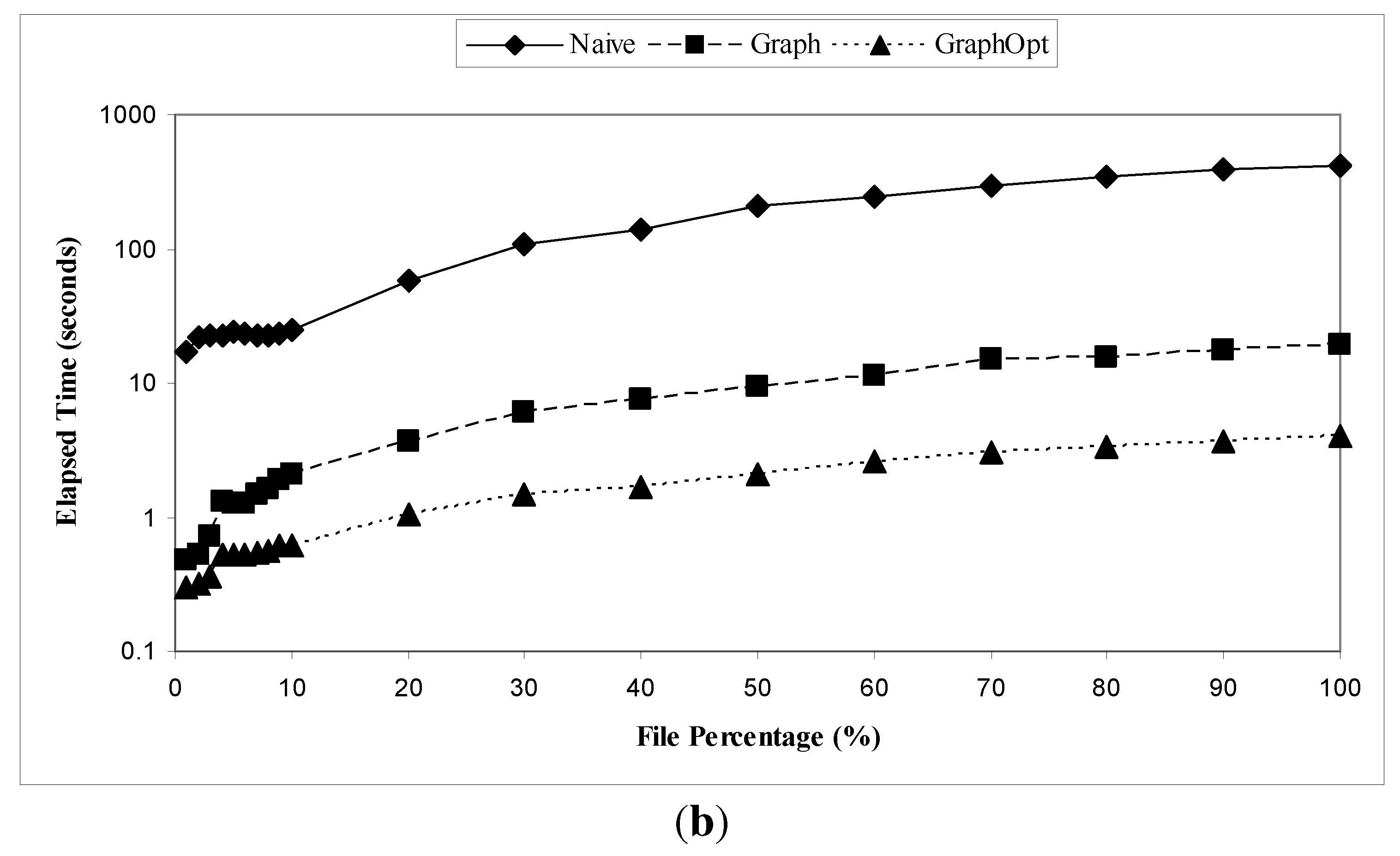
Figure 14(a) and Figure 14(b) show the results of all three algorithms. We can draw two conclusions from the results. First, graph-based algorithms are at least one order of magnitude better than the Naive algorithm with respect to elapsed time. In particular, GraphOpt can achieve the elapsed time less than 1% of what can be achieved from the Naive algorithm. For example, for WL1, when the file percentage is 50%, the elapsed time of Naive is 744 s, the elapsed time of Graph is 21 s, and that of GraphOpt is 2.6 s. Second, GraphOpt is more scalable than Graph. For example, when the file percentage is 10%, both algorithms have an elapsed time less than 5 s. But when the percentage of files is 50%, the Graph algorithm has an elapsed time of 21 s, while the GraphOpt has an elapsed time of 2.6 s.
In Figure 14(a) and Figure 14(b), for both WL1 and WL2, the elapsed time does not increase monotonically with the file percentage for the Naive algorithm because we have no direct control over how the database software scheduled its foreground queries and background activities, which can significantly change the elapsed time. For example, when the file percentage is 30%, the elapsed time is 870 s, but when the file percentage is 40%, the elapsed time is 576 s. But for the other two algorithms, the elapsed time generally increase with the file percentage because larger file percentage reflects larger number of edges, which is a dominant factor of the elapsed time.
4. Discussions of Two Graph Models
Although SCSGand DCSGgraphs both represent the sharing between files, they are different in many aspects. In this section, we describe the two primary differences of these two graph models.
First, compared with DCSG, SCSGgraphs have less vertices and edges, so SCSGgraphs consume less RAM and storage space than DCSGgraphs. For example, for the small sample shown in Table 1, the SCSGgraphs shown in Figure 2 and Figure 3 both have 19 vertices and 19 edges. In comparison, the DCSGgraph shown in Figure 4 has in total 57 vertices (19 File vertices and 38 Chunk vertices), and 184 edges. Even if optimizations such as merging adjacent shared chunks can attenuate the space consumption of DCSGgraphs (see Section 3.3 for details), DCSGgraphs in general consume more RAM or storage space than SCSGgraphs. According to Table 5, with both optimizations, for WL1, the DCSGgraph has 337,602 vertices (162,779 file vertices and 174,823 sub-file vertices) and 1,034,923 edges. Conversely, the SCSGgraph can be 162,779 file vertices and up to 162,778 edges, which are far less than the DCSGgraph. For this reason, SCSGgraphs are more scalable than DCSGgraphs to represent the same set of deduplicated files.
Second, DCSGgraphs are more accurate to some manipulation operations than SCSGgraphs. Such operations included the selection of a sub-graph (including both vertices and edges) from a whole graph, as well as the dynamic modifications of shared content that may end up changing the graph itself. After these manipulation operations, SCSGgraphs may not reflect the accurate sharing, while DCSGgraphs reflect the sharing properly. One example of this inaccuracy is the size computation. For SCSGgraphs, recall the size of a graph is computed by summarizing all vertex weights and then subtracting all edge weights in the graph (due to deduplication), but after partitioning, the size computed in this way is an upper bound of the actual deduplicated size. Take the sample shown in Table 1 for example, if we partition the SCSGgraph with a STAR connection topology in Figure 2 into two sub-graphs G1 and G2, we have and . Based on graphs of G1 and G2, the deduplicated size of G1 is 164 bytes, and the deduplicated size of G2 is 592 bytes. However, in reality, the deduplicated size of G1 is 100 bytes, and the deduplicated size of G2 is 128 bytes. Therefore, after partitioning, the deduplicated size of the sub-graph is not accurate, but an estimate. Note that the estimate is always an upper bound of the actual deduplicated size because in SCSGgraphs, edges are sparse and the sub-graph may miss some edges after manipulation. In this example, for G2, v13 and v14 share 16 bytes, but there is no edge connecting v13 and v14 due to the sparseness of edges. Using the same subgraphs G1 and G2 in the SCSGgraph using the CHAIN connection topology in Figure 3 however, the size estimation is perfect, the deduplicated size of G1 is 100 bytes, and the deduplicated size of G2 is 128 bytes. We could conclude from this made-up experiment that CHAIN connection topology gives much better subgraph size estimate than the STAR connection topology for SCSGgraphs. This is not the case on large scale realistic workloads as we have shown, one reason being that k-cores are not made up of randomly selected vertices. For DCSGgraph as shown in Figure 4, for the same two subgraphs, the deduplicated size of G1/G2 can be computed by adding the sizes of all unique chunks in the sub-graph, so the deduplicated size of G1 or G2 is accurate. Indeed, for DCSGgraphs even for random subgraphs the deduplicated size computation is still accurate (and not an upper bound as for SCSGgraphs).
5. Related Work
We are not aware of any refereed papers using graph representations to optimize or help manage deduplicated storage systems. Also, the concepts of sparse content sharing graphs (SCSG), with their STAR and CHAIN topologies are new. There is a large number of papers related to the deduplication as a data reduction method used in storage systems.
5.1. Storage Deduplication
Deduplication has been maturing as a data reduction technique in both backup storage systems [1,2,4,13,16,17,18] and primary storage systems [19,20]. Kai et al. [18] proposed a method to organize the content hashes in a locality-preserving fashion so as to amortize the cost of loading content hashes when the content hash table cannot fit into the main memory. Lillibridge et al. [13] further reduce the size of the content hash tables by sampling the first hash out of a content hash locality group to fit the content hash table into the main memory. Dong et al. [16] improved the deduplication scope and efficiency by distributing the hash table updates and lookups to multiple nodes. Guo et al. [17] addressed the deduplication scalability issue due to garbage collection by exploiting the incremental nature of the garbage collection in deduplication. Debnath et al. [19] proposed to increase the capacity of the main memory by using the Flash storage. Srinivasan et al. [20] focused on trading-off the deduplication effectiveness with the deduplication latency in primary storage.
These research efforts focus on the optimization of hash updates and lookups because hash updates and lookups are the primary performance and scalability pain points. However, these research efforts in general do not address the problem of the management of deduplicated files. In contrast, our work discusses the challenges and solutions to manage deduplicated files in storage systems.
5.2. Management of Files on Deduplication-Enabled Storage
Management of files have traditionally been the task of the file systems. The management of files is oblivious of their internal sub-file structures, and files are the basic units of file management tasks.
There is a large number of papers in the area of approximate algorithms for graph partitioning, a known NP-complete problem [7]. However, our algorithm based on graph cores is the only linear time approximate algorithm we are aware of. The concept of graph core was introduced by Seidman [8] in studying social networks where it is used to find clusters of densely connected vertices. A linear time algorithm to find cores in a graph is described in Batagelj [21] and our algorithm is an extension considering integer weights for edges rather than just edge degree.
For scalable file subset queries, Leung et al. [10] proposes a scalable metadata search scheme called SpyGlass for large-scale storage systems by exploiting the locality in metadata search queries. Hua et al. [11] took one step further to propose a metadata organization scheme called SmartStore to replace the traditional tree-hierarchy file metadata for large-scale distributed file systems. Similar to SpyGlass, SmartStore adapted the organization of file metadata based on the locality in the metadata search queries. These current research work [10,11] focuses on optimizing the methods to localize the metadata queries, but not about how to get the properties of the resulted subset of files because it is straightforward for non-deduplicated storage. For example, to get the total size of the resulted subset of files, one can simply take the sum of all files in the subset. However, when files are deduplicated, the file management tasks need the help of deduplication metadata because files are related with each other through data sharing. For example, to get the accurate size of a subset of files, one needs to deduplicate the subset of files with the help of the deduplication metadata. A quick method to estimate the deduplicated size of a file system before performing deduplication, thus without knowing the full deduplication metadata, is described by Constantinescu et al. [22].
Unfortunately, there is no standard deduplication metadata format that tracks file sharing among files in deduplication-enabled storage systems. Oracle’s Unified Storage [1], NetApp [2], Windows Server 8 [3] and Celerra of EMC [4] all support deduplication features in storage systems, but these systems keep their deduplication metadata in an ad-hoc fashion internally and do not expose these deduplication metadata externally. Oracle’s Unified Storage [1] and Windows Server 8 [3] keep the deduplication metadata, the mapping from file to sub-file chunks, in the per-file metadata of ZFS and NTFS, respectively. NetApp deduplication for FAS and V-Series [2] stores the deduplication metadata of data volumes in an hidden aggregate volume. Celerra of EMC [4] keeps the deduplication metadata in the per-file metadata. There are other deduplication-enabled storage systems that expose the deduplication metadata. TSM of IBM [23] supports and manages the deduplication in backup storage system. The deduplication metadata in TSM is kept in database tables [5]. Backup Exec of Symantec also stores the deduplication metadata in database tables [6].
To the best of our knowledge, we are not aware of publications that leverage deduplication-based graph models to solve file management tasks in deduplication-enable storage systems. We are the first in the open literature to leverage the deduplication database tables, to adapt them to graphs, and to explore graph-based algorithms to solve real-world file management problems.
6. Conclusions and Future Work
In this paper, we have presented two graph models to represent sharing among files in a deduplicated storage system, and have illustrated and evaluated these two graph models with two real-world applications. One application solved the problem of partitioning a deduplicated set of files into multiple deduplicated subsets with minimal deduplication loss (chunk replication between subsets). The other application measures the actual size of a subset of all files in a deduplicated storage system. Our contributions can be summarized as follows:
- We introduced two novel graph model to represent deduplicated data in a deduplicated storage system. The first graph model represents files as vertices, and sharing between files as edges. This model produces sparse, low memory footprint graphs, a key enabler for efficient graph processing. The second graph model represents files and shared chunks as vertices, and chunk ownership as edges between files and shared chunks. This model produces dense graphs which are resilient to various data manipulation operations in deduplicated storage systems.
- Based on the first graph model, we have designed and evaluated a novel algorithm to partition a deduplication domain based on graph partitioning. This algorithm places the chunks of the same file in the same deduplication domain. For real-world traces, the partition cost (defined as the amount of replicated data over the total amount of removable duplicate data) is less than 6% even when the data is partitioned into 15 domains.
- For the second graph model, we developed optimization methods to mitigate the problem of high memory footprint with various techniques, which proved to be efficient for two real-world traces. In particular, after applying these optimization techniques, the memory footprint can drop to below 10% of the original memory used by DCSGgraphs with no optimization.
- Based on the second graph model, we developed an efficient method to calculate the accurate size of a subset of files from a deduplicated storage system. For the same subset of files, our optimized graph-based algorithm (GraphOpt) has an elapsed time less than 1% of what can be achieved with current methods that access deduplication metadata in a database.
In addition to the partitioning and size-calculation use cases, the graph models and related graph-based algorithms can be applied to other use-cases such as (1) to prevent failure propagation with a minimal deduplication loss and (2) migration of deduplicated files in a tiered-storage environment [24]. We are currently working on these practical problems with the help of expressive graph models and related graph-based algorithms.
Acknowledgment
We would like to thank our summer intern, Abdullah Gharaibeh of UBC, for fruitful discussions, his enthusiasm and help with the data preparation and pre-processing. We are also grateful to our colleague Ramani R. Routray of IBM Research for his insights in IBM’s commercial deduplicated storage systems, and Colin S. Dawson of IBM Software Group, Tucson for his major contributions in collecting the data used in this paper. We want also to acknowledge the enthusiasm and support of our colleagues David Pease and Anurag Sharma for teaching us everything we wanted to know about the revival of tape storage technology.
References
- Oracle Corporation. Bringing Storage Efficiency to a New Level with Oracle’s Unified Storage: Data Deduplication. 2010. Available online: http://www.oracle.com/us/products/servers-storage/sun-storage-7000-efficiency-bwp-065183.pdf (accessed on 30 March 2012).
- NetApp Corporation. NetApp Deduplication for FAS and V-Series Deployment and Implementation Guide: 3.3 Deduplication Storage Savings. 2009. Available online: http://contourds.com/uploads/file/tr-3505.pdf (accessed on 30 March 2012).
- Microsoft Corporation. Data Deduplication in Windows 8 Explained from A to Z. 2010. Available online: http://jeffwouters.nl/index.php/2012/01/disk-deduplication-in-windows-8- explained-from-a-to-z/ (accessed on 30 March 2012).
- EMC Corporation. Achieving Storage Efficiency through EMC Celerra Data Deduplication: Celerra Data Deduplication Overview. 2010. Available online: http://www.emc.com/collateral/hardware/white-papers/h6065-achieve-storage-effficiency-celerra-dedup-wp.pdf (accessed on 30 March 2012).
- IBM Corporation. Implementing IBM Storage Data Deduplication Solutions: 5.7.1 Metadata. 2011. Available online: http://www.redbooks.ibm.com/abstracts/sg247888.html (accessed on 30 March 2012).
- Symantec, Corporation. Backup Exec 2012: Deduplication Option: Deduplication Database Sizing. 2010. Available online: http://www.symantec.com/business/support/resources/sites/BUSINESS/content/live/TECHNICAL_SOLUTION/129000/TECH129694/en_US/351982.pdf (accessed on 30 March 2012).
- Garey, M.R.; Johnson, D.S. Computers and Intractability: A Guide to the Theory of NP-Completeness; W.H. Freeman and Co.: San Francisco, CA, USA, 1979. [Google Scholar]
- Seidman, S.B. Network Structure and Minimum Degree. In Social Networks; Elsevier: New York, USA, 1983; Volume 5, Issue 3, pp. 269–287. [Google Scholar]
- Scott, J.P. Social Network Analysis: A Handbook; Sage Publications: Los Angeles, CA, USA, 2000. [Google Scholar]
- Leung, A.W.; Shao, M.; Bisson, T.; Pasupathy, S.; Miller, E.L. Spyglass: Fast, Scalable Metadata Search for Large-Scale Storage Systems. In Proceedings of the 7th Conference on File and Storage Technologies, San Jose, CA, USA, 24-27 February 2009; USENIX Association: Berkeley, CA, USA, 2009; pp. 153–166. [Google Scholar]
- Hua, Y.; Jiang, H.; Zhu, Y.; Feng, D.; Tian, L. Semantic-aware metadata organization paradigm in next-generation file systems. IEEE Trans. Parallel Distrib. Syst. 2012, 23, 337–344. [Google Scholar] [CrossRef]
- Constantinescu, C. Compression for data archiving and backup revisited. Proc. SPIE 2009, 7444, 1–12. [Google Scholar]
- Lillibridge, M.; Eshghi, K.; Bhagwat, D.; Deolalikar, V.; Trezise, G.; Camble, P. Sparse Indexing: Large Scale, Inline Deduplication Using Sampling and Locality. In Proceedings of the 7th Conference on File and Storage Technologies, San Francisco, CA, USA, 24–27 February 2009; USENIX Association: Berkeley, CA, USA, 2009; pp. 111–123. [Google Scholar]
- Simon, J.; Puglisi, S.J.; Turpin, A.H.; Smyth, W.F. A taxonomy of suffix array construction algorithms. ACM Comput. Surv. 2007, 39, 1–31. [Google Scholar]
- IBM Tivoli. 2011. Available online: http://www.ibm.com/software/tivoli/ (accessed on 30 March 2012).
- Dong, W.; Douglis, F.; Li, K.; Patterson, H.; Reddy, S.; Shilane, P. Tradeoffs in Scalable Data Routing for Deduplication Clusters. In Proceedings of the 9th USENIX Conference on File and Stroage Technologies (FAST ’11), San Jose, CA, USA, 15–17 February 2011; USENIX Association: Berkeley, CA, USA, 2011; p. 2. [Google Scholar]
- Guo, F.; Efstathopoulos, P. Building a High-Performance Deduplication System. In Proceedings of the 2011 USENIX Conference on USENIX Annual Technical Conference (USENIXATC ’11), Portland, OR, USA, 2011, 14–17 June; USENIX Association: Berkeley, CA, USA, 2011; pp. 25–25. [Google Scholar]
- Zhu, B.; Li, K.; Patterson, H. Avoiding the Disk Bottleneck in the Data Domain Deduplication File System. In Proceedings of the 6th USENIX Conference on File and Storage Technologies (FAST ’08), San Jose, CA, USA, 2008, 26–29 February; USENIX Association: Berkeley, CA, USA, 2008; pp. 18–18. [Google Scholar]
- Debnath, B.; Sengupta, S.; Li, J. ChunkStash: Speeding up Inline Storage Deduplication Using Flash Memory. In Proceedings of the 2010 USENIX Conference on USENIX Annual Technical Conference (USENIXATC ’10), Boston, MA, USA, 22–25 June 2010; USENIX Association: Berkeley, CA, USA, 2010; p. 16. [Google Scholar]
- Srinivasan, K.; Bison, T.; Goodson, G.; Voruganti, K. iDedup: Latency-Aware, Inline Data Deduplication for Primary Storage. In Proceedings of the 9th Conference on File and Storage Technologies (FAST ’12), San Jose, CA, USA, 14–17 February 2012. [Google Scholar]
- Batagelj, V.; Zaversnik, M. An O(m) Algorithm for Cores Decomposition of Networks; Technical Report 798; Institute of Mathematics, Physics and Mechanics (IMFM): Ljubliana, Slovenia, 2002. [Google Scholar]
- Constantinescu, C.; Lu, M. Quick Estimation of Data Compression and De-Duplication for Large Storage Systems. In Proceedings of the 1st International Conference on Data Compression, Communication and Processing (CCP ’11), Palinuro, Italy, 21–24 June 2011; pp. 89–93. [Google Scholar]
- IBM Corporation. IBM Tivoli Storage Manager Implementation Guide: Managing Tivoli Storage Manager. 2007. Available online: http://www.redbooks.ibm.com/redbooks/pdfs/sg245416.pdf (accessed on 30 March 2012).
- Guerra, J.; Pucha, H.; Glider, J.; Belluomini, W.; Rangaswami, R. Cost Effective Storage Using Extent Based Dynamic Tiering. In Proceedings of the 9th USENIX Conference on File and Stroage Technologies (FAST ’11), San Jose, CA, USA, 15–17 February 2011. [Google Scholar]
Figure 1.
Content sharing graph for a directory on Windows XP.

Figure 2.
SCSGgraph with STAR connectivity for the small folder with 19 files described in Table 1.
Figure 2.
SCSGgraph with STAR connectivity for the small folder with 19 files described in Table 1.

Figure 3.
SCSGgraph with CHAIN connectivity for the 19 files described in Table 1.
Figure 3.
SCSGgraph with CHAIN connectivity for the 19 files described in Table 1.

Figure 4.
The DCSGgraph for the 19 files described in Table 1.
Figure 4.
The DCSGgraph for the 19 files described in Table 1.

Figure 5.
The k-core decomposition of the SCSGgraph representing the 19 files in Table 1 using CHAIN topology. There are three k-cores: the coreness of ten “red” vertices is 52 bytes, of the five “white” vertices is 20 bytes and of the four “blue” vertices is 16 bytes.
Figure 5.
The k-core decomposition of the SCSGgraph representing the 19 files in Table 1 using CHAIN topology. There are three k-cores: the coreness of ten “red” vertices is 52 bytes, of the five “white” vertices is 20 bytes and of the four “blue” vertices is 16 bytes.

Figure 6.
The k-core decomposition of the SCSGgraph representing the 19 files in Table 1 using STAR topology. There are three k-cores: the coreness of ten “red” vertices is 52 bytes, of the two “white” vertices is 20 bytes and of the seven “blue” vertices is 16 bytes.
Figure 6.
The k-core decomposition of the SCSGgraph representing the 19 files in Table 1 using STAR topology. There are three k-cores: the coreness of ten “red” vertices is 52 bytes, of the two “white” vertices is 20 bytes and of the seven “blue” vertices is 16 bytes.

Figure 7.
The k-cores and their (deduplicated) size for the set of 19 files in Table 1 using CHAIN and STAR topology. There are three k-cores for each connection topology: the top core (value “52”) with (deduplicated) size of 100 bytes, the middle core (value “20”) with size of 124 bytes for CHAIN connectivity and 136 bytes for STAR, and the lower core (value “16”) with size 152 for both connection topologies.

Figure 8.
The k-cores and their (deduplicated) size for WL1 workload using CHAIN and STAR topology.

Figure 9.
Partitioning cost as function of the number of equal sizes partitions, for WL1 workload using CHAIN and STAR topology.
Figure 9.
Partitioning cost as function of the number of equal sizes partitions, for WL1 workload using CHAIN and STAR topology.

Figure 10.
The k-cores and their (deduplicated) size for WL2 workload using CHAIN and STAR topology.
Figure 10.
The k-cores and their (deduplicated) size for WL2 workload using CHAIN and STAR topology.

Figure 11.
Partitioning cost as function of the number of equal sizes partitions, for WL2 workload using CHAIN and STAR topology.
Figure 11.
Partitioning cost as function of the number of equal sizes partitions, for WL2 workload using CHAIN and STAR topology.

Figure 12.
The SQL query of Naive for on-demand sizequeries.

Figure 13.
An example of the Graph algorithm. “Initial State” shows the initial state of the metadata, “Step 1” shows the resulting B-Graph of step 1, “Step 2” shows the computation result. (a) Initial State; (b) Step 1; (c) Step 2.
Figure 13.
An example of the Graph algorithm. “Initial State” shows the initial state of the metadata, “Step 1” shows the resulting B-Graph of step 1, “Step 2” shows the computation result. (a) Initial State; (b) Step 1; (c) Step 2.

Figure 14.
Elapsed times of Naive, Graph, and GraphOpt algorithms for WL1 and WL2, respectively. Y axis is in log scale. (a) WL1; (b) WL2.
Figure 14.
Elapsed times of Naive, Graph, and GraphOpt algorithms for WL1 and WL2, respectively. Y axis is in log scale. (a) WL1; (b) WL2.


Table 1.
Table summarizing the content of the 19 files in the small folder; each file consists of a sequence of four byte blocks (chunks). Chunk 1 is different for each file, but many chunks are common between files. Last column shows the size of each file in bytes, the total size of the 19 files in the directory is 756 bytes.

Table 2.
Workload Summary.
| Workload | WL1 | WL2 |
|---|---|---|
| Total Size | 3,052 GB | 1,532 GB |
| Removable Duplicates | 978 GB | 460 GB |
| Deduplication Ratio | 68% | 70% |
| Number of Files | 289,295 | 201,406 |
| Average File Size | 10 MB | 7.79 MB |
| Median File Size | 82 KB | 18 KB |
| Number of Chunks | 17,509,025 | 12,021,126 |
| Average Chunk Size | 182 KB | 102 KB |
| Median Chunk Size | 71 KB | 52 KB |
Table 3.
The three k-core values and the vertices composing them for each connection topology, CHAIN and STAR, for the 19 files from Table 1. The k-core values represent the minimum bytes shared between any vertices belonging to the core.
Table 3.
The three k-core values and the vertices composing them for each connection topology, CHAIN and STAR, for the 19 files from Table 1. The k-core values represent the minimum bytes shared between any vertices belonging to the core.
| K-Core Value | CHAIN | STAR |
|---|---|---|
| “52” | V1 to V10 | V1 to V11 |
| “20” | “52” and V1 to V15 | “52” and V1, V15 |
| “16” | All Vertics | All Vertics |
Table 4.
Graph Characteristics for workloads WL1 and WL2.
| Workload | WL1 | WL2 |
|---|---|---|
| Number of vertices | 289,295 | 201,406 |
| Number of edges | 327,472 | 246,244 |
| Number of Components | 166,089 | 149,083 |
| Size of Biggest Component | 746. | 1,060. |
Table 5.
Graph characteristics after applying optimization 1 and 2 in GraphOpt for two workloads.
| Workload | WL1 | WL2 |
|---|---|---|
| Num. of File Vertices | 289,295 | 201,406 |
| Num. of Sub-File Vertices | 17,509,025 | 12,021,126 |
| Num. of Edges | 17,509,025 | 12,021,126 |
| Num. of File Vertices with OPT-1 | 162,779 | 55,455 |
| Num. of Sub-File Vertices with OPT-1 | 1,475,780 | 237,235 |
| Num. of Edges with OPT-1 | 8,160,786 | 3,961,316 |
| Num. of File Vertices with OPT-1,2 | 162,779 | 55,455 |
| Num. of Sub-File Vertices with OPT-1,2 | 174,823 | 76,772 |
| Num. of Edges with OPT-1,2 | 1,034,923 | 810,264 |
Publisher’s Note: MDPI stays neutral with regard to jurisdictional claims in published maps and institutional affiliations. |
© 2023 by the authors. Licensee MDPI, Basel, Switzerland. This article is an open access article distributed under the terms and conditions of the Creative Commons Attribution (CC BY) license (https://creativecommons.org/licenses/by/4.0/).
Share and Cite
MDPI and ACS Style
Lu, M.; Constantinescu, C.; Sarkar, P. Content Sharing Graphs for Deduplication-Enabled Storage Systems. Algorithms 2012, 5, 236-260. https://doi.org/10.3390/a5020236
AMA Style
Lu M, Constantinescu C, Sarkar P. Content Sharing Graphs for Deduplication-Enabled Storage Systems. Algorithms. 2012; 5(2):236-260. https://doi.org/10.3390/a5020236
Chicago/Turabian StyleLu, Maohua, Cornel Constantinescu, and Prasenjit Sarkar. 2012. "Content Sharing Graphs for Deduplication-Enabled Storage Systems" Algorithms 5, no. 2: 236-260. https://doi.org/10.3390/a5020236