Stable Flows over Time

Abstract

In this paper, the notion of stability is extended to network flows over time. As a useful device in our proofs, we present an elegant preflow-push variant of the Gale-Shapley algorithm that operates directly on the given network and computes stable flows in pseudo-polynomial time, both in the static flow and the flow over time case. We show periodical properties of stable flows over time on networks with an infinite time horizon. Finally, we discuss the influence of storage at vertices, with different results depending on the priority of the corresponding holdover edges.

1. Introduction

In the stable marriage problem, every vertex of an undirected bipartite graph, G, represents either a woman or a man. Their sympathy for each person of the opposite gender is expressed by their preference lists: the more beloved person has the higher rank. A marriage scheme is a matching, M on G. We say that such a scheme is stable, if there is no pair of participants willing to leave their partners in order to marry each other. More formally: an edge, $uv$, blocks M, if u and v both are unpaired or prefer each other to their partners in M. A matching M is stable, if there is no blocking edge in G. Gale and Shapley [1] were the first to state that a stable matching always exists. Their well-known deferred-acceptance algorithm finds a stable marriage in strongly polynomial time.

One of the most advanced extensions of the stable marriage problem is the stable allocation problem. It was introduced by Baïou and Balinski [2] in 2002. Here, we talk about jobs and machines instead of men and women. Edges have capacity and participants have quota on their matched edges. This quota stands for the time a job needs to get done and the time a machine is able to work in total. Edges are used for assigning jobs to machines, such that none of the machines spends more time on a job than the edge capacity allows them.

The goal is to find a feasible set of contracts, such that no machine-job pair exists where both could improve their states by breaking the scheme. Edge e is blocking, if it is unsaturated, and neither end vertices of e could fill up its quota with at least as good edges as e. An allocation, x, is stable, if none of the edges of G are blocking. Baïou and Balinski [2] give two algorithms to solve the problem: while their augmenting path algorithm runs in strongly polynomial time, the refined Gale-Shapley algorithm is more efficient in simple cases, e.g., on instances where all jobs get one of their best choices, it only needs sublinear time. Dean et al. [3,4] succeeded in speeding up the first method, relying on sophisticated data structures, such as dynamic trees. They also extended the second one to the case of irrational data.

Stable allocations have been further generalized to stable flows by Ostrovsky [5] and Fleiner [6]. Fleiner also gave a constructive proof for the existence of a stable flow in every network by solving a stable allocation problem in a modified network. In an instance of stable flow, special vertices are designated as terminals, and each non-terminal vertex has a preference list of its incoming and outgoing edges that specifies from which edges it prefers to receive flow and which edges it prefers to send flow along. Stable flows are well suited for modeling real-world market situations, as they capture the different trading preferences of vendors and customers.

We extend this model to the setting of flows over time. Flows over time were introduced by Ford and Fulkerson [7,8]. In addition to the stable flow instance, we have transit times on the edges and a time horizon specifying the end of the process. We prove the existence of stable flows over time and, moreover, show that, for the case of an infinite (or sufficiently large) time horizon, there is a stable flow over time, which converges to a static stable flow. By introducing time to the stable flow setting, one can achieve a considerably more realistic and more interesting description of real market situations. With flows over time and transit times on the edges, we can model transportation problems or illustrate distances amongst the vendors.

Structure of the Paper: In Section 2, we introduce the stable flow problem and present an elegant version of the Gale-Shapley algorithm that operates directly on the given network. We also give a simple proof of its correctness. In Section 3, we present the stable flow over time problem and show the existence of stable flows, even in the case of networks with an infinite time horizon. We conclude the section by analyzing how different variations of storage at vertices can influence the stability of flows in a network.

2. Stable Flows

Although most bipartite matching problems can be easily interpreted as network flow problems, stability was defined for flows only in 2008 by Ostrovsky [5]. He proved the existence and some basic properties of stable flows in acyclic networks. Two years later, Fleiner [6] came up with a generalized setting and further results. In this paper, we use this general setting and build upon Fleiner’s remarkable achievements.

2.1. Basic Notions

We consider a network, $(D,c)$, where D is a directed graph, whose vertices $V\left(D\right)$ are partitioned into a set of terminals, $S\subseteq V\left(D\right)$, and non-terminal vertices, $V\left(D\right)\backslash S$. Moreover, there is a capacity function, $c:E\left(D\right)\to {\mathbb{R}}_{>0}$, on the edges. The digraph, D, might contain multiple edges, as well as loops. This concession forces us to slightly modify the structure of the preference lists: each vertex, $v\in V\left(D\right)$, sets up a strictly ordered list of the neighboring edges instead of the neighboring vertices. For convenience, we consider the orderings on incoming and outgoing edges as two separate lists. The set of these lists are denoted by O. Vertex v prefers $uv$ to $wv$, if $uv$ has a lower number on v’s preference list than $vw$. In this case, we say that $uv$ dominates $wv$ at v and denote it by $uv{<}_{v}wv$. The same notation is used for outgoing edges.

Definition 2.1 (flow).

A flow, f, in network, $(D,c)$, is a function, $f:E\left(D\right)\to {\mathbb{R}}_{\ge 0}$, such that the following properties hold:

• $f\left(uv\right)\le c\left(uv\right)$ for all edges, $uv\in E\left(D\right)$;
• ${\displaystyle \sum _{uv\in E\left(D\right)}f\left(uv\right)=\sum _{vw\in E\left(D\right)}f\left(vw\right)}$ for all vertices, $v\in V\left(D\right)\backslash S$.

We would like to emphasize that we do not distinguish sources and sinks in S; their role is the same: they are the vertices in D that do not have to obey the Kirchhoff law.

Definition 2.2 (stable flow).

A blocking walk of flow f is a directed walk, $W=(v_1,e_1,...,e_{k-1},v_k)$, such that all of the following properties hold:

• each edge, $e_i$, $i=1,...,k-1$, is unsaturated;
• $v_1\in S$ or there is an edge, $e^{\prime }=v_{1}u$, such that $f\left(e^{\prime }\right)>0$ and $e_1{<}_{v_1}{e}^{\prime }$;
• $v_k\in S$ or there is an edge, $e^{″}=w{v}_k$, such that $f\left(e^{″}\right)>0$ and $e_{k-1}{<}_{v_k}{e}^{″}$.

A network flow is stable, if there is no blocking walk in the graph.

The network can be seen as a market situation, where the vertices are the traders and the edges connecting them are possible deals. All participants rank their partners for arbitrary reasons: e.g., quality, price or location. These rankings are the preference lists of our instance. Notice that edges do not necessarily correspond to deals involving the same product, and there may be cycles on the graph, even of a length of two. An unsaturated walk is a possible deal between vendors $v_1$ and $v_k$. If they are suppliers or consumers (terminals) or can improve their situation using the unsaturated walk, then they will agree to send some flow along it and break the existing scheme.

It was shown by Fleiner [6] that each instance, $\mathcal{I}$, of the stable flow problem can be converted into an equivalent instance, ${\mathcal{I}}^{\prime }$, of the stable allocation problem, such that every stable flow corresponds to a stable allocation and vice versa. Since there always exists a stable allocation [2], the existence of stable flows directly follows from the equivalence of stability on $\mathcal{I}$ and ${\mathcal{I}}^{\prime }$. The construction shows that stable flows can be found in polynomial time.

Theorem 2.3 

(Fleiner, 2010 [6]). There is a stable flow on every instance, $(D,c,O)$.

Theorem 2.4 

(Fleiner, 2010 [6]). For a fixed instance, each edge incident to a terminal vertex has the same value in every stable flow.

The stable flow problem can be seen as a generalization of the stable allocation problem. We introduce two terminal vertices to G and connect s with all vertices representing jobs and t with all vertices representing a machine. The new edges get the quota of their non-terminal end vertex as capacity. Now, we orient all edges from s to the jobs, from the jobs to the machines and from the machines to t, in order to get a directed network. On this network, all stable flows induce a stable allocation on the original graph and vice versa.

2.2. Algorithms to Find Stable Flows

The stable allocation problem can be solved in polynomial time [2,4]. As mentioned in the introduction, the augmenting path algorithm is not always the most efficient way to find stable allocations; the Gale-Shapley algorithm terminates faster in some cases. It can be run on ${\mathcal{I}}^{\prime }$ in order to give a stable allocation, which yields a stable flow on $\mathcal{I}$. Note that this holds for irrational data, as well. The fact that this method can be directly applied to instance $\mathcal{I}$ is briefly mentioned by Fleiner [6]. In the following, we will show how to interpret the direct application of the Gale-Shapley algorithm on the network as a preflow-push-type algorithm and prove its correctness. We will provide two variants, a basic preflow-push variant that is easy to understand and one that resembles the alternating proposal/refusal scheme of the original Gale-Shapley algorithm.

Proposal and refusal pointers: For each vertex, $v\in V\left(D\right)$, the algorithm maintains two pointers, $p\left[v\right]$ and $r\left[v\right]$. The first pointer, $p\left[v\right]$, iterates through v’s list of outgoing edges from the highest to the lowest priority edge. It points to that edge along which v is currently willing to offer more flow. Likewise, $r\left[v\right]$ iterates through v’s list of incoming edges from the lowest to the highest priority edge. It points to that edge that v is going to refuse next, if necessary. For technical reasons, we introduce one more element to each preference list: after passing through all neighbors, $p\left[v\right]$ reaches a state encoded by $p\left[v\right]=0$. This means that v cannot submit any more offers. Likewise, $r\left[v\right]=0$ initially, as v has no intention to refuse flow in the beginning.

Initialization: The algorithm starts by saturating all edges leaving the terminal set, i.e., $f\left(sv\right)=c\left(sv\right)$ for all $sv\in E\left(D\right)$ with $s\in S$. We define the excess of a vertex, v, w.r.t. f, by $ex(v,f):={\sum }_{uv\in {\delta }^{-}\left(v\right)}f\left(uv\right)-{\sum }_{vw\in {\delta }^{+}\left(v\right)}f\left(vw\right)$, where ${\delta }^{-}\left(v\right)$ denotes the set of incoming edges, while ${\delta }^{+}\left(v\right)$ stands for the outgoing ones. Note that f initially is not a feasible flow, as $ex(v,f)>0$ for some non-terminal vertices, $v\in V\left(D\right)\backslash S$—we will call such vertices active.

Preflow-push variant: The algorithm iteratively selects an active vertex, $v\in V\left(D\right)$, and pushes as much flow as possible along $p\left[v\right]$, advancing the proposal pointer whenever the edge is saturated or an already refused edge is encountered. If $p\left[v\right]$ reaches the zero-state before all excessive flow has been pushed out of the vertex, it continues by decreasing the flow on the incoming edge, $r\left[v\right]$, advancing the refusal pointer whenever the flow on the edge reaches zero. After a push operation, the excess of the vertex is zero, and another active vertex is selected. The algorithm terminates once there is no active vertex left. For a pseudo-code listing of this preflow-push approach, see Algorithm 1.

Algorithm 1 Preflow-push algorithm.

Initialize $p,r$. Saturate all edges, leaving S. while $\exists v\in V\left(D\right)\backslash S:ex(v,f)>0$do     while $ex(v,f)>0$ do         if $p\left[v\right]\ne 0$ then            propose($p\left[v\right]$)         else            refuse($r\left[v\right]$)         end if     end while end while

Simultaneous variant: An alternative variant that resembles the Gale-Shapley algorithm more closely can be obtained by performing alternating rounds of proposal and refusal steps, respectively, on all active vertices simultaneously (cf., Algorithm 2). This variant of the algorithm will prove useful when analyzing stable flows in a time-expanded network later in this paper.

Algorithm 2 Simultaneous push algorithm.

Initialize $p,r$. Saturate all edges, leaving S. while $\exists v\in V\left(D\right)\backslash S:ex(v,f)>0$ do     for all $v\in V\left(D\right):p\left[v\right]\ne 0$ do         propose($p\left[v\right]$)     end for     for all $v\in V\left(D\right):p\left[v\right]=0$ do         refuse($r\left[v\right]$)     end for endwhile

procedurepropose($e=(v,w)$)     if ($r\left[w\right]{>}_{w}e$ or $w\in S$) and $f\left(e\right)<c\left(e\right)$ then         $f\left(e\right):=min\left(f\right(e)+ex(v,f),c(e\left)\right)$     else         advance(p[v])     end if end procedure

procedure refuse($e=(v,w)$)     if $r\left[w\right]\ne 0$ and $f\left(e\right)>0$ then         $f\left(e\right):=max\left(f\right(e)-ex(w,f),0)$     else         advance(r[w])     end if end procedure

A special execution of Algorithm 1 gives the McVitie-Wilson algorithm [9] for the stable marriage problem. We can determine the choice of active vertices, while running Algorithm 1 on the flow instance defined by the stable matching instance. At initialization, the source sends one unit of flow to each vertex, symbolizing a man. The active vertex chosen arbitrarily in the first step is one of them. He proposes along his best edge, and the asked woman accepts the offer and sends the flow further to the sink. Now, the second man will be chosen arbitrarily; he proposes along his best edge. If any woman gets more than one offer, her vertex enters the active set, and she needs to be chosen next. Afterwards, the refused man must play the role of the selected vertex, and so on. This way, we run the deferred-acceptance algorithm by taking the men one by one to the instance, always setting up a current stable matching.

Theorem 2.5. 

If c is integral, both algorithms return an integral stable flow in at most $O\left({\sum }_{e\in E}c\left(e\right)\right)$ iterations.

The proof is split into three parts:

Claim 1. 

Throughout the course of the algorithms, f is integral.

Proof. 

We prove this by induction. The claim is true after initialization, as the capacities of all edges are integral. Thus, before a call of refuse or propose, the excess of the corresponding vertex is integral, as well. This implies that the flow value of the corresponding edge is changed by an integral amount. ☐

Claim 2. 

Both algorithms terminate after $O\left({\sum }_{e\in E}c\left(e\right)\right)$ steps.

Proof. 

In each call of propose, the flow value of the corresponding edge is increased by an integral amount (by claim 1), or the pointer p is advanced. Likewise, in each call of refuse, the flow value of the corresponding edge is decreased by an integral amount, or the pointer r is advanced. Once refuse is called for some edge, $uv$, the flow value cannot be increased by a propose call anymore. Thus, there can be only at most $O\left({\sum }_{e\in E}c\left(e\right)\right)$ calls of propose and refuse. ☐

Claim 3. 

The algorithms return a stable flow.

Proof. 

After termination, f is a feasible flow, as the excess of every non-terminal vertex is zero. Now, suppose there is a blocking walk in the network. There are two reasons for leaving unsaturated edges in the network: either the edge was refused or there was no proposal along it using all its capacity; it stayed at least partly unexamined. We will study which case can come up at which position in the blocking walk.

If an unsaturated walk starts at a terminal vertex, then the first edge of it has been refused, since $s\in S$ must try to fill all its adjacent edges with maximum capacity. If the walk ends at a terminal vertex, there was no full proposal along that edge in the algorithm, since terminal vertices do not refuse any flow. If the blocking walk starts at a non-terminal vertex, then there must be a dominated edge starting at the same vertex and having nonzero value. This proves that the unsaturated edge has been refused, because vertices submit offers along edges in their order in the preference list of the start vertex. A similar argument can applied to the end vertex of the blocking walk: there must be a dominated edge ending at the same vertex and having nonzero value. The unsaturated edge can not be a refused one, since we always refuse the worst edges.

The argument above shows that the blocking walk must start with a refused edge and end with a not fully proposed one. This means that along the walk, there has to be at least one refused edge, $uv$, and an at least partly unexamined one, $vw$. This implies that vertex v refused flow, although it has not filled up its outgoing quota, a contradiction. ☐

Corollary 2.6. 

If c is rational, both algorithms return a rational stable flow.

Proof. 

Any instance with a rational capacity vector can be transformed to an instance with an integral capacity vector by multiplying all capacities with their smallest common denominator. ☐

A simple network setting can illustrate how large capacities may cause a long running time. Note that this example is the flow extension of the allocation problem described by Baïou and Balinski [2].

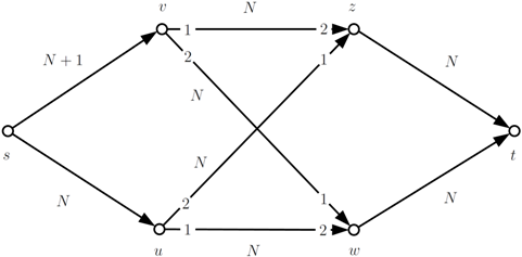
In the example above, $S=\left\{s,t\right\}$, and N is an arbitrary large number. After saturating $sv$ and $su$, the simultaneous push algorithm saturates $uw$ and $vz$ and proposes along $vw$ with one unit. This offer will be accepted by w, forcing it to refuse one flow unit along $uw$. Thus, u has to submit an offer to z, which needs to accept it and reject a flow unit from v. An alternating cycle of new offers and refusals will be made along $v,w,u,z$, as long as there is any flow to refuse along $uw$ and $vz$. This means, in total, N augmentations are along the cycle.

3. Flows over Time

3.1. Basic Notions

We are given a network, $(D,c,\tau )$, consisting of a directed graph, D, some terminal vertices, $S\subseteq V\left(D\right)$, and a capacity function, $c:E\left(D\right)\to {\mathbb{R}}_{>0}$, on the edges. The last element is the transit time function: $\tau :E\left(D\right)\to {\mathbb{Z}}_{\ge 0}$. Besides these, an instance contains a time horizon, $T\in {\mathbb{Z}}_{>0}$, as well. Loops and multiple edges are allowed in D.

Definition 3.1 (flow over time).

Functions, $f_e:\left\{0,1,...,T-1\right\}\to {\mathbb{R}}_{\ge 0}$, for each edge $e\in E\left(D\right)$ form a flow over time or dynamic flow with time horizon, T, if they fulfill all of the following requirements:

• $f_e\left(\theta \right)=0$ for $\theta \ge T-\tau \left(e\right)$
  —this ensures that flow can be sent from u along an edge, $uv$, only if there is enough time left for it to reach v.
• $f_e\left(\theta \right)\le c\left(e\right)$ for all $e\in E\left(D\right)$ and $\theta \in \left\{0,1,...,T-1\right\}$
  —capacity constraints hold all the time.
• ${\displaystyle \sum _{e\in {\delta }^{-}\left(v\right)}{\displaystyle \sum _{\xi \le \theta -\tau \left(e\right)}{f}_e\left(\xi \right)}=\sum _{e\in {\delta }^{+}\left(v\right)}{\displaystyle \sum _{\xi \le \theta }{f}_e\left(\xi \right)}}$ for all $v\in V\left(D\right)\backslash S$ and $\theta \in \left\{0,1,...,T-1\right\}$
  —flow conservation is fulfilled at every point in time.

Any dynamic flow problem can be converted into an ordinary flow problem with the help of the time-expanded network, $D^T$. We create T copies of $V\left(D\right)$, with $v_i$ denoting the $(i+1)$th copy of vertex i. For every edge, $uv\in E\left(D\right)$, and every $i\in \{0,\dots ,T-1-\tau (uv\left)\right\}$, we connect $u_i$ with $v_{i+\tau \left(uv\right)}$. The vertices of $D^T$ with a fixed index, i, form a timeslot. Though this construction reduces the flow over time concept to the static setting without transit times, the price of this simplification is a considerably larger time-expanded network, $D^T$, having a size linear in T and, thus, exponential in the input size. This does not always cause a problem: in the maximum dynamic flow problem, there is always a temporally repeated maximum flow that can be found in polynomial time [7,8].

We extend the flow over a time instance to stable flows over time, by introducing preference lists. They have the same behavior as in the stable flow problem, and they do not change in time. The notion of stability can be extended to this instance the following way:

Definition 3.2 (stable flow over time).

A directed walk, $W=(v^1,e^1,...,e^{k-1},v^k)$, is a blocking walk of flow over time, f, if there is a certain point in time, $0\le \theta \le T-1$, such that all the following properties hold:

• each edge, $e^i$, is unsaturated at time ${\displaystyle \theta +\sum _{j=1}^{i-1}\tau \left(e^j\right)}$
• $v^1\in S$ or there is an edge, $e^{\prime }=v^{1}u$, such that $f_{e^{\prime }}\left(\theta \right)>0$ and $e^1{<}_{v^1}{e}^{\prime }$
• $v^k\in S$ or there is an edge, $e^{″}=w{v}^k$, such that $f_{e^{\prime \prime }}\left({\displaystyle \theta +\sum _{j=1}^{k-1}\tau \left(e^j\right)-\tau \left(e^{\prime \prime }\right)}\right)>0$ and $e^{k-1}{<}_{v^k}{e}^{″}$

A blocking walk, W, can be interpreted in a similar way as in the static case: if the two participants symbolized by the end vertices agree that sending some flow along W would improve their situation, then the scheme will be broken by them.

Note that a flow over time is stable, if and only if the corresponding flow in the time-expanded network is stable in the classical sense.

Theorem 3.3. 

For every $(D,c,\tau ,O)$ and time horizon, $T\in {\mathbb{Z}}_{>0}$, there is a stable flow over time.

Proof. 

A stable static flow exists in the time-expanded network. ☐

Corollary 3.4. 

In every stable flow over time with $T\in {\mathbb{Z}}_{>0}$, the terminal vertices send and receive the same amount of flow in a fixed timeslot on all edges incident to them.

Proof. 

This follows from Theorem 2.4. ☐

Note that these two statements hold, even if the preference lists may change in time.

Remark 3.5. 

Without loss of generality, we can assume the graph to be simple and free of loops. If an edge, e, is a loop or parallel to another edge, we simply split this edge into two edges, $e_1,e_2$, introducing a new vertex, $v_e$. We assign capacities, $c\left(e_1\right)=c\left(e_2\right)=c\left(e\right)$, and transit times, $\tau \left(e_1\right)=\tau \left(e\right)$ and $\tau \left(e_2\right)=0$, to the new edges. As $v_e$ is a non-terminal and has only one incoming and one outgoing edge, it will never be the start or end vertex of a blocking walk. Furthermore, any blocking walk visiting $v_e$ corresponds to a blocking walk in the original graph using the edge, e, and vice versa.

As a result of this assumption, any propose or refuse operation on a vertex, $v_i$, in the time-expanded network does not effect the state of any other copy, $v_j$, of the same vertex.

Time-expanded variant of the preflow-push algorithm: In order to obtain structural insights on stable flows over time, we will apply Algorithm 1 in the time expanded network using a special order of the vertices: it picks a vertex, $v\in V\backslash S$, from the underlying static network and handles all copies of v, starting at $v_0$ and ending at $v_{T-1}$, processing each of them as long as it has excessive flow. We will call such a traversal of all copies of a vertex, v, by the algorithm a v-phase.

The following lemma gives important structural insights on the stable flow computed by Algorithm 3, which will prove useful in the following sections.

Algorithm 3 Time-expanded variant of the preflow-push algorithm.

Initialize $p,r$. Saturate all edges, leaving S. while $\exists v\in V\backslash S:{\sum }_{i=0}^{T-1}ex(v,f)>0$ do     for $i=0$ to $T-1$ do         while $ex(v_i,f)>0$ do            if $p\left[v\right]\ne 0$ then                propose($p\left[v_i\right]$)            else                refuse($r\left[v_i\right]$)            end if         end while     end for end while

Lemma 3.6. 

Let $i<j$. After every u-phase for any vertex, $u\in V\backslash S$, in Algorithm 3, the following statements hold for all $v\in V\left(D\right)\backslash S$:

(a)

$p\left[v_i\right]{\le }_{v}p\left[v_j\right]$

(b)

If $p\left[v_i\right]{=}_{v}p\left[v_j\right]=vw$ and $r\left[w_{j+\tau \left(vw\right)}\right]{>}_{w}vw$ (or $w\in S$), then $f\left(p\left[v_i\right]\right)\le f\left(p\left[v_j\right]\right)$.

(c)

$r\left[v_i\right]{\ge }_{v}r\left[v_j\right]$

(d)

If $r\left[v_i\right]{=}_{v}r\left[v_j\right]\ne 0$, then $f\left(r\left[v_i\right]\right)\ge f\left(r\left[v_j\right]\right)$.

Proof. 

We prove the lemma by induction on the algorithm. Clearly, all statements are true after initialization. We show that they also stay true after the end of each phase.

First, observe that during a u-phase, statements (a) to (d) cannot be invalidated for any vertex, $v\ne u$: The pointers of v are not changed, so (a) and (c) remain valid for v. The flow on any edge, $r\left[v_i\right]$, for any i cannot be changed, so (d) remains valid. Finally $f\left(p\left[v_i\right]\right)$ can only change if $p\left[v_i\right]=r\left[u_{\ell }\right]$ for some index, ℓ, but in this case, (b) is always true. We thus can assume that after a phase of vertex v, statements (a) to (d) are true for all vertices other than v and use this fact to show that they also hold for v.

Let $i<j$, and consider the pointers of copies of vertex u and the flow on their incident edges after a u-phase. As there are no loops in the underlying graph, the algorithm ensures $ex(u_i,f)=ex(u_j,f)=0$. Furthermore:

$$f\left(u_i{w}_{i+\tau \left(e\right)}\right)\ge f\left(u_j{w}_{j+\tau \left(e\right)}\right)\text{for}\text{all}e=uw\in E\text{with}p\left[u_i\right]{>}_{u}uw$$

(1)

(if $u_j{w}_{j+\tau \left(e\right)}$ exists) because (c) and (d) hold for vertex w. Likewise,

$$f\left(w_{i-\tau \left(e\right)}{u}_i\right)\le f\left(w_{j-\tau \left(e\right)}{u}_j\right)\text{for}\text{all}e=wu\in E\text{with}r\left[u_j\right]{>}_{u}wu$$

(2)

(if $w_{i-\tau \left(e\right)}{u}_i$ exists) because (a) and (b) hold for w.

Assume, by contradiction, that (a) or (b) is not valid after the phase. This implies $r\left[u_j\right]=0$ and, thus, $inflow\left(u_i\right)\le inflow\left(u_j\right)$ by Equation (2), where $inflow\left(v\right)={\sum }_{uv\in E\left(D\right)}f\left(uv\right)$. Let $p\left[u_i\right]{=}_{u}e=uw$. If (a) is not valid, then the pointer, $p\left[u_i\right]$, must have been advanced during the phase, and thus, $f\left(p\left[u_i\right]\right)>0=f\left(u_j{w}_{j+\tau \left(e\right)}\right)$. The inequality, $f\left(p\left[u_i\right]\right)>f\left(u_j{w}_{j+\tau \left(e\right)}\right)$, is also true if (b) is not valid. In both cases, $p\left[u_i\right]{\ge }_{u}p\left[u_j\right]$. Thus, by Equation (1), $outflow\left(u_i\right)>outflow\left(u_j\right)$. This yields $ex(u_i,f)<ex(u_j,f)=0$, a contradiction.

Now, assume, by contradiction, that (c) or (d) is not valid after the phase. This implies $p\left[u_i\right]=0$ and, thus, $outflow\left(u_i\right)\ge outflow\left(u_j\right)$ by Equation (1). Let $r\left[u_i\right]{=}_{u}e=wu$. If (c) is not valid, then the pointer, $r\left[u_i\right]$, must have been advanced during the phase, and thus, $f\left(r\left[u_i\right]\right)<f_{\text{old}}\left(w_{i-\tau \left(e\right)}{u}_i\right)\le f_{\text{old}}\left(w_{j-\tau \left(e\right)}{u}_j\right)$, where $f_{\text{old}}$ denotes the flow before execution of the phase. The inequality, $f\left(r\left[u_i\right]\right)<f\left(w_{j-\tau \left(e\right)}{u}_j\right)$, is also true, if (d) is not valid. In both cases, $r\left[u_i\right]{\le }_{u}r\left[u_j\right]$. Thus, by Equation (2), $inflow\left(u_i\right)<inflow\left(u_j\right)$. This again yields $ex(u_i,f)<ex(u_j,f)=0$, a contradiction.

☐

3.2. Infinite Time

In this section, we will prove the existence of a stable flow, even if the time horizon is infinite. This flow can be constructed by applying the time-expanded preflow-push algorithm on $D^{\infty }$ (under the assumption that it can apply the propose and refuse steps on all copies of a vertex in finite time). Even more, after a certain point in time, the stable flow is identical to a temporal repetition of the stable flow computed by the same algorithm in the static network, D.

We define $D_i^{\infty }$ to be the subgraph induced by the vertices, $v_j$ with $j>i$. We will run Algorithm 1 on D and Algorithm 3 on $D^{\infty }$ in parallel, executing a u-phase in $D^{\infty }$ whenever vertex u is processed in D. (Note that the state of vertex $u_i$ does not, in particular, depend on any other vertex copy, $u_j$, with $j>i$. Therefore, the state of $u_i$ and its adjacent edges after the u-phase is well defined, although infinitely many copies of u are processed during the u-phase.) Let f be the flow values in D and $f^{\prime }$ be the flow values in $D^{\infty }$ that occur throughout the run of the algorithm, and let $p,r$ and $p^{\prime },r^{\prime }$ be the corresponding pointers, respectively.

Our main theorem in this section states that there is a point in time from which on all computations in the infinite time expanded network correspond one-to-one to those in the static network.

Theorem 3.7. 

There is a point in time, $0\le i<\infty$, such that at the end of every u-phase for any vertex, u, throughout the course of the algorithm, for every $j\ge i$, $f^{\prime }\left(v_j{w}_{j+\tau \left(vw\right)}\right)=f\left(uv\right)$ for all edges $vw\in E\left(D\right)$, and $p^{\prime }\left[v_j\right]{=}_{v}p\left[v\right]$ and $r^{\prime }\left[v_j\right]{=}_{v}r\left[v\right]$ for all $v\in V\left(D\right)$.

Proof. 

Let ${\tau }_{max}:={max}_{e\in E\left(D\right)}\tau \left(e\right)$. We will first prove by induction that until phase K, the statement of the theorem is true for $i_K:=K·{\tau }_{max}$. Clearly, this is true after initialization, as all edges leaving the terminal set are saturated, and all pointers are at their initial state.

Now assume that after phase K, the state of all flow variables and pointers in $D_{i_K}^{\infty }$ is identical to that in D. Now, let $u\in V\left(D\right)\backslash S$ be the vertex that is processed in the current phase and let $j>i_{K+1}$. Note that before the execution of the u-phase, all edges incident to $u_j$ carry the same flow as all edges incident to u in D (as $j-{\tau }_{max}>i_K$), and $p^{\prime }\left[u_j\right]=p\left[u\right]$ and $r^{\prime }\left[u_j\right]=r\left[u\right]$. Therefore, the u-phase modifies $u_j$ and its incident edges in exactly the same way as u is modified by Algorithm 1 in D. Accordingly, after the end of the u-phase, the statement of the theorem still holds for $i_{K+1}$.

We now have shown that up to phase K, the statement of the theorem holds for $i_K$. Now, let $K_0$ be the number of iterations performed by Algorithm 1 before f is a stable flow in D. After iteration $K_0$, no flow values or pointers in D are changed. Let $i:=i_{K_0+1}$. We will show that after iteration $K_0$, also, no flow values or pointers in $D_i^{\infty }$ are changed, which concludes the proof of the theorem.

After iteration $K_0$, all vertices in $D_i^{\infty }$ are inactive. Thus, their state can only change if the flow value on an edge, $v_k{w}_l$, for $k<i$ and $l\ge i$, is increased. This can only happen, if $f^{\prime }\left(v_k{w}_l\right)<c\left(vw\right)$, as well as $r^{\prime }\left[w_l\right]{>}_{w}vw$, and $p\left[v_k\right]{=}_{v}vw$. Note that at the end of the phase, $K_0$, we have $f^{\prime }\left(v_{k+{\tau }_{max}}{w}_{l+{\tau }_{max}}\right)=f^{\prime }\left(v_k{w}_l\right)$, and $r^{\prime }\left[w_{l+{\tau }_{max}}\right]{=}_w{r}^{\prime }\left[w_l\right]{>}_{w}vw$, by choice of $i=i_{K_0+1}$. Now, by Lemma 3.6, $p\left[v_{k+{\tau }_{max}}\right]{\ge }_{v}p\left[v_k\right]$, and as $v_{k+{\tau }_{max}}{w}_{l+{\tau }_{max}}$ is neither refused nor saturated, $p\left[v_{k+{\tau }_{max}}\right]{=}_{v}vw{=}_{v}p\left[v_k\right]$. Again, by Lemma 3.6, $f^{\prime }\left(v_k{w}_l\right)\le f^{\prime }\left(v_{k+{\tau }_{max}}{w}_{l+{\tau }_{max}}\right)$ as long as neither $p^{\prime }\left[v_{k+{\tau }_{max}}\right]$ nor $r^{\prime }\left[v_{l+{\tau }_{max}}\right]$ are advanced. Therefore, $f^{\prime }\left(v_k{w}_l\right)$ cannot be increased before some vertex in $D_i^{\infty }$ becomes active. Thus, $f^{\prime }\left(v_k{w}_l\right)$ is never increased. ☐

Corollary 3.8. 

Algorithm 3 constructs a stable flow, $f^{\prime }$, in $D^T$, such that $f^{\prime }\left(v_i{w}_{i+\tau \left(vw\right)}\right)=f\left(vw\right)$ for all $vw\in E\left(D\right)$ and all $j\ge (K_0+1)·{\tau }_{max}$, where $K_0$ is the number of iterations performed by the Algorithm 1 to compute the stable flow, f, in D, using the same order of vertices.

3.3. Storing at Vertices

The third point in the definition of a flow over time requires flow conservation in every timeslot. A different model allows storing at vertices: a vendor may delay the shipment of goods at his convenience, as long as the flow arrives at the terminal vertices within the time horizon. More formally, we generalize the definition of the excess of vertex v at time θ as the amount of stored goods at vertex v at time θ:

$${\displaystyle {\text{ex}}_f(v,\theta ):=\sum _{e\in {\delta }^{-}\left(v\right)}{\displaystyle \sum _{\xi \le \theta -\tau \left(e\right)}{f}_e\left(\xi \right)}-\sum _{e\in {\delta }^{+}\left(v\right)}{\displaystyle \sum _{\xi \le \theta }{f}_e\left(\xi \right)}}$$

While strict flow conservation requires ${\text{ex}}_f(v,\theta )=0$ for all non-terminal vertices and times in $\left\{0,...,T-1\right\}$, weak flow conservation allows ${\text{ex}}_f(v,\theta )\ge 0$, except for time $T-1$, where ${\text{ex}}_f(v,T-1)=0$ must hold for all $v\in V\left(D\right)\backslash S$.

The time-expanded network can be adapted for weak flow conservation by introducing so-called holdover edges, $v_i{v}_{i+1}$, of infinite capacity for each $v\in V\left(D\right)$ and $i\in \{0,...,T-2\}$. Setting the ranks of these holdover edges in the preference lists allows the investigation of interesting variations. One intuitive view comes from the fact that storing goods is expensive and people are impatient, thus letting the edges, $v_i{v}_{i+1}$, be the last on $v_i$’s preference list and the first on $v_{i+1}$’s preference list. In the following, we will investigate the four main cases with weak flow conservation, given by varying first and last preferences on the end vertices of holdover edges. In each case, we study how the sets of stable flows obeying the different flow conservation rules are related to each other.

We adapt the definition of a blocking walk for the case of intermediate storing. Apart from a starting time, θ, we need the exact time, ${\theta }_i$, when the walk in D leaves a vertex, $v_i$. A walk in D together with a sequence, $\left\{\theta ,{\theta }_1,{\theta }_2,...,{\theta }_k\right\}$, uniquely determines a walk on $D^T$.

Example 3.9. 

Introducing waiting at vertices, stable flows may lose their stability, independent from the rank of holdover edges.

Proof.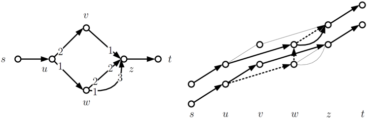 

Consider the following example:

All edges in the static network have unit capacity and unit transit time; s and t are the non-terminal vertices. The unobvious preferences are shown on the edges. The time-expanded network with $T=5$ stands on the right side, showing only the vertices and edges that may be used in a feasible flow. On the static network above, there are three stable flows, each of them uses a different incoming edge of z. If waiting is not allowed, then the dynamic flow shown by the thick edges on the second network is stable, since all unsaturated paths are dominated by it at one end. Adding holdover edges to the time-expanded network breaks the scheme: the walk, $\{u_1,w_2,w_3,z_4\}$ (denoted by dashed lines), blocks the flow over time. Note that this is independent of the rank of the holdover edges, since we only need dominance at the ends of the blocking walk. ☐

Theorem 3.10. 

If T is sufficiently large and holdover edges always stand on the first place on preference lists, then there is no stable flow with value zero on all holdover edges.

Proof. 

Suppose there is a stable flow on the time-expanded network that does not use any of the holdover edges. Consider all the copies of an arbitrary non-terminal vertex, v: if there are two of them that have a positive value on some incoming (and outgoing) edges, then holdover edges between them form a walk that blocks the flow. Thus, a stable flow over time passes through an arbitrary non-terminal vertex, at most, once. Regarding the maximal number of edges with positive flow value, this means two edges, at most, per non-terminal vertex, apart from the terminal-terminal edges that do not affect stability—a flow with this property has positive value on at most $2\left|V\right(D)\backslash S|$ edges in the time-expanded network.

These maximum $2\left|V\right(D)\backslash S|$ edges have to ensure that there is no unsaturated walk between terminal vertices. If the length (w.r.t. transit times) of the shortest walk is denoted by $\tau \left(W_{min}\right)$, then $T-\tau \left(W_{min}\right)+1$ is a lower bound for the number of disjoint walks between terminal vertices. In order to saturate at least one edge along these walks, the inequality, $2|V\left(D\right)\backslash S|\ge T-\tau \left(W_{min}\right)+1$, must hold; otherwise, at least one copy of the shortest walk is unsaturated—hence, it blocks the flow. ☐

Remark 3.11. 

Note that holdover edges can be simulated by introducing loops of unit transit time and sufficiently large capacity at every vertex of the underlying static network. By performing the modification explained in Remark 3.5 on these loops, we obtain an equivalent time-expanded network that fulfills the requirements of Lemma 3.6. We will use this observation in the following theorem.

Theorem 3.12. 

If $T\in {\mathbb{Z}}_{>0}$ and the holdover edges stand on the last place on preference lists, then there is a stable flow that has a value of zero on all holdover edges. It can be computed by applying Algorithm 3 on the time-expanded network, with all holdover edges being split according to Remark 3.11.

Proof. 

By contradiction, assume there is a holdover edge with positive flow value at some vertex, v. W.l.o.g., assume i to be minimal with $f\left(v_i{v}_{i+1}\right)>0$. Since the time horizon is finite, there also is a latest point in time j, such that $f\left(v_j{v}_{j+1}\right)>0$.

Since $f\left(v_i{v}_{i+1}\right)>0$, the pointer, $p\left[v_i\right]$, must already have passed all outgoing non-holdover edges of $v_i$, offering as much flow as the corresponding vertices are willing to accept. Therefore, by Lemma 3.6, the flow on each of these edges must be at least the flow on the corresponding edges of $v_{j+1}$ (if they exist). Thus, the total outflow of $v_i$ exceeds the total outflow of $v_{j+1}$ by at least $f\left(v_i{v}_{i+1}\right)$. On the other hand, $r\left[v_{j+1}\right]$ points either to zero or the incoming holdover edge, and thus, $v_{j+1}$ does not refuse any flow on the regular incoming edges. Again, by Lemma 3.6, the flow on those edges is at least the flow on the corresponding edges of $v_i$. Thus, the total inflow of $v_{j+1}$ exceeds the total inflow of $v_i$ by at least $f\left(v_j{v}_{j+1}\right)$. Putting this together yields $inflow\left(v_{j+1}\right)-outflow\left(v_{j+1}\right)\ge inflow\left(v_i\right)+f\left(v_j{v}_{j+1}\right)-outflow\left(v_i\right)+f\left(v_i{v}_{i+1}\right)>0$, contradicting flow conservation. ☐

In the other two cases, when holdover edges are the best for one of the end vertices and the worst for the other one, storing can be used or avoided, depending on the network. There are even networks where all stable flows have positive value on some holdover edges.

4. Conclusions and Open Questions

We introduced stable flows over time, extending the concept of stability to network flows over time. As initial results, we proved the existence of stable flows, both for finite and infinite time horizons. In both cases, a stable flow can be computed in pseudo-polynomial time by applying a preflow-push algorithm operating directly on the flow network. We also showed that the possibility of storage at non-terminal vertices has an effect on the set of stable flows, depending on the preference given to holdover edges in the time-expanded network.

Although this paper provides first structural insights, many questions brought up by the definition of stable flows over time remain open, most prominently, the complexity of the stable flow problem: Is there a polynomial time algorithm for finding a stable flow? As of today, it is not even clear whether a stable flow over time can be encoded in polynomial space. First, research in this direction indicates that at least the concept of (generalized) temporally repeated flows cannot be applied directly.

Additionally, further extension of stability can be studied on a new setting, e.g., special edges or ties on preference lists, as can be extensions of the flow over the time model, e.g., connections to earliest arrival flows. Finally, we conjecture a stronger form of Theorem 3.12: if holdover edges have lowest priority at both the start and end vertex, no stable flow uses storage at non-terminal vertices.

References

- Gale, D.; Shapley, L. College admissions and the stability of marriage. Am. Math. Mon. 1962, 1, 9–14. [Google Scholar] [CrossRef]
- Baïou, M.; Balinski, M. The stable allocation (or ordinal transportation) problem. Math. Oper. Res. 2002, 27, 485–503. [Google Scholar] [CrossRef]
- Dean, B.C.; Goemans, M.X.; Immorlica, N. Finite termination of “augmenting path" algorithms in the presence of irrational problem data. Algorithms - ESA 2006, 268–279. [Google Scholar]
- Dean, B.C.; Munshi, S. Faster algorithms for stable allocation problems. Algorithmica 2010, 58, 59–81. [Google Scholar] [CrossRef]
- Ostrovsky, M. Stability in supply chain networks. Am. Econ. Rev. 2008, 98, 897–923. [Google Scholar] [CrossRef]
- Fleiner, T. On Stable Matchings and Flows. In Proceedings of the 36th International Workshop on Graph-Theoretic Concepts in Computer Science, Crete, Greece, 28–30 June 2010; Springer-Verlag: Berlin/Heidelberg, Germany, 2010; WG’10, pp. 51–62. [Google Scholar]
- Ford, L.R.; Fulkerson, D.R. Constructing maximal dynamic flows from static flows. Oper. Res. 1958, 6, 419–433. [Google Scholar] [CrossRef]
- Ford, L.R.; Fulkerson, D.R. Flows in Networks; Princeton University Press: Princeton, NJ, USA, 1962. [Google Scholar]
- McVitie, D.G.; Wilson, L.B. The stable marriage problem. Commun. ACM 1971, 14, 486–490. [Google Scholar] [CrossRef]
© 2013 by the authors. Licensee MDPI, Basel, Switzerland. This article is an open access article distributed under the terms and conditions of the Creative Commons Attribution license ( http://creativecommons.org/licenses/by/3.0/).