Appendix
Proof of Lemma 1. If , then for every , we have . Therefore, by F path independence, ; so . Consequently, .
If , then , for every ; so, from substitutability, . Thus, , which means .
By the path independence of F, we have ⇒ ☐
Proof of Lemma 2. We have seen that is monotone; hence .
If , then ; so by the path independency.
Therefore, ; hence . This means S dominates any , i.e., . ☐
The proof of statement 3 is included in the proof of Theorem 11.
Proof of Lemma 5. If is a student of when the score vector is ( i.e., ), then can leave at if she does not reach or got a better opportunity at another college.
If student does not go to college at the score vector, , (), then she will not go to under score vector , because if does not reach , then she does not reach the higher limit, . If reaches , but chooses better college instead, since , she will stay in college . Therefore, the set of students assigned to with is the subset of the set of students going to under . The choice function, , of college is substitutable. Therefore, is valid; then, a subset of it is also valid. Therefore, is -valid. ☐
Proof of Lemma 6. Let the set of contracts above score vectors and be and . Then, . Suppose that for college . Since , from substitutability . Considering the set of contracts of college , , i.e., accepts the same set of contracts with score vector as with . Therefore, . Since G is substitutable, if a set is valid, then its subset is also valid. so . For a smaller set, ; so, is also valid for college .
In other words, if we change the score limit from to , college keeps its score limit, while other colleges may decrease it. Applicants may leave , but no new students will arrive to ; so, score limit is -valid. We can use the same argument for every college; therefore is valid. ☐
In the proofs of Theorems 5 and 6, we use the alternative versions of the score-decreasing/increasing algorithms, where in every step, a college decreases/increases its score limit only by one. These modified algorithms also find stable solutions, as one step of the score decreasing or score increasing can be regarded as several steps of this modified algorithm. From Lemma 5, if score vector is valid and is also valid, then for every , is valid (it is -valid, because is valid, and valid for other colleges, because t is valid). ☐
From the maximal/minimal property of the output solution, we see that the output of the algorithm does not depend on what order by which the colleges modify their score limits. Note that these algorithms may use steps, for example, if we start decreasing from ), but only is a stable score vector.
Proof of Theorem 5. From the algorithm, the fact that no college can decrease its score limit implies that is a stable vector.
Suppose that there exist a stable score vector
, where
. Therefore,
and
, and
for some
i. Define the set:
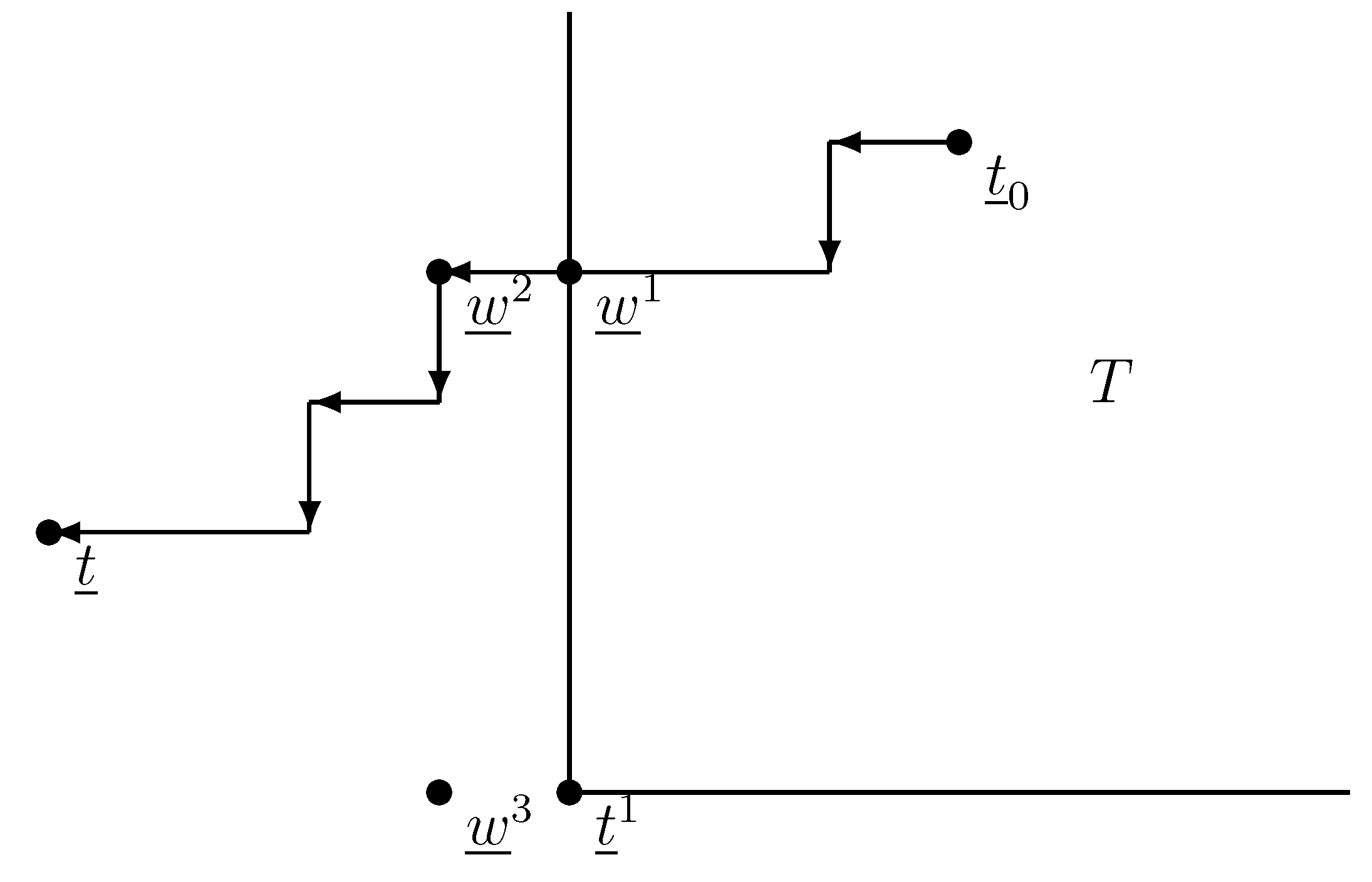
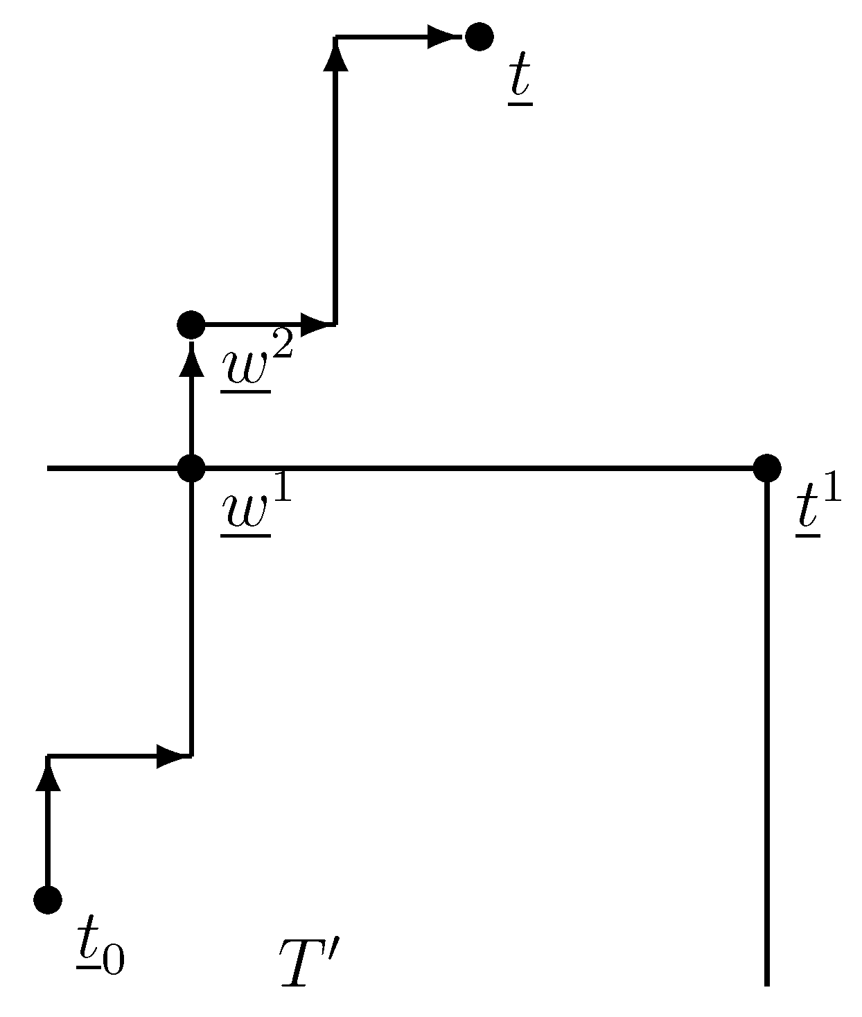
The algorithm starts from and ends in ; so, there is a step, when the score vector leaves T: from score vector , we move to . Since this step is possible, both and are valid score vectors. We know that . Using Lemma 6, both and are valid; so, their minimum is also valid. Therefore, is stable, and it can be reached from by lowering the score limit of . Therefore, is not critical, hence it cannot be stable; a contradiction.
Since every stable score vector are less than or equal to
, the biggest of all stable score vectors is
. Every student is accepted by fewer colleges than in any other stable admissions; so,
is applicant-pessimal.
Figure 6 is showing a possible layout. ☐
Figure 6.
Score-decreasing algorithm.
Figure 6.
Score-decreasing algorithm.
Proof of Theorem 6. It follows from the algorithm that is valid. Suppose that it is not stable, i.e., there is a college, , such that is still valid.
If , look at the step where college raises its score from to , moving from score vector to .
Since the score limits in the algorithm always increase, and ; therefore, . We can use Lemma 5: score limit is valid, so is also -valid. However, then, the algorithm would not have increased to ; a contradiction; Therefore, is stable.
If , since is critical, the score vector is not valid for . From , we get that . Using Lemma 5 again, if was valid, then would be -valid. Therefore, is not valid; therefore, is indeed stable.
To show that
is minimal, suppose that there is a stable score limit,
, such that
, but
,
i.e.,
for some
j. Let:
Since
, but
, there is a step such that when we leave
, we move from
to
. There is a college,
, where
. For other colleges,
; so, by Lemma 5,
was
-stable. Therefore,
does not want to increase its score limit.
Therefore,
is the smallest of all stable score vectors; so, every student gets accepted at as many colleges as possible, and they choose what is best for them. Therefore,
is applicant-optimal.
Figure 7 is showing a possible layout. ☐
Figure 7.
Score-increasing algorithm.
Figure 7.
Score-increasing algorithm.
Proof of Theorem 7. In this proof, we return to the algorithm versions where colleges increase/lower their score limits as much as they can. We call the set of realized contracts at some score vector enrollment.
Each of the n students can go to one of the m colleges or remain unmatched. Therefore, there are at most possible enrollments. In the score-decreasing algorithm, the applicants always change to better. In the score-increasing algorithm, the students’ positions get worse. Therefore, we cannot return to an earlier enrollment in these algorithms.
If we order all enrollments according to the applicants’ preference order, the longest chain contains enrollments. It goes from “everyone gets the best college” to “everyone gets the worst college”. In the score-decreasing algorithm, college may lower its score limit without changing the enrollment, taking the same students as before. If all m colleges do the same, we get the minimal score vector for that given enrollment; next time it came to college , it has to change to a different enrollment or stop. Therefore, in the algorithm, there can be at most m consecutive steps without changing the enrollment. Therefore, the number of steps is .
In the score-increasing algorithm, every step will change the enrollment; hence, if increase its score limit, the set of students going to was infeasible before this step and feasible after the step. Thus, the number of steps is .
Proof of Theorem 11. (i) First, we show that for any given stable set S there is a unique four-stable pair .
Suppose that there are two different stable pairs for S: and .
We can assume that there exists a b for which , but . Since , it follows that . Moreover , but , because .
By , we get ; hence .
We know that and .
Since F is substitutable, contains both sets, ; so, .
From , we get ; so, .
Using that F is path independent, from Theorem 3, . Therefore, ; a contradiction.
Let S and be two different stable sets. Let four-stable pairs and correspond to stable sets S and , respectively.
(ii) ⇒.
From the ordering of the four-stable pairs, and ; so, .
Since F is path independent, from , we get that .
(iii) , ⇒ .
Suppose that . Consequently, , such that , but . From Lemma 2, ; so:
⇒⇒
⇒⇒
We know that ; therefore, . Since F is path independent, ; hence ; a contradiction.
Similarly, from , we get by the monotonicity of and ; hence .
(iv) The stable sets form a lattice.
We have seen that there is an order preserving bijection between the stable sets and stable pairs. As stable pairs form a lattice, stable sets do, as well. ☐
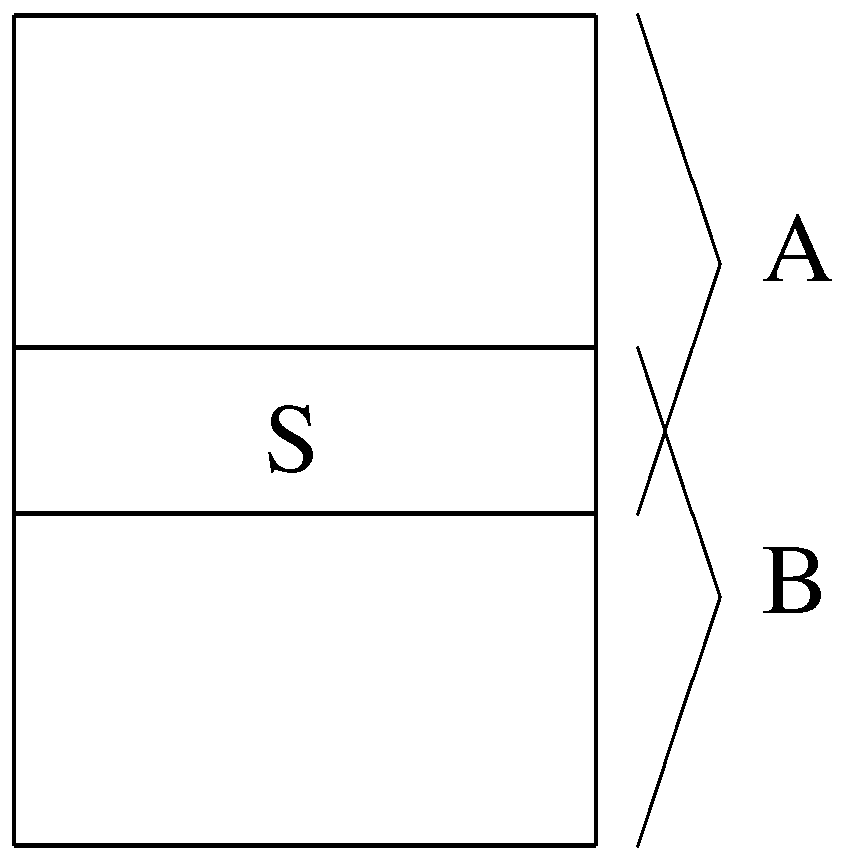
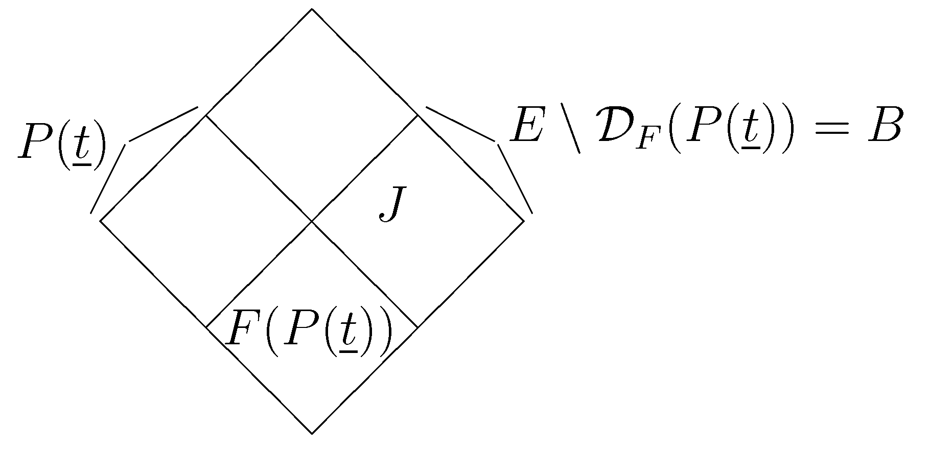
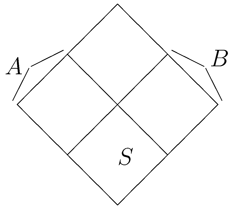
Proof of Statement 5. Let
be the set of contracts that
F prefers to
. In other words,
; therefore,
. (See
Figure 8.)
Suppose is a fixed point. Let , and we use that: . From this,
Since , we get that , and since G is substitutable, . Therefore, ; so, is valid.
To prove that is critical, assume that college lowers its score limit by one. Let
. Then, at college , the accepted increases with some contracts.
Now, we use that the graph is simple. If , then applicant will also be accepted under . If is not accepted at college with score vector , but she has a score of at least , then she will go to if and only if , because she got only one new chance. Therefore, .
Other colleges cannot have new students; so, they stay valid.
From , the scoring function, , for college chooses score limit ; therefore, it also chooses from . Therefore, is not valid.
Now, assume that is valid and critical. Therefore, ; so, accepts contracts in (because contracts in J do not reach score limit ). Therefore, .
As before, . Function P is antitone; so
. Since is monotone, ; so, . As is critical, is infeasible for college ; so, , too, and we get . This is valid for every college; therefore, .
We did not use that is simple in the second direction and in the “valid” part of the first direction; so, these parts remain true for general bipartite graphs. ☐
Figure 8.
Four-partition.
Figure 8.
Four-partition.
Proof of Statement 6. (i)⇒ (ii) If is a fixed point, , then let
As we have seen in the proof of Statement 5, ; so, .
This gives . From the contracts outside B, the set, B, must dominate contracts under score limit , since if colleges do not accept contracts from J, then they will not accept other contracts with the same or lower scores. (It cannot happen that for some college, , all contracts in J have a score of or less and some has a score of , because in that case, would have chosen and would not be stable.) Therefore, . Therefore, .
Since F is path independent and , we get that .
From Lemma 2, ; so, S is indeed four-stable.
(i)⇐ (ii)
If S is four-stable, then there exists , such that . Let the score limit be . We want to know what is. It is sure that , because , and since and , so .
Since , substitutability implies that dominated contracts will not be chosen from , since . Therefore, . Then, . From the path-independent property, .
Using Lemma 2 again, , and ; therefore, is a fixed point. ☐
Proof of Theorem 14. We know from Theorems 5 and 6 that there exist a greatest and a least stable score vector. Let and be two arbitrary stable score vectors. We want to show that they have a join and a meet. Using Lemma 6, is valid. Let us start the score-decreasing algorithm from ; from the algorithm, we get a stable score vector, . From Theorem 5, is the biggest among all the stable score vectors smaller than or equal to . Therefore, , because for every stable vector, such that , ; therefore, .
We finish by showing the existence of . There exists a common upper bound of and , for example . Since the lattice is finite, there has to be at least one least common upper bound. Suppose there exist two least common upper bounds: and . Since is a lower bound of and , ; similarly, . Therefore, we found a common upper bound of and smaller than a; a contradiction. ☐
Proof of Theorem 15. Three-stable ⇒ dominating
There are A and B, such that . From Lemma 1, . The same goes for ; so, . Their union is
.
Additionally, S does not dominate itself; so, .
Dominating ⇒ four-stable
We know that . Let and .
, so . From Lemma 2, . Similarly, . With this pair, S is four-stable.
Four-stable ⇒ three-stable
There exists subsets A and B of E, such that and , and .
Let and .
Now, , , and from Lemma 2, . From Lemma 1, , ; so, with the pair, S is three-stable. ☐
Proof of Theorem 16. In the third part of the proof of Theorem 15, we did not use that G was path independent. ☐
Proof of Theorem 17. Let be the enrollment realized from stable score vector . Define A as the set of contracts above score vector . Let B be the union of S and the set of contracts under score limit .
From all the accepted contracts above score vector , the applicants choose contract set S; so, . If colleges choose from contract set B, just like from all contracts, they would set score limit to ; so, . It is easy to see that ; therefore, S is three-stable. ☐
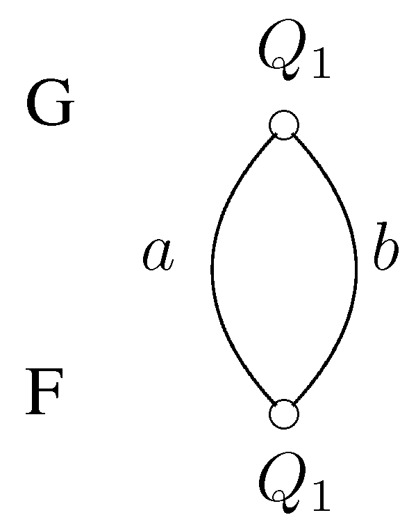
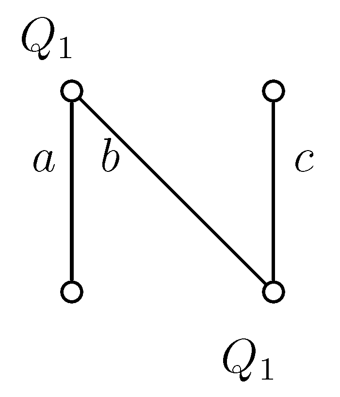
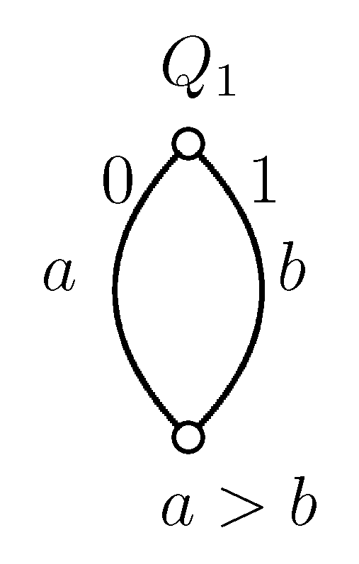
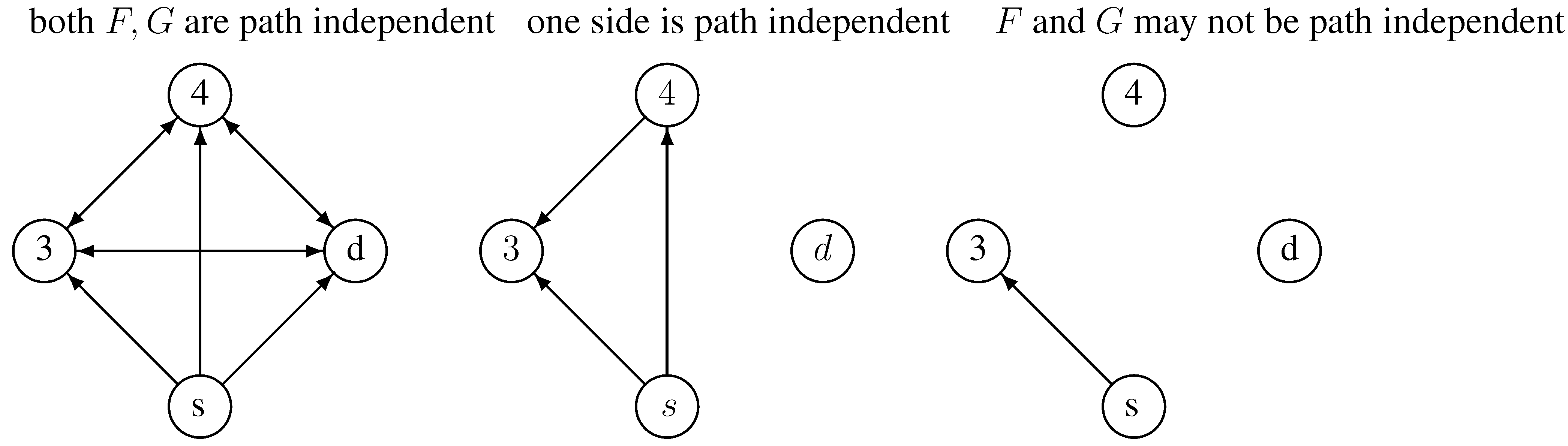
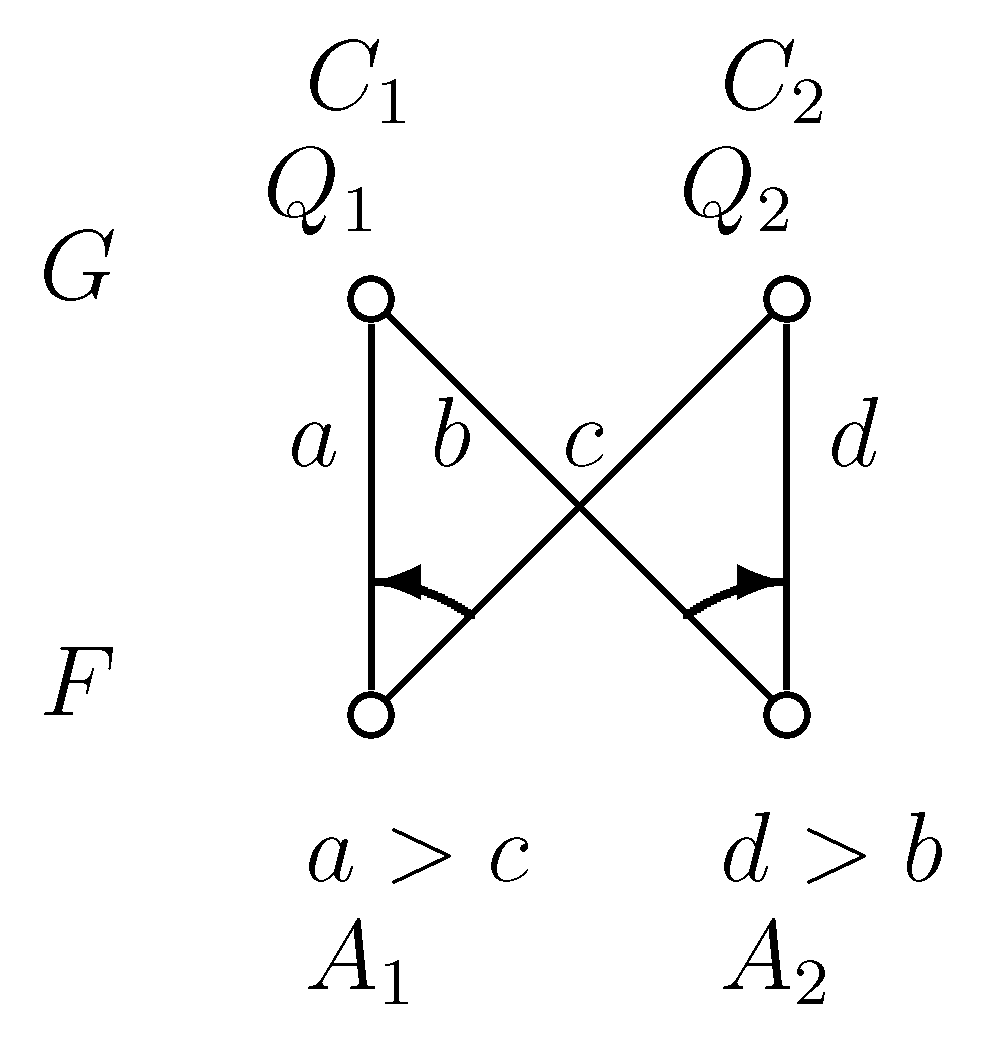
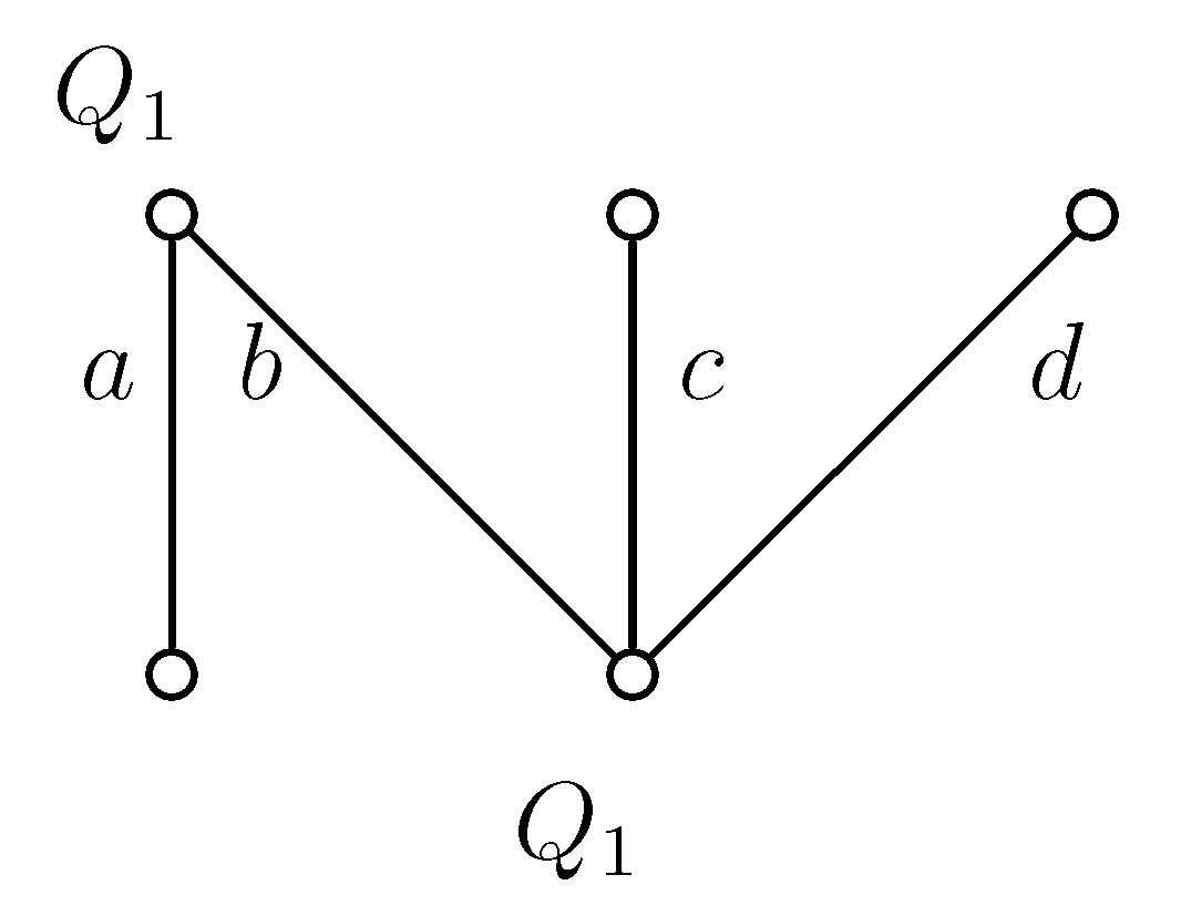
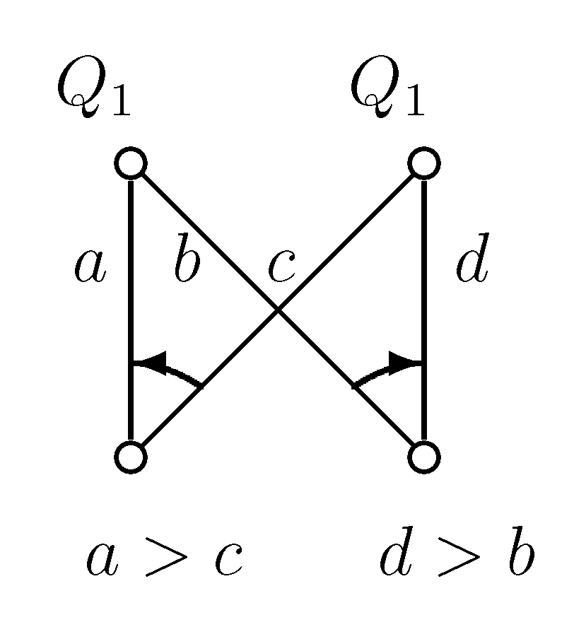
Proof of Statement 7. In
Figure 2 and
Figure 4 and in the following
Figure 9 to
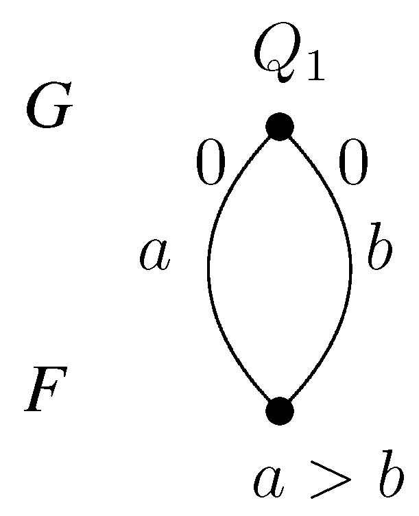
Figure 13, the upper nodes symbolize the colleges, the lower nodes the applicants and the edges between them are the possible contracts. If we write
to a node, that means the given applicant prefers contract
a to
b. In all examples, every student gets a score of zero everywhere, except in
Figure 13, where contract
b has a score of one; so,
b is better for the college.
If a node has only one incident edge, it always chooses that, if it is available.
Figure 9.
Example graph 3.
Figure 9.
Example graph 3.
Figure 10.
Example graph 4.
Figure 10.
Example graph 4.
Figure 11.
Example graph 5.
Figure 11.
Example graph 5.
Figure 12.
Example graph 6.
Figure 12.
Example graph 6.
Figure 13.
Example graph 7.
Figure 13.
Example graph 7.
Table 1 describes the choice functions, usually as a direct sum of the choice functions of individual colleges/applicants. Notation
means a college chooses from equally good contracts
a and
b and its quota is one. We use the abbreviation “path ind." for path independence.
Table 2 shows the stable sets for each notion for the seven examples.
Table 1.
The choice functions for the seven examples.
Table 1.
The choice functions for the seven examples.
| Figure | Simple | | Path ind. | | Path ind. |
|---|
| 2 | no | | no | | no |
| 4 | no | | yes | | no |
| 9 | yes | | yes | | no |
| 10 | yes | | no | | no |
| 11 | yes | | no | | no |
| 12 | yes | | yes | | no |
| 13 | no | | yes | | yes |
Table 2.
Stable sets in case of different stability notions.
Table 2.
Stable sets in case of different stability notions.
| Figure | Three-Stable | Four-Stable | Dominating Stable | Score-Stable | Fixed |
|---|
| 2 | ∅ | | | ∅ | ∅ |
| 4 | | | | | |
| 9 | | | | | |
| 10 | | | | | |
| 11 | | | | | |
| 12 | | | | | |
| 13 | | | | | |


