Article

Algorithm Based on Heuristic Strategy to Infer Lossy Links in Wireless Sensor Networks

1
School of Computer Science and Engineering, Xi'an University of Technology, Xi'an 710048, Shaanxi, China
2
School of Material Science and Engineering, Xi'an Shiyou University, Xi'an 710065, Shaanxi, China
*
Author to whom correspondence should be addressed.
Algorithms 2014, 7(3), 397-404; https://doi.org/10.3390/a7030397
Submission received: 7 May 2014 / Revised: 8 July 2014 / Accepted: 11 July 2014 / Published: 29 July 2014
(This article belongs to the Special Issue Algorithms for Wireless Sensor Networks)

Abstract

:
With the maturing of the actual application of wireless sensor networks, network fault management is eagerly demanded. Severe link packet loss affects the performance of wireless sensor networks, so it must be found and repaired. Subject to the constraints on limited resources, lossy link is inferred using end to end measurement and network tomography. The algorithm based on heuristic strategy is proposed. This maps the problem of lossy links inferences to minimal set-cover problems. The performance of inference algorithms is evaluated by simulation, and the simulation results indicate feasibility and efficiency of the method.

1. Introduction

Lossy link refers to the link which frequently loses packets. With the maturing of wireless sensor network technology, the practical application system of wireless sensor networks gradually appears in many fields, such as environmental monitoring, data collection, etc. Network congestion, too low energy of nodes or wireless communication interferences in wireless sensor networks will result in the loss of severe packets upon linking. Lossy link seriously affects the performance of wireless sensor networks, so it must be found and repaired.
The detecting technology of lossy links is divided into two types: measurement based on collaborative internal nodes and that based on end-to-end nodes. The measurement based on collaborative internal nodes requires each internal node to monitor the packets loss rate of its adjacency link and report it to the sink node. It is straightforward but results in a huge traffic burden, so it is not suitable for wireless sensor networks of limited resources. Each deployed sensor network faces one or some certain applications, in which the node sends application data to the sink node regularly. The technology to infer the performance of links using end-to-end measurement data is called Network Tomography (NT) technology [1]. The advantage of end-to-end measurement is that it does not generate extra monitoring traffic, and this passive measurement does not need extra consumption energy of nodes. Packets loss of application data onto sensor nodes to sink nodes is measured passively using the measurement, and lossy link is inferred using Network Tomography.
Network Tomography currently used to infer lossy links is divided into two types: probing correlations between data packets and scanning single fault. The method of probing correlations between data packets needs to make sure that there are strict correlations between probe packets. Hartl and Li [2] propose that a data collection framework based on data fusion is used to make sure there are correlations between data packets. The method can infer the specific packets loss rate of each link. The method is highly accurate but is difficult to deploy, so the scope of its application is restricted. The method of scanning single faults is mainly used to infer the nature of networks which have a Boolean characteristic, such as network connectivity, lossy link, etc. It assumes there are a few link failures of networks, which lead to packets loss, and do not need correlations between data packets, so it is simple [3]. Padmanabhan et al. [4] propose a Linear Programming (LP) algorithm and Bayesian inference algorithm based on Gibbs sampling. Duffield [5,6] proposes a SCFS inference algorithm based on a greedy strategy. Gibbs’ sampling algorithms have the highest accuracy, but are difficult to apply in inference computation in large-scale network because of high computational cost. SCFS algorithm is simple and its computing speed is very fast, but it tends to give priority to select the links closed to root nodes as lossy links, so it has a big error and can only be used for tree topology. Based on the above research, this paper proposes a heuristic algorithm to infer lossy links, mapping the problem of lossy link inferences to minimal set-cover problems.

2. Network Model

2.1. Topology Model

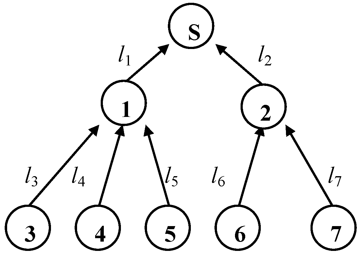
The network logical topology formed into data collection of wireless sensor networks is modeled on reverse trees, T = (V,L), shown in Figure 1. In which, V represents a collection of nodes, L represents a collection of links which connect the nodes. Root nodes of T, named s, represent sink nodes. nv represents the number of nodes, nv = |V|. ne Represents the number of logic links, ne = |L|. Orderly nodes pair (i,j) represents the link between the node i and the node j, (i,j) ∈ V × V, that means the node i is the next hop node of the node j, i is the child node of j in topology T. Link (i,j) ∈ L is shorthanded for li. Any node i has the only father node f(i), except root node s, (i,j) ∈ L, that is j = f(i). Assume that there is a positive integer, n, which establishes the formula k = f n(i), then node k is called the ancestor node of node i, node i is the descendant node of node k. A collection, d(i) = {kV|∃n > 0, i = f n(k)}, represents a descendant nodes collection of the node i. In T = (V,L), the path form the node i to the node s is pi. Set p represents all paths to sink nodes, np = |P| is the number of paths. Mi represents a set of all links which compose path pi.
Figure 1. Schematic diagram of reverse tree network topology.
Algorithms 07 00397 g001
Setting T = (V,L) and P, the routing matrix, A = ( a i j ) n p × n e can be calculated: line i of A corresponds to path pi, row j corresponds to link lj, in which, aij = 1, represents that path pi includes link lj, that is, ljMi. This paper assumes that any link is covered by at least one path.
If the routing between the internal node i and the gather node s in wireless sensor networks has not changed into the data collection periods, topological relations are considered to be stable between the sensor node i and the gather node s. When inferring lossy links, we assume that network topology is known. Network topology can be inferred using end-to-end measurement data if it is not known.

2.2. Performance Model

The performance model used in this paper is described as follows. It puts forward some hypothesis. Suppose that logical topology in sensor networks can keep relatively stable in data collection period TR and that it makes enough data to be collected. Each sensor node in networks sends or forwards sensor data to a sink node. On a sink node it can be perceived that the data of a sensor node reach a sink node. According to sampling frequency of sensor nodes, the number of sending data packets and of loss data packets in transmission path can be known in TR. Suppose that packets loss among the links is independent, following the Bernoulli distribution. The data flow flowing through T, can be described as a random process, Z = (zi,j), id(j), jV. In which, zi,j ∈ {0,1}. zi,j = 1, represents that data sent successfully from the node i arrive the node j, otherwise, data is lost on the link. Suppose ϕk represents average arrival rates of packets of link lk, then the packets loss rate is 1 − ϕk. If path pi consists of m links, that is, Mi = {l1, …, lm}, suppose φi represents average arrival rates of routing packets, then φi= k = 1 m ϕk.
Duffield [7] describes the reason why ϕk has no statistical identification, that is, the packets loss rate of each link can not be calculated using packets loss rate of a path alone, so the link is classified using the threshold value of link packets arrival rate tl as: when ϕk < tl, the link is a lossy link or bad link, otherwise it is not a lossy link. The value of tl can be determined according to specific application requirements or historical data. Ferrari [8] and Kumar [9] show that the link in wireless sensor networks can be clearly distinguished as a good link or bad link. Distinguishability is defined that good paths all consist of good links, and a bad path contains at least one lossy link. Under the assumption that lossy links are relatively rare, the most likely understanding of using end-to-end measurement data to infer the lossy link should be the solution to the minimum number of lossy links.

3. Inference Algorithm

D = {D1, …, Dn} represents a set of end-to-end measurement data. In which, Di = (ri,fi), ri is the number of packets arrived of path pi during measurement, fi is the number of loss packets. Arrival rate of packets of path pi is φi = ri/(ri + fi). Threshold value of packets arrival rates of path pi is set as tp, which can be used to distinguish good or bad path: if φitp, path pi is good, otherwise it is bad. The path set P is divided into good path set pG and bad path set pB according to tp.
tp is set artificially, two kinds of judgment errors are introduced inevitably. False positive error means that good paths are judged on bad paths, and false negative error means that a path is considered to be good but in fact it is bad. When tp = tl is chosen, if a bad link lk (∀lkMi, ϕ l k < tl) exits in path pi, transfer arrival rate of the path is lower than tp (φi = l k M i ϕ l k t l = t p ), at this time there is not exit false positive error. When tp = t l m is chosen (m = |Mi| is the number of links contained in Pi), if the transfer arrival rate of the path is lower than t l m , then there is at least a link whose delivery success rate is less than link tl, so there is no false negative error. When specific distribution of link packets loss rates is not known, the optimal choice of tp cannot be acquired by analysis. This paper chooses tp as (tl + t l m )/2.

3.1. Problem Description

Definition 1: the link control field refers to a path set which contains specified links, that is,
Domain(lk)={pi| piP and lkMi} Domain(lk)={pi| piP and lkMi}
Suppose the most likely solution to lossy links is XL, x is a mark vector whose length is ne, when lkX, xk = 1, otherwise, xk = 0. The problem of lossy link inferences can be described as:
{ m i n m i n z e   l n e x T   s . t .   P R = x = 1 D o m a i n ( l i )
In Formula (1), l n e = {1, 1, … 1} is ne dimensional row vector, so the problems of lossy links inferences can be mapped to minimum set-cover problems. Lossy links can be inferred by solving Formula (1).

3.2. Algorithm Description

The minimal set-cover problem is a typical NP hard problem. SCFS algorithms proposed by Duffield [6] can be seen as a greedy method of solving of set-cover problems. This paper uses the heuristic algorithms to solve it.
Definition 2: path frequency k(i) is the occurrence number of path pi in link control domains sets formed into all links to PB. Suppose piPB, if and only if pi appears in link control domain k, its path frequency is k(i).
Definition 3: link coverage C(i) is the minimum of all paths frequency included in link control domains, Domain(li). That is, C(i) = min{k(j)|PjDomain(li)}.
Definition 4: required links are the links that the coverage is 1.
Definition 5: if the link li is not selected, R required links will appear in alternative links set based on m, required degree of the link li is called R, that is R(i).
Heuristic strategies are proposed using the above definitions, as follows.
Strategy 1: if there is the link li which makes Domain(li) = PB, li is selected as the only lossy link.
Strategy 2: required links must be selected as lossy links.
Strategy 3: if Domain(li) ⊆ Domain(lj), the link li should be excluded.
Strategy 4: if R(i) > R(j), the priority that link li is selected is higher than link lj.
If li is not selected, the number of links which must be selected next is more than the number of links when lj is excluded. The more the required links are, the harder optimization is; it is reasonable to select li. It is a strategy to prevent the algorithm being too greedy.
Strategy 5: the required degree of two links is same, the link selected to control the domain bases should be the higher one. This is a generalization of the simple greedy idea.
Heuristic Lossy Link Inference (HLLI) is described as follows.
Input: Network Topology T(V,L), measurement data set D, threshold value of arrival rate of link packets ti.
(1) Initialization: suppose X is a set of lossy links. X = ϕ, PG = ϕ, PB = ϕ, initialization of mask vectors is zero, that is x = [ 0 , 0 , 0 ] n e .
(2) Calculate tp and arrival rate of link packets for each path in networks, ∀piP, φi = ri/(ri + fi). If φi = tp, PGPG∪{pi}, otherwise, PBPB∪{pi}.
(3) Sets corresponding flag bits to l for constituent links between each path of PB, xi = l, if liMi, piPB.
(4) Calculate path frequency, link coverage and required degree.
(5) While PB ≠ ϕ.
① If the link li exists which make Domain(li) = PB, the link li is added into X, X: = X∪{li}; break;
② If required links exists, the link is added into X: if ∃C(j) = 1 then X: = X∪{lj}, PBPB-Domain(li), continue; otherwise return to ③;
③ ∃li, lj, meet Domain(li) ⊆ Domain(lj), PBPB-Domain{li}, continue; otherwise return to ④;
④ Choose the link that required degree is the highest and add it to X: if ∀xj = 1, ∃li, max R(i), then X: = X∪{lj}, PBPB-Domain(ji), continue; otherwise return to ⑤;
⑤ Select the links that control the biggest domain bases, add it into X.
(6) Output: X.

4. Simulation and Evaluation

Two indicators are used to evaluate the performance of algorithms: Detection Rate (DR) and False Positive Rate (FPD). Set F as a set of actual lossy links in networks, X represents a set of lossy links inferred by algorithms, so the definitions of DR and FPD are:
D R = | F X | | F | ; F P R = | X \ F | | F |
Simulation experiment uses the NS2 network simulation version and uses it to simulate a data gathering algorithm by expanding NS2 in a wireless sensor network. During each round of gathering data, it is determined by random if nodes can successfully get sensor data which is sent from the child nodes. A packets loss rate is set on each link. Emulation and actual packets loss rate tends to presuppose packets loss rate when the round of gathering data gradually increases. The actual number of packets loss on each link is counted to calculate actual packets loss rates of each link with simulation. The accuracy and effectiveness of the algorithm are evaluated by the comparison with the results of inference.
The simulation process constructs tree network using Transit-Stub graphics module generated by GT-ITM Topology Generator. The number of nodes, v, changes in the range of 100~1000. Setting f as the proportion of lossy links in networks, f changes in the range of 0.05~0.25. The definition of packet loss model LM is that the packet loss rate of good links obeys the uniform distribution of the interval [0, 0.01] and the packet loss rate of lossy links obeys uniform distribution of the interval [0.05, 1]. Once a packet loss rate of each link is assigned, the actual process of packets being lost on the link uses the Bernoulli process. The probability of each data packets loss during transmission is determined by the packets loss rate for this link. Each experiment collects data onto 200 rounds, and infers lossy links by measurement data, and calculates DR and FPR of each experiment. The experiment is performed 100 times under each configuration condition, and the advantages and disadvantages of algorithm performance are evaluated by calculating the average value of DR and FPR.
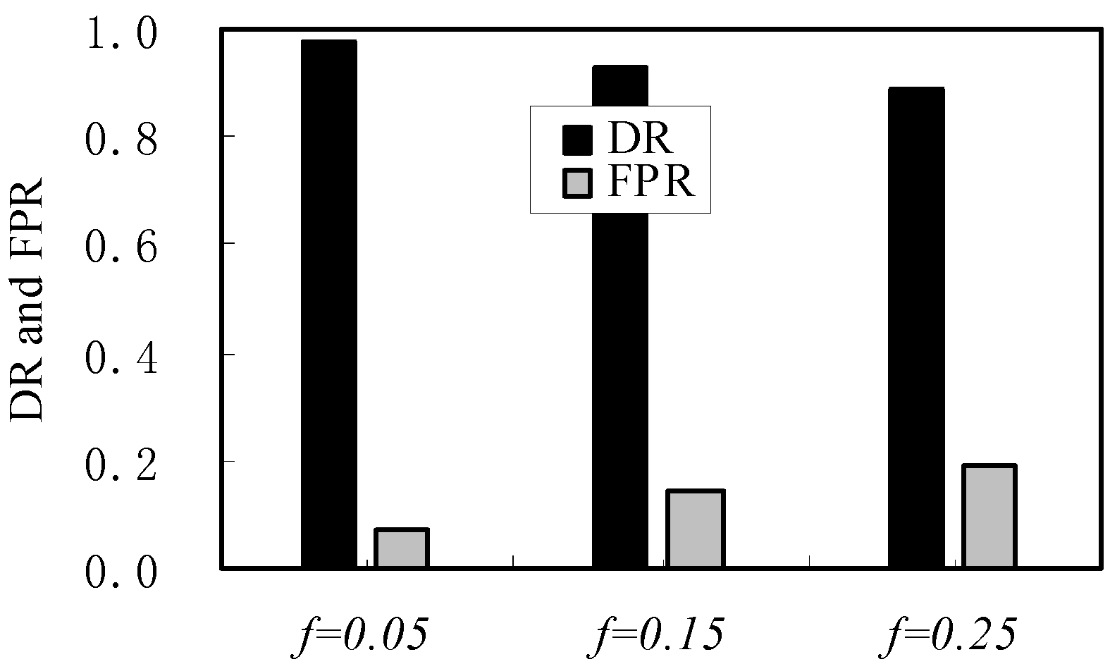
(1) The factor of bad link ratios. The changing trend of algorithm performance is shown as Figure 2 when Network Topology is fixed, the number of nodes v is equal to 500, and the proportion of lossy links, f, changes in the range of [0.05~0.25]. DR decrease, FPR increases, and the algorithm performance reduces as f increases. This trend appears and inference algorithms are built on the assumption that the numbers of lossy links are relatively rare. The assumptions are weakening which leads to a reduction in algorithm performance as the proportion of bad links increases [10,11].
Figure 2. Comparison of performance when f changes, nodes number v = 500.
Algorithms 07 00397 g002
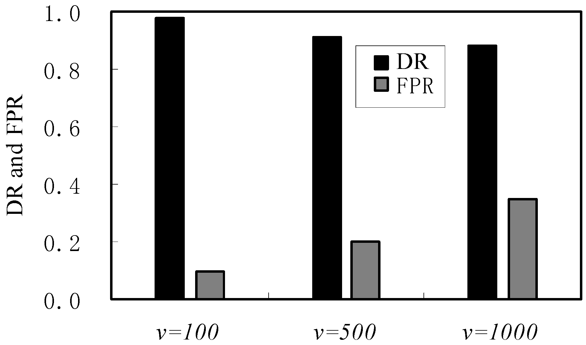
(2) The affect factors of Network Topology. The changing trend of algorithm performance is shown as Figure 3, the proportion of bad links, f, is equal to 0.2, network scales are changed, the number of nodes, v, changes in the range of [100~1000]. As network scales increase, the performance decreases, but the extent of the decrease is much smaller. This means that the algorithm has strong robustness for a change of network scales.
Figure 3. Comparison of performance when the number of nodes changes and f = 0.2.
Algorithms 07 00397 g003
(3) Comparison of SCFS algorithm. The results of comparing HLLI algorithm against SCFS algorithm are shown in Table 1. The coverage of HLLI algorithm is slightly higher than SCFS, but misjudgment rate of HLLI is significantly better than SCFS algorithm. SCFS algorithm uses a greedy strategy based on link control domain bases, and selects the links closed to root nodes as loosy links in the first place. However, the HLLI algorithm can select lossy links more accurately using heuristics strategy.
Table 1. Comparison of performance between Heuristic Lossy Link Inference (HLLI) and Smallest Consistent Failure Set (SCFS).
Performancef = 0.05v = 100f = 0.15v = 500f = 0.25v = 1000
HLLISCFSHLLISCFSHLLISCFS
DR/(%)989893918988
FPR/(%)0.72.01.44.01.96.9

5. Conclusions

Detecting lossy links is an important part of wireless sensor networks management. This method measures application data packets of wireless sensor networks passively, and infers lossy links using the technology of network tomography. This paper proposes a heuristic algorithm of inferring lossy links by mapping the problem of lossy link inferences to minimal set-cover problems, and proves the validity of this algorithm using a simulation experiment.

Acknowledgments

The authors thank the anonymous reviewers for their insightful comments.

Author Contributions

All the authors contributed to the content of this paper. The idea for this research work was proposed by Jing Zhang, the writing of this paper and the design of the algorithm were achieved by Wen-Qing Ma. Both authors discussed the results of the paper before publishing them.

Conflicts of Interest

The authors declare no conflict of interest.

References

  1. Coates, M.; Hero, A.; Nowak, R.; Bin, Y. Internet tomography. IEEE Signal Process. Mag. 2002, 19, 47–65. [Google Scholar] [CrossRef]
  2. Hartl, G.; Li, B. Loss inference in wireless sensor networks based on data aggregation. In Proceedings of the Third IEEE/ACM International Symposium on Information Processing in Sensor Networks (IPSN 2004), Berkeley, CA, USA, 26–27 April 2004.
  3. Khedr, A.M. Minimum connected cover of a query region in heterogeneous wireless sensor networks. Inf. Sci. 2013, 223, 153–163. [Google Scholar] [CrossRef]
  4. Padmanabhan, V.N.; Qiu, L.; Wang, H.J. Server-based inference of internet performance. In Proceedings of the IEEE INFOCOM’03, San Francisco, CA, USA, 1–3 April 2003.
  5. Duffield, N.G. Simple network performance tomography. In Proceedings of the IMC’03, Miami Beach, FL, USA, 27–29 October 2003.
  6. Duffield, N.G. Network tomography of binary network performance characteristics. IEEE Trans. Inf. Theory 2006, 52, 5373–5388. [Google Scholar] [CrossRef]
  7. Duffield, N.; Horowitz, J.; Presti, F.L.; Towsley, D. Multicast topology inference from measured end-to-end loss. IEEE Trans. Inf. Theory 2002, 48, 26–45. [Google Scholar] [CrossRef]
  8. Ferrari, G. Information fusion in wireless sensor networks with source correlation. Inf. Fusion 2014, 15, 80–89. [Google Scholar] [CrossRef]
  9. Kumar, N. An advanced energy efficient data dissemination for heterogeneous wireless sensor networks. Sens. Lett. 2013, 11, 1771–1778. [Google Scholar] [CrossRef]
  10. Srinivasan, K.; Jain, M.; Choi, J.I.; Azim, T.; Kim, E.S.; Levis, P.; Krishnamachari, B. The κ-Factor: Inferring protocol performance using inter-link reception correlation. In Proceedings of the 16th Annual International Conference on Mobile Computing and Networking (Mobicom), Chicago, IL, USA, 20–24 September 2010.
  11. Khreishah, A.; Khalil, I.; Wu, J. Distributed network coding based opportunistic routing for multicast. In Proceedings of the ACM Mobihoc, Hilton Head, SC, USA, 11–14 June 2012.