
A Novel Complex-Valued Encoding Grey Wolf Optimization Algorithm

1
College of Information Science and Engineering, Guangxi University for Nationalities, Nanning 530006, China
2
Key Laboratory of Guangxi High Schools Complex System and Computational Intelligence, Nanning 530006, China
*
Author to whom correspondence should be addressed.
Algorithms 2016, 9(1), 4; https://doi.org/10.3390/a9010004
Submission received: 6 November 2015
/
Revised: 8 December 2015
/
Accepted: 10 December 2015
/
Published: 30 December 2015
Abstract
:Grey wolf optimization (GWO) is one of the recently proposed heuristic algorithms imitating the leadership hierarchy and hunting mechanism of grey wolves in nature. The aim of these algorithms is to perform global optimization. This paper presents a modified GWO algorithm based on complex-valued encoding; namely the complex-valued encoding grey wolf optimization (CGWO). We use CGWO to test 16 unconstrained benchmark functions with seven different scales and infinite impulse response (IIR) model identification. Compared to the real-valued GWO algorithm and other optimization algorithms; the CGWO performs significantly better in terms of accuracy; robustness; and convergence speed.
1. Introduction
Over the last few decades, various heuristic optimizations have been developed to solve complex computational problems. Some of the most popular are: particle swarm optimization (PSO) [1], genetic algorithm (GA) [2], differential evolution (DE) [3,4], simulated annealing (SA) [5], ant colony optimization (ACO) [6], artificial bee colony optimization (ABC) [7], gravitational search algorithm (GSA) [8,9], charged system search (CSS) [10], magnetic optimization algorithm (MOA) [11], biogeography-based optimization algorithm (BBO) [12,13], and teaching learning-based optimization (TLBO) [14]. The swarm intelligence optimization algorithm can flexibly and effectively deal with different problems that conventional optimization techniques cannot solve. For this reason, optimization techniques have been widely used in many domains of study. In addition, it has been demonstrated that there is no heuristic optimization that can solve all optimization problems [15]. In other words, existing algorithms give satisfactory results in solving some problems, but not all problems. Therefore, several new heuristic algorithms are proposed every year, and research in this field is active.
The real-value grey wolf optimization (GWO) is a new population-based meta-heuristic approach initially proposed by Mirjalili et al. (2014) [16]. Due to the fact that the GWO algorithm is simple, flexible and efficient, it can be successfully applied to practical applications [17,18,19]. There are many modified versions of the GWO algorithm. For example, some people study the parameters of the GWO algorithm or combine the GWO algorithm with other heuristic optimization algorithms. However, these methods all use binary or decimal encoders to position the grey wolf, the individual gene contains information to be limited.
The complex-valued encoding method has been applied in expressing neural network weights [20] and representing individual genes for evolutionary algorithms [21]. It uses a diploid to express genes and greatly expand the information capacity of the individual. Starting from the individual encoding method, this article studies the improvement of the performance of the grey wolf with the complex-valued method. The value of the independent variables for an objective function is determined by modules and the signthe independent variables is determined by angles. For the GWO algorithm, the grey wolf individual is divided into two parts, namely: a real part gene and an imaginary gene. Additionally, the two parts represent a variable being able to enhance the information of a grey wolf individual and a diverse population, avoiding the local optimum. Based on the above advantages, we provide a new method for the GWO algorithm to solve practical problems.
The rest of the paper is organized as follows: Section 2 presents a brief introduction to GWO. Section 3 discusses the basic principles of a complex-valued version of GWO. The experimental results of test functions and infinite impulse response (IIR) system identification problem are shown in Section 4 and Section 5, respectively. Finally, Section 6 concludes the work and suggests some directions for future study.
2. Grey Wolf Optimization (GWO)
The GWO algorithm simulates the hunting and social leadership of grey wolves in nature [16]. The algorithm is simple, robust, and has been used in various complex problems. In the GWO algorithm, the colony of grey wolves is divided into four groups: alpha (), beta (), delta (), and omega (). In every iteration, the first three best candidate solutions are named , , and . The rest of the grey wolves are considered as , and are guided by , , and to find the better solutions. The mathematical model of the wolves’ encircling process is as follows [16]:
where indicates the current iteration, , , is the position vector of the prey, indicates the position vector of a grey wolf, is gradually decreased from 2 to 0, and , are random numbers over range .
It should be noted here that, during optimization, the wolves update their positions around , , and . Therefore, wolves are able to reposition with respect to , , and . The mathematical model of wolves readjusting the positions is as follows [16]:
where is the position of the alpha, is the position of the beta, is the position of the delta, , , and , , are all random vectors, is the position of the current solution, and indicates the number of iterations.
As mentioned before, wolves update their positions based on positions of , , and . There are two vectors: and that are random and adaptive vectors which help the algorithm to escape from local optima. When , half of the iterations are devoted to exploration. The range of is . The vector also improves exploration when . In contrast, the other half of the iterations are dedicated to exploitation when , and the exploitation is also emphasized when . Note here that decreases linearly over the course of iterations in order to emphasize exploitation, and is provided with a random value at all times to emphasize exploration not only during initial iterations but also during final iterations. The pseudo code of GWO (Algorithm 1) is presented as follows:
| Algorithm 1. GWO algorithm |
| 1. Initialize the grey wolf population |
| 2. Initialize , , and |
| 3. For all do |
| 4. Calculate fitness |
| 5. End for |
| 6. Get the first three best wolves as , , and |
| 7. While () |
| 8. For each search agent |
| 9. Update the position of the current search agent by Equation (5) |
| 10. End for |
| 11. Update , , and |
| 12. For all do |
| 13. Calculate fitness |
| 14. End for |
| 15. Update , , and |
| 16. |
| 17. End while |
| 18. Return |
3. Complex-Valued Encoding Grey Wolf Optimization Algorithm (CGWO)
3.1. The Complex-Valued Encoding Method
In order to contain the variable function optimization problem within the complex, corresponding to the complex, the grey wolf location is recorded as follows:
The genes of grey wolves can be expressed as a diploid, which is recorded as (). Where indicates the real part of the variable, indicates the imaginary part of the variable. Therefore, the ith grey wolf can be seen in Table 1.

| … |
3.1.1. Initializing the Complex-Valued Encoding Population
The variable interval of the function is set to . Generate modulus and phase angle randomly, and they form a complex-valued . The relationship of the modulus and the phase is provided as follows:
So, we obtain real and imaginary parts. The real and imaginary parts are updated according to Section 3.1.2.
3.1.2. The Updating Method of CGWO
Update the Real Parts
Update the Imaginary Parts
where and indicate the real and imaginary of the approximate distance between the current solution, alpha, beta, and delta respectively. and indicate the real and imaginary parts of the final position of the current solution. It should be noted here that and are coefficient vectors, so it is not necessary for them to be converted to real and imaginary.
3.1.3. The Calculation Method of Fitness Value
The complex domain is composed of real and imaginary parts, so the complex number must be changed into a real number when solving the fitness function value. The real value of an objective function is determined by its modulus, and the sign is determined by its phase angle. The concrete practices are as follows:
where indicates the nth dimension module, , indicate the real part and imaginary part of the nth dimension, respectively, and is converted into a real variable.
3.2. CGWO Algorithm
Based on the above analysis, complex-valued encoding, which can be considered as a valid global optimization strategy, is applied to the grey wolf optimizer. The real and imaginary parts of complex numbers are updated independently due to two-dimensional properties of complex numbers. The strategy greatly expands the amount of information contained in the individual gene and enhances the diversity of individual populations. In addition, to improve the local search ability of the algorithm, the differential evolution strategy “DE/best/2” [22] is introduced. Under the circumstances, CGWO has the potential to balance global and local searches. In the following section, various benchmark functions are employed to explore the effectiveness of CGWO. The pseudo code of CGWO (Algorithm 2) is as follows:
| Algorithm 2. CGWO algorithm |
| 1. Initialize the grey wolf population: Let |
| 2. Get the real and imaginary part of the complex number by Equation (8) |
| 3. Convert to real variables by Equations (15) and (16) |
| 4. For all do |
| 5. Calculate fitness |
| 6. End for |
| 7. Get the first three best wolves as , , and |
| 8. While () |
| 9. For each search agent |
| 10. Update the real part of the current search agent by Equations (9–11) |
| 11. Update the imaginary part of the current search agent by Equations (12–14) |
| 12. End for |
| 13. Modify the real and imaginary part by “DE/best/2” |
| 14. Select randomly |
| 15. |
| 16. Update , , and |
| 17. Convert to real variables by Equations (15) and (16) |
| 18. For all do |
| 19. Calculate fitness |
| 20. End for |
| 21. Update , , and |
| 22. |
| 23. End while |
| 24. Return |
4. Experimental Results and Discussion
4.1. Simulation Platform
All algorithms are tested in Matlab R2012a (7.14), and experiments are executed on AMD Athlon (tm) II X4 640 Processor 3.00 GHz PC with 3G RAM. Operating system is Windows 7.
4.2. Benchmark Functions
To evaluate the performance of the proposed method, termed CGWO, 16 standard benchmark functions are used to demonstrate the performance of the algorithm [23,24,25]. They can be divided into two groups: unimodal and multimodal functions. Table 1 lists the functions, where Dim shows dimension of the function, Range is the boundary of search space of the function, and is the minimum of the function.
We compare ABC [7], GGSA [9], CGWO, GWO [16] on benchmark functions to verify the effectiveness of these algorithms dealing with problems of different scales. Moreover, in order to prove the superiority of CGWO over GWO, we derive the functions from complex-valued encoding rather than the differential evolution strategy “DE/best/2”. CGWO is also compared to the basic GWO with a differential evolution strategy called differential evolution GWO (DGWO). The five algorithms have some parameters that are shown in Table 2.
| Benchmark Functions | Range | Dim | |
|---|---|---|---|
| Unimodal functions | 0 | ||
| : Sphere function | [−100,100] | 10,30,50,100,200,300,400 | 0 |
| : Schwefel’s problem 2.22 | [−10,10] | 10,30,50,100,200,300,400 | 0 |
| : Schwefel’s problem 2.21 | [−100,100] | 10,30,50,100,200,300,400 | 0 |
| : Generalized Rosenbrock’s function | [−30,30] | 10,30,50,100,200,300,400 | 0 |
| : Quartic function i.e., Niose | [−1.28,1.28] | 10,30,50,100,200,300,400 | 0 |
| : Shifted sphere function | [−100,100] | 10,30,50,100,200,300,400 | −450 |
| : Shifted Schwefel’s | [−100,100] | 10,30,50,100,200,300,400 | −450 |
| : Generalized Rosenbrock’s function | [−100,100] | 10,30,50,100,200,300,400 | −450 |
| Multimodal functions | |||
| : Generalized Rastrigin’s function | [−5.12,5.12] | 10,30,50,100,200,300,400 | 0 |
| : Ackley’s function | [−32,32] | 10,30,50,100,200,300,400 | 0 |
| : Generalized Griewank function | [−600,600] | 10,30,50,100,200,300,400 | 0 |
| : Generalized Penalized 1 function | [−50,50] | 10,30,50,100,200,300,400 | 0 |
| : Alpine function | [−10,10] | 10,30,50,100,200,300,400 | 0 |
| : Shifted Rosenbrock’s function | [−100,100] | 10,30,50,100,200,300,400 | 390 |
| : Shifted Rastrigin’s function | [−5,5] | 10,30,50,100,200,300,400 | −330 |
| : Expanded extended Griewank’s plus Rosenbrock’s function | [−3,1] | 10,30,50,100,200,300,400 | −130 |
The experimental initial parameters of the five algorithms are provided in Table 3, the experimental results are provided in Table 4 and Table 5. The results are averaged over 20 consecutive experiments. The best results are demonstrated in bold type. The average (AVE) and standard deviation (STD) of the best solution obtained in the last iteration are reported in the form of AVE ± STD. Note that the Matlab code of the GGSA algorithm is given in [26].
To improve the performance evaluation of evolutionary algorithms, statistical tests should be conducted [27]. In order to determine whether the results of CGWO differ from the best results of the other algorithms in a statistical method, a nonparametric test, which is known as Wilcoxon’s rank-sum test [28,29,30,31], is performed at 5% significance level. The calculated p values in Wilcoxon’s rank-sum test comparing CGWO and the other algorithms over all the benchmark functions are given in Table 6, Table 7, Table 8, Table 9, Table 10, Table 11 and Table 12. Usually, p values < 0.05 can be considered as sufficient evidence against the null hypothesis.
Table 3.
Initial parameters of algorithms (where indicates the maximum number of interactions; is the current iteration).
| Algorithm | Parameter | Value |
|---|---|---|
| CGWO | Number of grey wolves | 50 (dim = 10, 30, 50, 100, 200, 300, 400) |
| Linearly decreased from 2 to 0 | ||
| Scaling factor | 0.1 | |
| Max iteration | 500 | |
| Stopping criteria | Max iteration | |
| DGWO | Number of grey wolves | 50 (dim = 10, 30, 50, 100, 200, 300, 400) |
| Linearly decreased from 2 to 0 | ||
| Scaling factor | 0.1 | |
| Max iteration | 500 | |
| Stopping criteria | Max iteration | |
| GWO | Number of grey wolves | 50 (dim = 10, 30, 50, 100, 200, 300, 400) |
| Linearly decreased from 2 to 0 | ||
| Max iteration | 500 | |
| Stopping criteria | Max iteration | |
| GGSA | Number of particles | 50 (dim = 10, 30, 50, 100, 200, 300, 400) |
| 1 | ||
| 20 | ||
| Max iteration | 500 | |
| Stopping criteria | Max iteration | |
| ABC | Number of bees | 50 (dim = 10, 30, 50, 100, 200, 300, 400) |
| Limit | dim | |
| Max iteration | 500 | |
| Stopping criteria | Max iteration |
| Dim | ||||||||
|---|---|---|---|---|---|---|---|---|
| CGWO | ||||||||
| 10 | 8.0777E −20 ± 0.0000E+00 | 0.0000E+00 ± 0.0000E+00 | 8.4729E − 43 ± 3.2969E−42 | 5.5016E−04 ± 3.5231E−04 | 2.9091E−04 ± 4.3211E−04 | −4.4889E+02 ± 1.0776E+00 | −1.9339E+02 ± 4.0809E+02 | −3.0527E+01 ± 8.6684E+02 |
| 30 | 1.4398E−71 ± 4.8237E−71 | 1.2998E−39 ± 2.5518E−39 | 4.1033E−15 ± 1.0312E−14 | 1.8100E−02 ± 1.0057E−02 | 7.2160E−04 ± 5.1996E−04 | −4.4915E+02 ± 5.8509E−01 | 1.1352E+04 ± 3.3158E+03 | 1.7787E+04 ± 5.0959E+03 |
| 50 | 3.7431E−50 ± 1.1867E−49 | 4.4998E−27 ± 8.4186E−27 | 1.9027E−09 ± 3.3531E−09 | 4.7794E+01 ± 1.2119E+00 | 9.3468E−04 ± 6.6121E−04 | −1.2732E+02 ± 1.9633E+02 | 3.4063E+04 ± 5.9884E+03 | 3.9004E+04 ± 5.1989E+03 |
| 100 | 7.3423E−30 ± 3.1587E−29 | 1.6124E−16 ± 3.5312E−16 | 3.9660E−01 ± 1.7639E+00 | 9.7484E+01 ± 7.2242E−01 | 1.5909E−03 ± 1.0240E−03 | 2.1759E+04 ± 7.5580E+03 | 1.2869E+05 ± 2.1842E+04 | 1.8549E+05 ± 2.6968E+04 |
| 200 | 1.4070E−19 ± 3.6121E−19 | 1.5064E−10 ± 2.5796E−10 | 1.2359E+00 ± 1.0011E+00 | 1.9738E+02 ± 5.6856E−01 | 4.2014E−03 ± 2.7884E−03 | 5.0140E+05 ± 1.7003E+04 | 1.9216E+06 ± 1.9621E+05 | 3.3979E+06 ± 3.5774E+05 |
| 300 | 2.8113E−15 ± 5.6022E−15 | 7.0321E−08 ± 6.7782E−08 | 3.6366E+00 ± 1.0280E+00 | 2.9626E+02 ± 1.5730E−01 | 4.7128E−02 ± 1.4278E−01 | 8.0008E+05 ± 1.5269E+04 | 4.1571E+06 ± 5.1269E+05 | 4.9800E+06 ± 6.5065E+05 |
| 400 | 3.4737E−12 ± 7.1267E−12 | 3.0327E−06 ± 2.5241E−06 | 2.1025E+01 ± 5.6457E+00 | 3.9548E+02 ± 4.4863E−01 | 4.2727E−02 ± 7.0163E−02 | 1.1130E+06 ± 1.7554E+04 | 7.5565E+06 ± 1.0621E+06 | 1.2198E+07 ± 2.2352E+06 |
| DGWO | ||||||||
| 10 | 1.1360E−06 ± 4.7184E−07 | 1.9937E−04 ± 4.2277E−05 | 2.1312E−01 ± 9.2890E−02 | 8.3090E+00 ± 1.0305E+00 | 3.4367E−02 ± 1.0888E−02 | 2.3163E+03 ± 2.5481E+03 | 4.7482E+03 ± 2.8687E+03 | 7.5883E+03 ± 4.1176E+03 |
| 30 | 7.3667E−02 ± 1.8195E−02 | 1.1711E−01 ± 2.9090E−02 | 2.4785E+01 ± 5.9882E+00 | 4.3406E+01 ± 3.4415E+01 | 1.2390E−01 ± 2.3564E−02 | 2.6585E+04 ± 8.6640E+03 | 2.1542E+04 ± 6.2293E+03 | 4.3638E+04 ± 1.0900E+04 |
| 50 | 2.4476E+00 ± 6.0988E−01 | 9.9901E−01 ± 1.5113E−01 | 4.4000E+01 ± 5.2551E+00 | 1.4580E+02 ± 6.4864E+01 | 2.7228E−01 ± 4.7428E−02 | 4.7804E+04 ± 1.1059E+04 | 4.3616E+04 ± 1.1237E+04 | 1.2208E+05 ± 3.4060E+04 |
| 100 | 1.0877E+02 ± 1.6232E+01 | 1.0042E+01 ± 1.1552E+00 | 6.2858E+01 ± 6.3695E+00 | 2.3664E+03 ± 4.5620E+02 | 7.9759E−01 ± 9.3228E−02 | 1.1471E+05 ± 1.3791E+04 | 1.6432E+05 ± 2.4980E+04 | 5.1550E+05 ± 8.8341E+04 |
| 200 | 1.9645E+03 ± 1.9254E+02 | 5.2295E+01 ± 5.2466E+00 | 7.8652E+01 ± 3.6098E+00 | 1.0148E+05 ± 1.9510E+04 | 3.5616E+00 ± 4.4507E−01 | 8.4322E+05 ± 6.2948E+04 | 3.6436E+06 ± 4.5426E+05 | 4.4553E+06 ± 8.5486E+05 |
| 300 | 7.6823E+03 ± 5.6428E+02 | 1.2337E+02 ± 6.7399E+00 | 8.3316E+01 ± 4.7333E+00 | 9.1603E+05 ± 2.4689E+05 | 1.0789E+01 ± 1.3892E+00 | 1.3864E+06 ± 6.5113E+04 | 8.7852E+06 ± 1.4109E+06 | 9.9956E+06 ± 2.2905E+06 |
| 400 | 1.9250E+04 ± 1.5647E+03 | 2.1533E+02 ± 8.3003E+00 | 8.5761E+01 ± 4.7751E+00 | 3.8053E+06 ± 7.6087E+05 | 2.9632E+01 ± 2.5582E+00 | 1.9203E+06 ± 9.4239E+04 | 1.5215E+07 ± 3.6273E+06 | 1.7677E+07 ± 2.6455E+06 |
| GWO | ||||||||
| 10 | 2.5805E −69 ± 7.6450E −69 | 2.7692E−40 ± 6.3910E−40 | 2.7524E−22 ± 3.4511E−22 | 6.4337E+00 ± 6.8791E−01 | 4.9730E−04 ± 4.5395E−04 | −4.0937E+02 ± 1.3607E+02 | 8.9662E+02 ± 1.1030E+03 | 1.7674E+03 ± 1.6258E+03 |
| 30 | 2.1070E−33 ± 4.4964E−33 | 8.1447E−20 ± 6.4357E−20 | 1.4089E−08 ± 1.2034E−08 | 2.6904E+01 ± 9.2161E−01 | 1.1748E−03 ± 5.2271E−04 | 9.2889E+02 ± 1.6474E+03 | 2.0771E+04 ± 4.9830E+03 | 2.8285E+04 ± 6.7382E+03 |
| 50 | 6.2067E−24 ± 7.8311E−24 | 1.3044E−14 ± 6.4281E−15 | 3.0825E−05 ± 3.2791E−05 | 4.6971E+01 ± 9.0888E−01 | 2.2703E−03 ± 1.1187E−03 | 4.8602E+03 ± 2.9308E+03 | 5.4895E+04 ± 1.1910E+04 | 7.7969E+04 ± 2.8450E+04 |
| 100 | 5.7949E−15 ± 4.8422E−15 | 1.5493E−09 ± 7.8417E−10 | 1.9884E−01 ± 2.4874E−01 | 9.7657E+01 ± 7.4917E−01 | 4.2428E−03 ± 1.5897E−03 | 2.9473E+04 ± 5.9709E+03 | 3.4850E+05 ± 8.0002E+04 | 4.7813E+05 ± 1.4313E+05 |
| 200 | 2.2316E−09 ± 1.2787E−09 | 3.1753E−06 ± 6.9032E−07 | 1.6292E+01 ± 6.3378E+00 | 1.9754E+02 ± 6.5867E−01 | 9.3098E−03 ± 2.8591E−03 | 5.9583E+05 ± 3.0287E+04 | 2.7874E+06 ± 3.3331E+05 | 3.4073E+06 ± 4.9504E+05 |
| 300 | 6.3147E−07 ± 2.7324E−07 | 1.0829E−04 ± 1.8965E−05 | 3.7255E+01 ± 8.5676E+00 | 2.9764E+02 ± 3.1645E−01 | 1.4354E−02 ± 4.0319E−03 | 9.4557E+05 ± 5.1007E+04 | 6.8111E+06 ± 8.6399E+05 | 7.9226E+06 ± 1.2337E+06 |
| 400 | 1.7267E−05 ± 4.6512E−06 | 7.4353E−04 ± 1.3332E−04 | 5.2035E+01 ± 7.0599E+00 | 3.9747E+02 ± 4.8978E−01 | 2.0391E−02 ± 7.0124E−03 | 1.3036E+06 ± 3.3161E+04 | 1.2296E+07 ± 1.7584E+06 | 1.3510E+07 ± 1.6044E+06 |
| GGSA | ||||||||
| 10 | 9.2519E−21 ± 4.2801E−21 | 3.1151E−10 ± 9.2607E−11 | 8.9514E−11 ± 2.7214E−11 | 6.7009E+00 ± 1.2573E−01 | 3.2674E−03 ± 2.4999E−03 | −4.5000E+02 ± 0.0000E+00 | 2.6272E+03 ± 6.2941E+02 | 1.4392E+04 ± 2.6931E+03 |
| 30 | 2.6712E−18 ± 1.2549E−18 | 9.3694E−09 ± 4.4274E−09 | 2.9579E+00 ± 1.6414E+00 | 5.8188E+01 ± 6.3740E+01 | 1.0137E−01 ± 1.9933E−01 | 2.3067E+04 ± 3.3726E+03 | 3.3267E+04 ± 4.3653E+03 | 1.1119E+05 ± 3.3148E+04 |
| 50 | 1.5507E+01 ± 2.1611E+01 | 5.1348E−02 ± 1.5918E−01 | 8.6753E+00 ± 1.6597E+00 | 2.7657E+02 ± 1.2526E+02 | 3.0945E−01 ± 2.1183E−01 | 7.4669E+04 ± 4.5502E+03 | 1.3785E+05 ± 3.2422E+04 | 4.1812E+05 ± 9.6508E+04 |
| 100 | 1.6676E+03 ± 4.9714E+02 | 6.1052E+00 ± 1.8933E+00 | 1.2955E+01 ± 1.0841E+00 | 1.7308E+04 ± 8.9446E+03 | 5.3262E+00 ± 2.3408E+00 | 2.1907E+05 ± 1.0291E+04 | 7.8679E+05 ± 1.5218E+05 | 1.3530E+06 ± 3.0243E+05 |
| 200 | 8.4275E+03 ± 1.2512E+03 | 3.6763E+01 ± 3.8134E+00 | 1.6661E+01 ± 1.4115E+00 | 3.1464E+05 ± 8.8699E+04 | 8.1100E+01 ± 2.5622E+01 | 5.8479E+05 ± 5.1987E+04 | 2.7680E+06 ± 4.0291E+05 | 2.2675E+06 ± 3.1986E+05 |
| 300 | 1.5914E+04 ± 1.3725E+03 | 8.2638E+01 ± 5.8110E+00 | 1.9064E+01 ± 1.3577E+00 | 9.6178E+05 ± 1.7308E+05 | 2.7728E+02 ± 5.9165E+01 | 9.2981E+05 ± 4.1542E+04 | 6.2326E+06 ± 5.7420E+05 | 7.0990E+06 ± 1.0544E+06 |
| 400 | 2.3949E+04 ± 2.1892E+03 | 1.4341E+02 ± 8.2441E+00 | 1.9783E+01 ± 1.0119E+00 | 1.5492E+06 ± 2.2445E+05 | 6.0587E+02 ± 1.2483E+02 | 1.2460E+06 ± 5.7645E+04 | 1.0610E+07 ± 1.3024E+06 | 9.0430E+06 ± 8.0266E+05 |
| ABC | ||||||||
| 10 | 6.0129E−01 ± 6.1553E−01 | 1.5859E−01 ± 8.4510E−02 | 2.1272E+01 ± 4.3992E+00 | 2.6585E+02 ± 1.6000E+02 | 1.2359E−01 ± 4.6076E−02 | −1.4954E+02 ± 4.9579E+02 | 3.4097E+03 ± 1.2049E+03 | 5.0882E+03 ± 1.8545E+03 |
| 30 | 3.2478E−01 ± 4.5597E−01 | 1.2980E−01 ± 4.3760E−02 | 7.0218E+01 ± 2.3338E+00 | 8.5263E+02 ± 7.9645E+02 | 8.2804E−01 ± 2.1601E−01 | 1.4170E+04 ± 7.2822E+03 | 3.5650E+04 ± 8.3039E+03 | 7.4794E+04 ± 9.2037E+03 |
| 50 | 1.2333E+02 ± 8.4279E+01 | 4.3301E+00 ± 9.9440E−01 | 8.2147E+01 ± 3.8170E+00 | 4.6490E+04 ± 6.1813E+04 | 1.5872E+00 ± 3.3977E−01 | 4.0359E+04 ± 9.7105E+03 | 9.5767E+04 ± 1.0755E+04 | 2.0713E+05 ± 4.4398E+04 |
| 100 | 1.0303E+04 ± 2.3400E+03 | 6.9117E+01 ± 1.0120E+01 | 9.1392E+01 ± 1.3538E+00 | 1.4325E+07 ± 7.5061E+06 | 2.3301E+01 ± 1.3000E+01 | 1.4927E+05 ± 1.5295E+04 | 4.2471E+05 ± 4.8962E+04 | 8.3245E+05 ± 1.3602E+05 |
| 200 | 1.2821E+05 ± 1.4533E+04 | 3.6342E+02 ± 2.7770E+01 | 9.6506E+01 ± 4.9955E−01 | 9.6506E+01 ± 4.9955E−01 | 1.1262E+03 ± 1.7396E+02 | 9.1173E+05 ± 2.9096E+04 | 3.7621E+06 ± 4.2790E+05 | 4.3386E+06 ± 6.2251E+05 |
| 300 | 3.3265E+05 ± 2.2887E+04 | 1.1978E+47 ± 4.2891E+47 | 9.7796E+01 ± 3.1432E−01 | 1.1327E+09 ± 1.1732E+08 | 1.1327E+09 ± 1.1732E+08 | 1.4685E+06 ± 2.9655E+04 | 7.8441E+06 ± 9.3926E+05 | 9.5687E+06 ± 1.7075E+06 |
| 400 | 5.9389E+05 ± 1.8295E+04 | 4.2575E+88 ± 1.7165E+89 | 9.8452E+01 ± 4.2393E−01 | 2.2510E+09 ± 1.1498E+08 | 1.4309E+04 ± 1.1349E+03 | 2.0582E+06 ± 4.8368E+04 | 1.5176E+07 ± 1.8401E+06 | 1.8247E+07 ± 2.5257E+06 |
| Dim | ||||||||
|---|---|---|---|---|---|---|---|---|
| CGWO | ||||||||
| 10 | 0.0000E+00 ± 0.0000E+00 | 1.5987E−15 ± 1.4580E−15 | 4.0602E−03 ± 1.3531E−02 | 1.3706E−07 ± 1.2330E−07 | 0.0000E+00 ± 0.0000E+00 | 1.4299E+03 ± 1.4439E+03 | −3.2642E+02 ± 2.0518E+00 | −1.2860E+02 ± 6.7363E−01 |
| 30 | 4.2633E−14 ± 1.7773E−13 | 1.1191E−14 ± 3.4387E−15 | 6.2267E−04 ± 2.7847E−03 | 1.3788E−06 ± 2.0390E−06 | 5.8309E−37 ± 2.5356E−36 | 1.8721E+04 ± 2.3273E+04 | −3.1258E+02 ± 4.7012E+00 | −1.2340E+02 ± 1.0595E+00 |
| 50 | 2.8422E−15 ± 1.2711E−14 | 2.5580E−14 ± 7.1497E−15 | 6.3696E−04 ± 2.8486E−03 | 1.2605E−03 ± 1.7930E−03 | 4.9439E−26 ± 9.7835E−26 | 1.3906E+07 ± 1.8383E+07 | −2.9335E+02 ± 7.2684E+00 | −1.2123E+02 ± 2.2688E+00 |
| 100 | 2.6767E−09 ± 1.1970E−08 | 9.1305E−14 ± 1.5656E−14 | 0.0000E+00 ± 0.0000E+00 | 1.2196E−03 ± 2.0664E−03 | 5.9151E−16 ± 2.0987E−15 | 4.9142E+10 ± 6.6649E+09 | −1.3387E+02 ± 2.6121E+01 | −2.6579E+01 ± 2.0246E+01 |
| 200 | 2.6565E+01 ± 1.1300E+02 | 2.7021E−11 ± 2.7854E−11 | 5.4207E−04 ± 2.4242E−03 | 7.0711E−02 ± 4.2341E−02 | 2.0131E−09 ± 8.0141E−09 | 1.7580E+11 ± 5.4392E+09 | 2.8640E+03 ± 5.8923E+01 | 7.4045E+01 ± 2.7698E+01 |
| 300 | 2.1291E+02 ± 5.9239E+02 | 8.4466E−09 ± 1.1293E−08 | 1.1102E−16 ± 0.0000E+00 | 8.6895E−02 ± 3.6233E−02 | 9.2315E−08 ± 1.5863E−07 | 2.8611E+11 ± 1.4562E+10 | 4.6189E+03 ± 5.9492E+01 | 1.8003E+02 ± 1.7963E+01 |
| 400 | 5.1274E+02 ± 1.0278E+03 | 1.4933E−07 ± 2.1924E−07 | 6.6570E−04 ± 2.9771E−03 | 1.0286E−01 ± 3.9337E−02 | 3.4892E−06 ± 6.7040E−06 | 4.5924E+11 ± 2.7140E+10 | 6.3501E+03 ± 4.8900E+01 | 3.2995E+02 ± 7.8903E+01 |
| DGWO | ||||||||
| 10 | 4.5352E+01 ± 1.5435E+01 | 1.6427E+01 ± 2.2320E+00 | 1.6030E+00 ± 1.1451E+00 | 2.6231E+01 ± 1.3377E+01 | 3.4938E+00 ± 1.8937E+00 | 6.8943E+08 ± 1.6356E+09 | −2.7396E+02 ± 1.4121E+01 | −1.2400E+02 ± 4.8791E+00 |
| 30 | 1.8919E+02 ± 3.1312E+01 | 1.8618E+01 ± 7.9104E−01 | 1.3173E−01 ± 3.4766E−02 | 2.5088E+01 ± 8.3795E+00 | 1.9820E+01 ± 6.5702E+00 | 1.2290E+10 ± 4.1999E+09 | −2.3561E+01 ± 5.4322E+01 | −6.6789E+01 ± 3.0823E+01 |
| 50 | 3.5037E+02 ± 4.5994E+01 | 1.9096E+01 ± 3.5597E−01 | 9.8671E−01 ± 4.7635E−02 | 2.5352E+01 ± 6.0001E+00 | 3.5632E+01 ± 7.5088E+00 | 2.1232E+10 ± 5.9364E+09 | 2.2694E+02 ± 5.3681E+01 | 5.2913E+01 ± 1.0449E+02 |
| 100 | 7.8978E+02 ± 9.6092E+01 | 1.9541E+01 ± 1.7359E−01 | 1.9791E+00 ± 1.7258E−01 | 3.5454E+01 ± 6.0199E+00 | 8.9551E+01 ± 1.0858E+01 | 4.3486E+10 ± 8.2896E+09 | 9.5214E+02 ± 9.5931E+01 | 3.9850E+02 ± 1.8512E+02 |
| 200 | 1.7170E+03 ± 1.4305E+02 | 1.9806E+01 ± 1.3330E−01 | 1.8272E+01 ± 2.1260E+00 | 5.2363E+01 ± 5.6970E+00 | 2.1950E+02 ± 1.9719E+01 | 7.7228E+11 ± 1.1214E+11 | 3.7987E+03 ± 1.6113E+02 | 1.5229E+04 ± 4.3600E+03 |
| 300 | 2.7346E+03 ± 1.3286E+02 | 2.0016E+01 ± 1.1159E−01 | 6.9860E+01 ± 7.1631E+00 | 7.2126E+01 ± 4.9733E+00 | 3.7320E+02 ± 3.0975E+01 | 1.2386E+12 ± 1.3913E+11 | 5.9785E+03 ± 1.9659E+02 | 2.7460E+04 ± 8.9549E+03 |
| 400 | 3.7757E+03 ± 2.0535E+02 | 2.0131E+01 ± 1.0322E−01 | 1.6753E+02 ± 1.0906E+01 | 2.2940E+02 ± 2.8030E+02 | 5.3048E+02 ± 4.0597E+01 | 1.7939E+12 ± 1.7536E+11 | 8.2816E+03 ± 2.9714E+02 | 3.8426E+04 ± 7.0501E+03 |
| GWO | ||||||||
| 10 | 3.1745E−01 ± 1.4197E+00 | 6.3949E−15 ± 1.8134E−15 | 2.2698E−02 ± 2.3047E−02 | 9.8002E−04 ± 4.3798E−03 | 9.9794E−05 ± 2.3508E−04 | 1.0356E+05 ± 2.2061E+05 | −3.1551E+02 ± 7.9110E+00 | −1.2816E+02 ± 7.4021E−01 |
| 30 | 1.0576E+00 ± 2.5877E+00 | 4.4231E−14 ± 4.8356E−15 | 5.7637E−03 ± 8.7308E−03 | 3.0060E−02 ± 1.1083E−02 | 2.1473E−04 ± 3.4751E−04 | 6.4158E+07 ± 1.2761E+08 | −2.1396E+02 ± 3.6415E+01 | −1.2312E+02 ± 3.5263E+00 |
| 50 | 4.6654E+00 ± 6.3566E+00 | 5.5849E−13 ± 2.8125E−13 | 3.5817E−03 ± 8.8102E−03 | 6.6260E−02 ± 2.0916E−02 | 6.4731E−04 ± 8.0489E−04 | 5.1876E+08 ± 4.1005E+08 | −7.7278E+01 ± 7.6566E+01 | −1.0549E+02 ± 1.0994E+01 |
| 100 | 8.8310E+00 ± 1.5376E+01 | 8.1183E−09 ± 3.8031E−09 | 2.5595E−03 ± 6.3188E−03 | 2.2714E−01 ± 5.6793E−02 | 2.7201E−03 ± 1.7511E−03 | 5.3591E+09 ± 2.0717E+09 | 3.2458E+02 ± 6.6970E+01 | −8.0325E+00 ± 3.3479E+01 |
| 200 | 1.5325E+01 ± 6.5521E+00 | 3.8682E−06 ± 1.1846E−06 | 3.3148E−03 ± 8.8221E−03 | 4.5483E−01 ± 4.7011E−02 | 8.4679E−03 ± 3.7215E−03 | 2.6151E+11 ± 5.1126E+10 | 3.0724E+03 ± 1.1861E+02 | 2.1298E+03 ± 2.2768E+02 |
| 300 | 3.1528E+01 ± 7.6771E+00 | 4.7213E−05 ± 1.0407E−05 | 4.5271E−03 ± 1.4858E−02 | 5.7484E−01 ± 3.6978E−02 | 2.0768E−02 ± 4.5727E−03 | 4.5381E+11 ± 1.1393E+11 | 4.9000E+03 ± 1.1343E+02 | 4.0573E+03 ± 4.8996E+02 |
| 400 | 3.7025E+01 ± 1.0455E+01 | 2.1345E−04 ± 5.2073E−05 | 7.0955E−03 ± 1.7393E−02 | 6.4186E−01 ± 4.2966E−02 | 3.4143E−02 ± 8.6240E−03 | 5.6113E+11 ± 6.2542E+10 | 6.7909E+03 ± 1.5308E+02 | 6.4142E+03 ± 1.0602E+03 |
| GGSA | ||||||||
| 10 | 3.3331E+00 ± 1.4172E+00 | 1.3906E−10 ± 3.2542E−11 | 1.9795E+00 ± 1.2491E+00 | 1.8251E−22 ± 1.0118E−22 | 2.8670E−11 ± 9.2788E−12 | 3.6879E+03 ± 2.4434E+03 | −3.2050E+02 ± 2.1413E+00 | −1.2858E+02 ± 4.3780E−01 |
| 30 | 1.8456E+01 ± 5.1898E+00 | 1.1140E−09 ± 2.9021E−10 | 1.0267E+01 ± 3.2103E+00 | 5.5544E−01 ± 6.3755E−01 | 2.5030E−04 ± 7.6750E−04 | 4.8066E+09 ± 1.1258E+09 | 6.0902E+01 ± 2.3871E+01 | −1.1323E+02 ± 5.6022E+00 |
| 50 | 4.3579E+01 ± 8.0998E+00 | 1.7715E−01 ± 3.6017E−01 | 1.8261E+01 ± 4.7142E+00 | 1.6202E+00 ± 5.5207E−01 | 1.3236E−02 ± 1.0920E−02 | 1.7675E+10 ± 2.7512E+09 | −2.4984E+02 ± 1.6804E+01 | −1.1488E+02 ± 2.4858E+00 |
| 100 | 1.1579E+02 ± 1.8440E+01 | 2.5164E+00 ± 6.0464E−01 | 4.3977E+01 ± 8.3030E+00 | 4.2369E+00 ± 1.0887E+00 | 2.2041E+00 ± 1.2578E+00 | 6.3146E+10 ± 5.3312E+09 | 7.8922E+01 ± 3.1585E+01 | −9.6724E+01 ± 8.2722E+00 |
| 200 | 4.4349E+02 ± 4.4235E+01 | 5.7483E+00 ± 3.1385E−01 | 1.0432E+02 ± 1.2268E+01 | 9.1683E+00 ± 1.5203E+00 | 2.0142E+01 ± 3.3920E+00 | 2.2668E+11 ± 4.3978E+10 | 4.8773E+03 ± 2.1568E+02 | 2.1701E+02 ± 2.9341E+01 |
| 300 | 9.6926E+02 ± 8.5582E+01 | 7.0468E+00 ± 2.1066E−01 | 1.6476E+02 ± 1.9402E+01 | 1.3009E+01 ± 2.3856E+00 | 4.9205E+01 ± 7.1350E+00 | 3.7441E+11 ± 4.7771E+10 | 4.8773E+03 ± 2.1568E+02 | 4.8710E+02 ± 7.8587E+01 |
| 400 | 1.5894E+03 ± 1.2892E+02 | 7.7598E+00 ± 3.2412E−01 | 2.2403E+02 ± 1.7685E+01 | 1.6699E+01 ± 3.0792E+00 | 9.0176E+01 ± 6.1805E+00 | 5.2723E+11 ± 6.8051E+10 | 6.7839E+03 ± 2.1081E+02 | 8.3395E+02 ± 1.4858E+02 |
| ABC | ||||||||
| 10 | 9.1750E+00 ± 2.3732E+00 | 2.8183E+00 ± 7.0818E−01 | 8.5511E−01 ± 1.6535E−01 | 1.2647E−01 ± 7.7671E−02 | 2.8306E−01 ± 1.2643E−01 | 7.6133E+06 ± 1.9969E+07 | −3.0848E+02 ± 9.7380E+00 | −1.2813E+02 ± 4.5518E−01 |
| 30 | 1.3199E+01 ± 3.3583E+00 | 9.9923E−01 ± 3.1808E−01 | 3.0353E−01 ± 1.6465E−01 | 4.6248E−02 ± 4.8526E−02 | 2.1445E−01 ± 1.2395E−01 | 3.3062E+09 ± 2.3993E+09 | −1.4954E+02 ± 3.3221E+01 | −1.1151E+02 ± 4.9187E+00 |
| 50 | 4.9709E+01 ± 8.6579E+00 | 4.1506E+00 ± 4.3372E−01 | 1.7922E+00 ± 4.8016E−01 | 1.5856E+00 ± 9.4589E−01 | 2.2899E+00 ± 5.0491E−01 | 1.1100E+10 ± 5.8365E+09 | 1.0383E+02 ± 4.4515E+01 | −9.0741E+01 ± 4.5782E+00 |
| 100 | 2.9863E+02 ± 1.8723E+01 | 1.2376E+01 ± 8.6558E−01 | 9.2611E+01 ± 2.5847E+01 | 1.5095E+07 ± 1.2545E+07 | 2.4913E+01 ± 2.8451E+00 | 7.3054E+09 ± 4.5816E+09 | 8.2247E+02 ± 7.2309E+01 | 7.7688E+00 ± 6.1501E+01 |
| 200 | 1.2958E+03 ± 3.2622E+01 | 1.8047E+01 ± 2.4832E−01 | 1.1472E+03 ± 8.9146E+01 | 7.2551E+08 ± 1.6454E+08 | 1.3825E+02 ± 9.8552E+00 | 8.8023E+11 ± 5.0733E+10 | 3.8667E+03 ± 7.0574E+01 | 2.6009E+04 ± 3.4016E+03 |
| 300 | 2.6343E+03 ± 7.7325E+01 | 1.9385E+01 ± 8.0440E−02 | 2.9939E+03 ± 1.2926E+02 | 2.4355E+09 ± 2.7651E+08 | 3.1744E+02 ± 1.4506E+01 | 1.5472E+12 ± 6.5726E+10 | 6.2579E+03 ± 7.7842E+01 | 4.8368E+04 ± 4.1046E+03 |
| 400 | 4.0672E+03 ± 8.2970E+01 | 1.9842E+01 ± 6.6639E−02 | 5.3203E+03 ± 1.9270E+02 | 5.0604E+09 ± 3.3310E+08 | 5.2991E+02 ± 1.3637E+01 | 2.2105E+12 ± 8.2257E+10 | 8.7173E+03 ± 1.0780E+02 | 7.6065E+04 ± 6.0210E+03 |
Table 6.
p-values produced by Wilcoxon rank-sum test comparing CGWO (complex-valued encoding grey wolf optimization) vs. DGWO (differential evolution GWO), GWO, GGSA(gbest-guided gravitational search algorithm), and ABC (artificial bee colony optimization)minimization results of the multimodal benchmark functions at Dim = 10 ().
| Dim = 10 | ||||||||
| CGWO vs. DGWO | 2.4426E−08 | 8.0065E−09 | 6.2771E−08 | 6.7956E−08 | 6.7956E−08 | 6.7956E−08 | 1.2346E−07 | 1.6571E−07 |
| CGWO vs. GWO | 2.4426E−08 | 8.0065E−09 | 6.2771E−08 | 6.7956E−08 | 2.1393E−03 | 3.5070E−01 | 4.1658E−05 | 1.1045E−05 |
| CGWO vs. GGSA | 2.4426E−08 | 8.0065E−09 | 6.2771E−08 | 6.7956E−08 | 7.9479E−07 | 8.0065E−09 | 6.7956E−08 | 6.7956E−08 |
| CGWO vs. ABC | 2.4426E−08 | 8.0065E−09 | 6.2771E−08 | 6.7956E−08 | 6.7956E−08 | 9.1728E−08 | 6.7956E−08 | 9.1728E−08 |
| Dim = 10 | ||||||||
| CGWO vs. DGWO | 8.0065E−09 | 2.4037E−08 | 1.5149E−08 | 6.7956E−08 | 8.0065E−09 | 2.5629E−07 | 6.3761E−08 | 1.0646E−07 |
| CGWO vs. GWO | 1.6259E−01 | 1.7005E−07 | 8.2529E−04 | 6.9166E−07 | 8.0065E−09 | 7.5774E−06 | 1.1613E−07 | 4.9864E−02 |
| CGWO vs. GGSA | 7.3831E−09 | 2.4037E−08 | 1.5149E−08 | 6.7956E−08 | 8.0065E−09 | 3.7499E−04 | 1.5605E−07 | 3.2348E−01 |
| CGWO vs. ABC | 8.0065E−09 | 2.4037E−08 | 1.5149E−08 | 6.7956E−08 | 8.0065E−09 | 1.9177E−07 | 7.4151E−08 | 7.1135E−03 |
Table 7.
p-values produced by Wilcoxon rank-sum test comparing CGWO vs. DGWO, GWO, GGSA, and ABC at Dim = 30 ( have been underlined).
| Dim = 30 | ||||||||
| CGWO vs. DGWO | 6.7956E−08 | 6.7956E−08 | 6.7956E−08 | 6.7956E−08 | 6.7956E−08 | 6.7956E−08 | 2.0616E−06 | 7.8980E−08 |
| CGWO vs. GWO | 6.7956E−08 | 6.7956E−08 | 6.7956E−08 | 6.7956E−08 | 5.1153E−03 | 6.7956E−08 | 2.5629E−07 | 2.3025E−05 |
| CGWO vs. GGSA | 6.7956E−08 | 6.7956E−08 | 6.7956E−08 | 6.7956E−08 | 6.7956E−08 | 6.7956E−08 | 6.7956E−08 | 6.7956E−08 |
| CGWO vs. ABC | 6.7956E−08 | 6.7956E−08 | 6.7956E−08 | 6.7956E−08 | 6.7956E−08 | 6.7956E−08 | 6.7956E−08 | 6.7956E−08 |
| Dim = 30 | ||||||||
| CGWO vs. DGWO | 1.5149E−08 | 4.7371E−08 | 1.1267E−08 | 6.7956E−08 | 6.7956E−08 | 6.7956E−08 | 6.7956E−08 | 6.7956E−08 |
| CGWO vs. GWO | 3.6853E−05 | 3.8179E−08 | 1.8196E−02 | 6.7956E−08 | 6.7956E−08 | 6.7956E−08 | 6.7956E−08 | 4.7348E−01 |
| CGWO vs. GGSA | 1.4970E−08 | 4.7371E−08 | 1.1267E−08 | 1.8074E−05 | 6.7956E−08 | 6.7956E−08 | 6.7956E−08 | 6.7956E−08 |
| CGWO vs. ABC | 1.5149E−08 | 4.7371E−08 | 1.1267E−08 | 6.7956E−08 | 6.7956E−08 | 6.7956E−08 | 6.7956E−08 | 7.8980E−08 |
Table 8.
p-values produced by Wilcoxon rank-sum test comparing CGWO vs. DGWO, GWO, GGSA, and ABC at Dim = 50 ( have been underlined).
| Dim = 50 | ||||||||
| CGWO vs. DGWO | 6.7956E−08 | 6.7956E−08 | 6.7956E−08 | 6.7956E−08 | 6.7956E−08 | 6.7956E−08 | 1.3486E−03 | 6.7956E−08 |
| CGWO vs. GWO | 6.7956E−08 | 6.7956E−08 | 6.7956E−08 | 3.0566E−03 | 3.7051E−05 | 6.7956E−08 | 7.9479E−07 | 3.9388E−07 |
| CGWO vs. GGSA | 6.7956E−08 | 6.7956E−08 | 6.7956E−08 | 6.7956E−08 | 6.7956E−08 | 6.7956E−08 | 6.7956E−08 | 6.7956E−08 |
| CGWO vs. ABC | 6.7956E−08 | 6.7956E−08 | 6.7956E−08 | 6.7956E−08 | 6.7956E−08 | 6.7956E−08 | 6.7956E−08 | 6.7956E−08 |
| Dim = 50 | ||||||||
| CGWO vs. DGWO | 1.1267E−08 | 5.6939E−08 | 1.1267E−08 | 6.7956E−08 | 6.7956E−08 | 6.7956E−08 | 6.7956E−08 | 6.7956E−08 |
| CGWO vs. GWO | 1.1168E−08 | 5.6775E−08 | 1.6493E−01 | 6.7956E−08 | 6.7956E−08 | 1.0646E−07 | 6.7956E−08 | 1.0646E−07 |
| CGWO vs. GGSA | 1.1267E−08 | 5.6611E−08 | 1.1267E−08 | 6.7956E−08 | 6.7956E−08 | 6.7956E−08 | 1.6571E−07 | 5.2269E−07 |
| CGWO vs. ABC | 1.1267E−08 | 5.6939E−08 | 1.1267E−08 | 6.7956E−08 | 6.7956E−08 | 6.7956E−08 | 6.7956E−08 | 6.7956E−08 |
Table 9.
p-values produced by Wilcoxon rank-sum test comparing CGWO vs. DGWO, GWO, GGSA, and ABC at Dim = 100 ( have been underlined).
| Dim = 100 | ||||||||
| CGWO vs. DGWO | 6.7956E−08 | 6.7956E−08 | 6.7956E−08 | 6.7956E−08 | 6.7956E−08 | 6.7956E−08 | 1.0373E−04 | 6.7956E−08 |
| CGWO vs. GWO | 6.7956E−08 | 6.7956E−08 | 2.0616E−06 | 2.7329E−01 | 5.1658E−06 | 5.6290E−04 | 6.7956E−08 | 6.7956E−08 |
| CGWO vs. GGSA | 6.7956E−08 | 6.7956E−08 | 6.7956E−08 | 6.7956E−08 | 6.7956E−08 | 6.7956E−08 | 6.7956E−08 | 6.7956E−08 |
| CGWO vs. ABC | 6.7956E−08 | 6.7956E−08 | 6.7956E−08 | 6.7956E−08 | 6.7956E−08 | 6.7956E−08 | 6.7956E−08 | 6.7956E−08 |
| Dim = 100 | ||||||||
| CGWO vs. DGWO | 5.6042E−08 | 6.5041E−08 | 8.0065E−09 | 6.7956E−08 | 6.7956E−08 | 4.6792E−02 | 6.7956E−08 | 6.7956E−08 |
| CGWO vs. GWO | 1.1910E−07 | 6.5041E−08 | 7.9480E−09 | 6.7956E−08 | 6.7956E−08 | 6.7956E−08 | 6.7956E−08 | 9.2780E−05 |
| CGWO vs. GGSA | 5.6042E−08 | 6.5041E−08 | 8.0065E−09 | 6.7956E−08 | 6.7956E−08 | 9.1266E−07 | 6.7956E−08 | 6.7956E−08 |
| CGWO vs. ABC | 5.6042E−08 | 6.5041E−08 | 8.0065E−09 | 6.7956E−08 | 6.7956E−08 | 6.7956E−08 | 6.7956E−08 | 1.1355E−01 |
Table 10.
p-values produced by Wilcoxon rank-sum test comparing CGWO vs. DGWO, GWO, GGSA, and ABC at Dim = 200 ( have been underlined).
| Dim = 200 | ||||||||
| CGWO vs. DGWO | 6.7956E−08 | 6.7956E−08 | 6.7956E−08 | 6.7956E−08 | 6.7956E−08 | 6.7956E−08 | 6.7956E−08 | 1.1045E−05 |
| CGWO vs. GWO | 6.7956E−08 | 6.7956E−08 | 6.7956E−08 | 4.0936E−01 | 1.4149E−05 | 6.7956E−08 | 7.8980E−08 | 9.8921E−01 |
| CGWO vs. GGSA | 6.7956E−08 | 6.7956E−08 | 6.7956E−08 | 6.7956E−08 | 6.7956E−08 | 7.8980E−08 | 2.9598E−07 | 6.7956E−08 |
| CGWO vs. ABC | 6.7956E−08 | 6.7956E−08 | 6.7956E−08 | 6.7956E−08 | 6.7956E−08 | 6.7956E−08 | 6.7956E−08 | 5.8736E−06 |
| Dim = 200 | ||||||||
| CGWO vs. DGWO | 6.6532E−08 | 6.7956E−08 | 1.9544E−08 | 6.7956E−08 | 6.7956E−08 | 6.7956E−08 | 6.7956E−08 | 6.7956E−08 |
| CGWO vs. GWO | 1.3953E−05 | 6.7956E−08 | 2.7851E−07 | 6.7956E−08 | 6.7956E−08 | 6.7956E−08 | 3.9874E−06 | 6.7956E−08 |
| CGWO vs. GGSA | 1.0292E−06 | 6.7956E−08 | 1.9544E−08 | 6.7956E−08 | 6.7956E−08 | 6.6737E−06 | 5.1153E−03 | 7.8980E−08 |
| CGWO vs. ABC | 6.6532E−08 | 6.7956E−08 | 1.9544E−08 | 6.7956E−08 | 6.7956E−08 | 6.7956E−08 | 6.7956E−08 | 6.7956E−08 |
Table 11.
p-values produced by Wilcoxon rank-sum test comparing CGWO vs. DGWO, GWO, GGSA, and ABC at Dim = 300 ( have been underlined).
| Dim = 300 | ||||||||
| CGWO vs. DGWO | 6.7956E−08 | 6.7956E−08 | 6.7956E−08 | 6.7956E−08 | 6.7956E−08 | 6.7956E−08 | 6.7956E−08 | 1.0646E−07 |
| CGWO vs. GWO | 6.7956E−08 | 6.7956E−08 | 6.7956E−08 | 6.7956E−08 | 8.3923E−01 | 6.7956E−08 | 6.7956E−08 | 7.8980E−08 |
| CGWO vs. GGSA | 6.7956E−08 | 6.7956E−08 | 6.7956E−08 | 6.7956E−08 | 6.7956E−08 | 6.7956E−08 | 7.8980E−08 | 5.2269E−07 |
| CGWO vs. ABC | 6.7956E−08 | 6.7956E−08 | 6.7956E−08 | 6.7956E−08 | 6.7956E−08 | 6.7956E−08 | 6.7956E−08 | 9.1728E−08 |
| Dim = 300 | ||||||||
| CGWO vs. DGWO | 6.7956E−08 | 6.7956E−08 | 8.0065E−09 | 6.7956E−08 | 6.7956E−08 | 6.7956E−08 | 6.7956E−08 | 6.7956E−08 |
| CGWO vs. GWO | 1.6098E−04 | 6.7956E−08 | 8.0065E−09 | 6.7956E−08 | 6.7956E−08 | 6.7956E−08 | 9.1728E−08 | 6.7956E−08 |
| CGWO vs. GGSA | 1.5997E−05 | 6.7956E−08 | 8.0065E−09 | 6.7956E−08 | 6.7956E−08 | 6.7956E−08 | 9.7480E−06 | 6.7956E−08 |
| CGWO vs. ABC | 6.7956E−08 | 6.7956E−08 | 8.0065E−09 | 6.7956E−08 | 6.7956E−08 | 6.7956E−08 | 6.7956E−08 | 6.7956E−08 |
Table 12.
p-values produced by Wilcoxon rank-sum test comparing CGWO vs. DGWO, GWO, GGSA, and ABC at Dim = 400 ( have been underlined).
| Dim = 400 | ||||||||
| CGWO vs. DGWO | 6.7956E−08 | 6.7956E−08 | 6.7956E−08 | 6.7956E−08 | 6.7956E−08 | 6.7956E−08 | 6.7956E−08 | 9.1266E−07 |
| CGWO vs. GWO | 6.7956E−08 | 6.7956E−08 | 6.7956E−08 | 1.2346E−07 | 7.3527E−01 | 6.7956E−08 | 9.1728E−08 | 7.2045E−02 |
| CGWO vs. GGSA | 6.7956E−08 | 6.7956E−08 | 7.3527E−01 | 6.7956E−08 | 6.7956E−08 | 6.7956E−08 | 1.9177E−07 | 2.3025E−05 |
| CGWO vs. ABC | 6.7956E−08 | 6.7956E−08 | 6.7956E−08 | 6.7956E−08 | 6.7956E−08 | 6.7956E−08 | 6.7956E−08 | 3.9388E−07 |
| Dim = 400 | ||||||||
| CGWO vs. DGWO | 1.4309E−07 | 6.7956E−08 | 3.3727E−08 | 6.7956E−08 | 6.7956E−08 | 6.7956E−08 | 6.7956E−08 | 6.7956E−08 |
| CGWO vs. GWO | 7.1135E−03 | 6.7956E−08 | 4.4078E−07 | 6.7956E−08 | 6.7956E−08 | 6.9166E−07 | 6.7956E−08 | 6.7956E−08 |
| CGWO vs. GGSA | 1.6098E−04 | 6.7956E−08 | 3.3727E−08 | 6.7956E−08 | 6.7956E−08 | 7.5788E−04 | 6.7956E−08 | 6.7956E−08 |
| CGWO vs. ABC | 6.7956E−08 | 6.7956E−08 | 3.3727E−08 | 6.7956E−08 | 6.7956E−08 | 6.7956E−08 | 6.7956E−08 | 6.7956E−08 |
4.3. Unimodal Benchmark Functions
The unimodal benchmarks have only one global solution without any local optima for them. Consequently, they are useful in examining the convergence capability of heuristic optimization. The results of unimodal benchmark functions are shown in Table 3. As shown in this table, for 30-D unimodal benchmark functions, CGWO has the best results for all benchmark functions. For 10-D, 50-D, 100-D, 200-D, 300-D, and 400-D, this table shows that the CGWO algorithm outperforms the other algorithms on the majority of the unimodal benchmark test functions. Therefore, the proposed algorithm has high performance in finding the global solution of unimodal benchmark test functions. According to the p values of with different dimensions in Table 5, Table 6, Table 7, Table 8, Table 9, Table 10 and Table 11, CGWO achieves significant improvement across the majority of dimensions compared to the other algorithms. Hence, this proves that CGWO has better performance than the other algorithms in forging for a global optimum solution of unimodal benchmark functions.
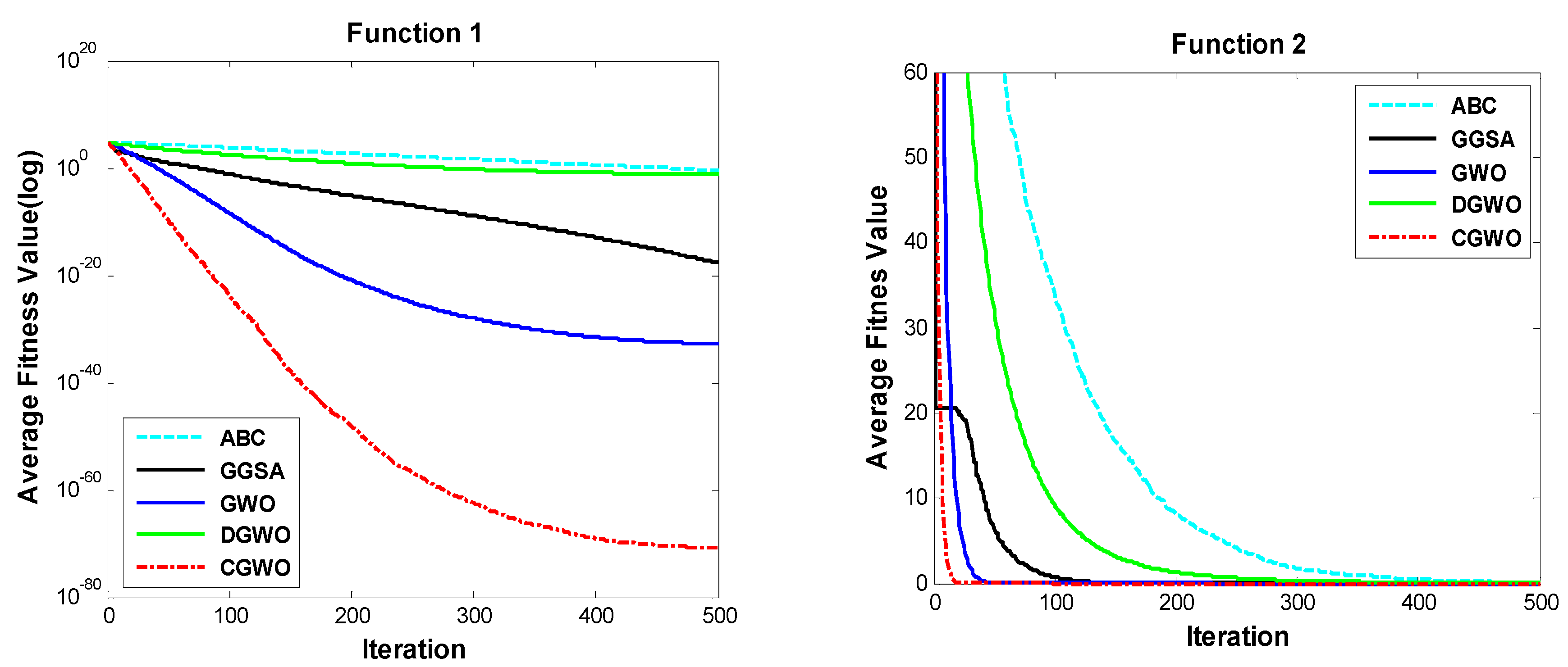
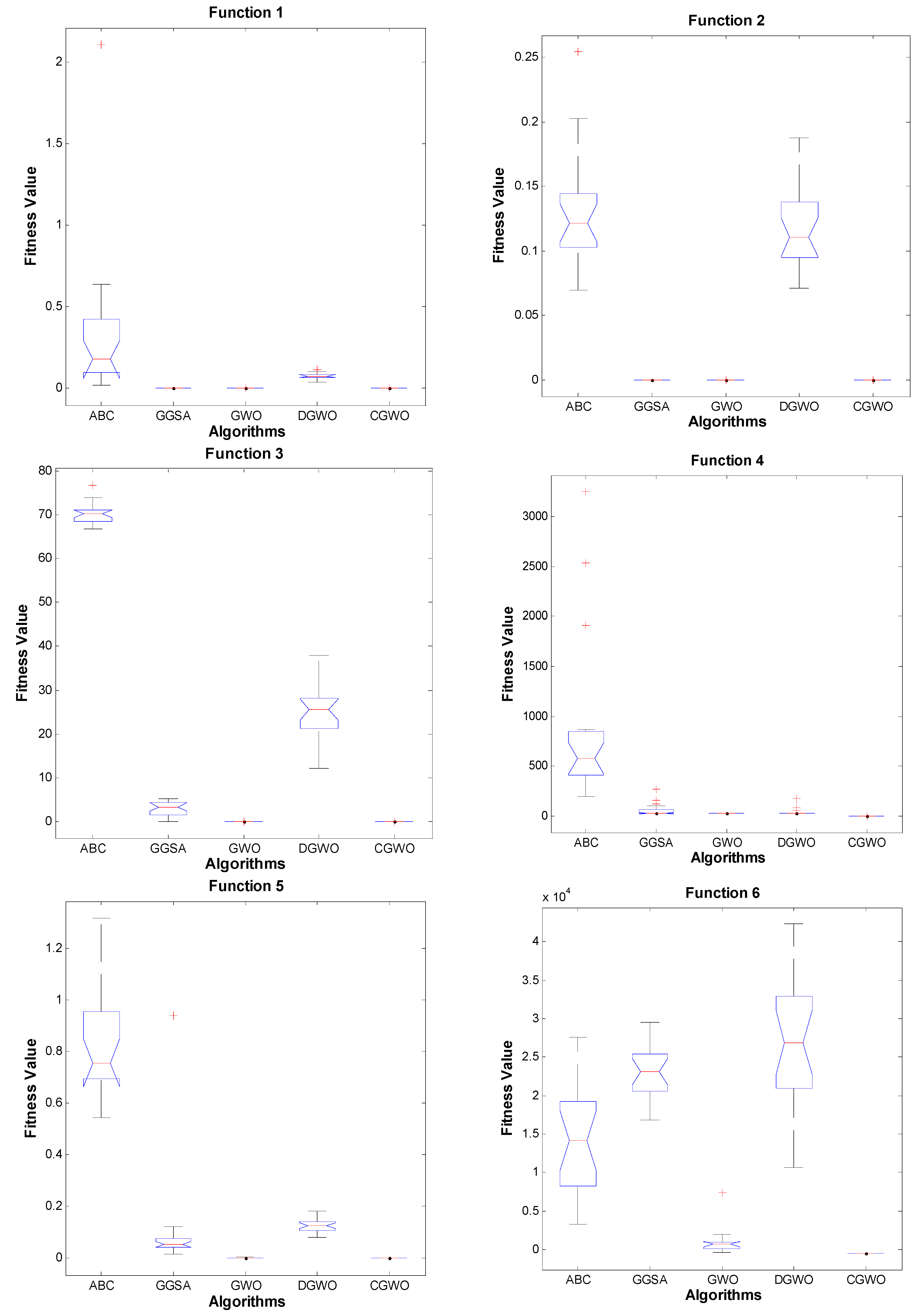
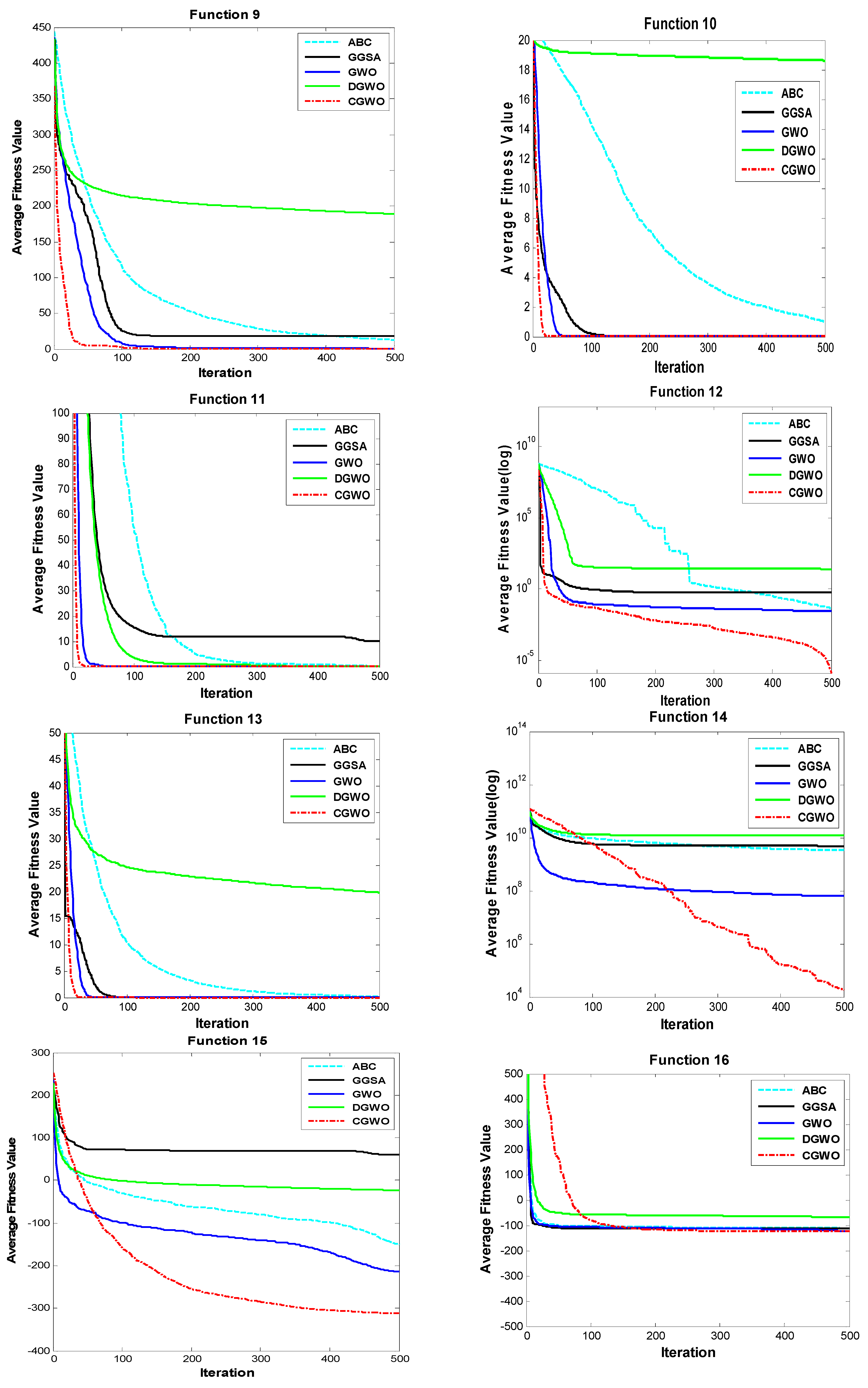
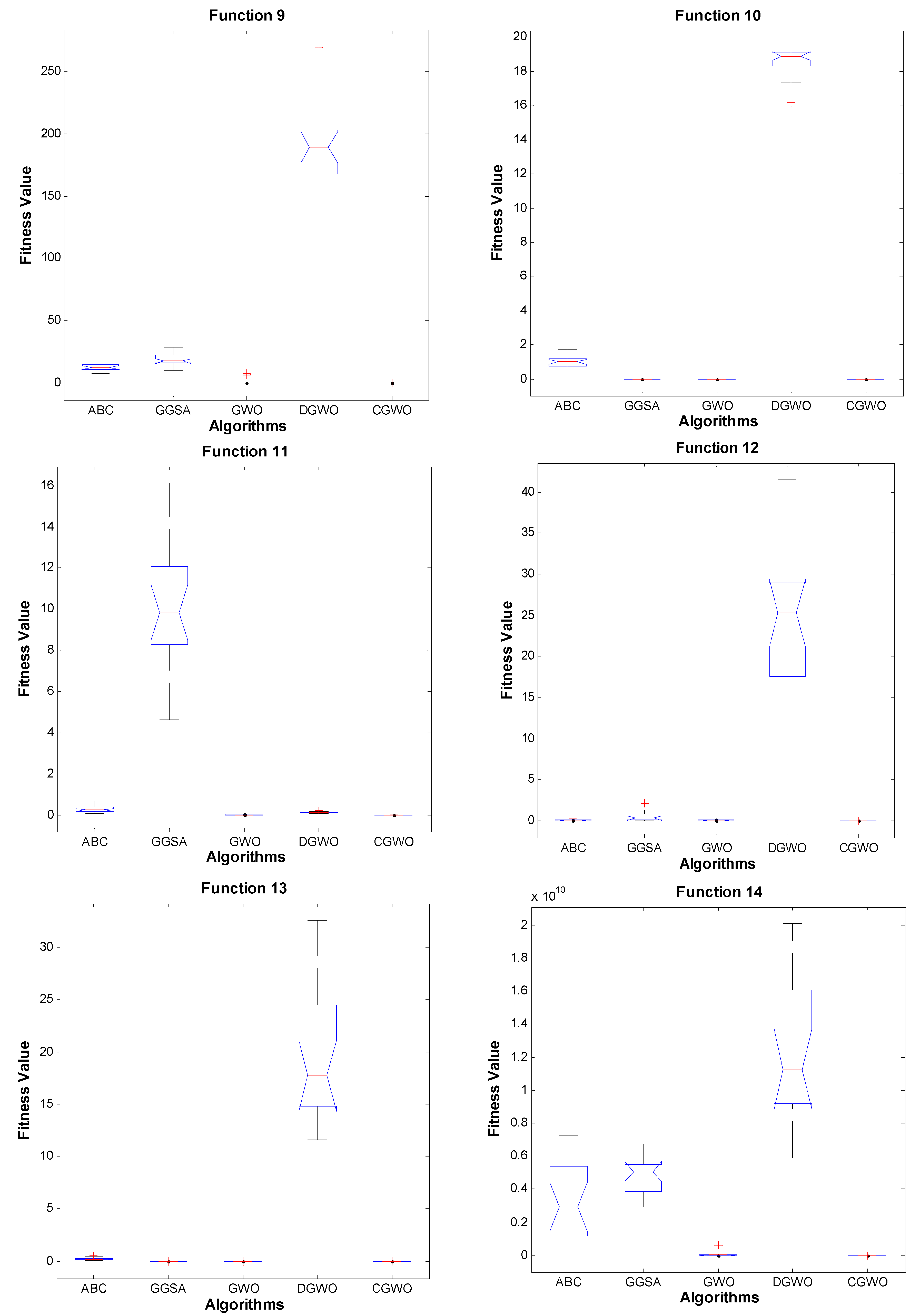
Figure 1 shows the averaged convergence curves of unimodal benchmark functions with 30-D over 20 independent runs. As shown from these curves, the CGWO has the fastest convergence rate. Figure 2 indicates the anova tests of the global minimum on unimodal functions with 30-D, which shows that CGWO is the most robust method. For functions, the other algorithms that we compared (namely, DGWO, GWO, GGSA, ABC) were only robust for a few functions and were not able to be robust for all functions. On the basis of Table 3, Table 5, Table 6, Table 7, Table 8, Table 9, Table 10 and Table 11 and Figure 1 and Figure 3, it can be concluded that the CGWO tends to find the best solution in unimodal functions with a very fast convergence rate and a more stable performance.
Figure 1.
Convergence behavior of ABC, GGSA, GWO, DGWO, and CGWO on unimodal functions with Dim = 30.
Figure 1.
Convergence behavior of ABC, GGSA, GWO, DGWO, and CGWO on unimodal functions with Dim = 30.


Figure 2.
ANOVA tests of ABC, GGSA, GWO, DGWO, and CGWO on unimodal functions with Dim = 30.


4.4. Multimodal Benchmark Functions
The results of the multimodal benchmark functions are provided in Table 4. Note that multimodal functions have many local minima with the number increasing exponentially with dimension. Therefore, they are very suitable to test the exploration capability of algorithms to avoid local minima. As the results of the mean and STD show, CGWO performs better than the other algorithms on 30-D, 50-D multimodal benchmark functions. For on 200-D, 300-D, 400-D, the GWO has better value than the CGWO. For on 10-D, the GGSA has best result. For on 100-D, the GWO is slightly better than the CGWO. For on 100-D, CGWO and GGSA have very close results. This table also shows that CGWO provides better results than the other algorithms across the majority of dimensions on 10-D, 100-D, 200-D, 300-D, and 400-D. Moreover, the p values of with different dimensions reported in Table 5, Table 6, Table 7, Table 8, Table 9, Table 10 and Table 11 are less than 0.05 across the majority of dimensions, which is strong evidence against null hypothesis. So, this evidence demonstrates that the results of CGWO are statistically significant and do not occur by coincidence.
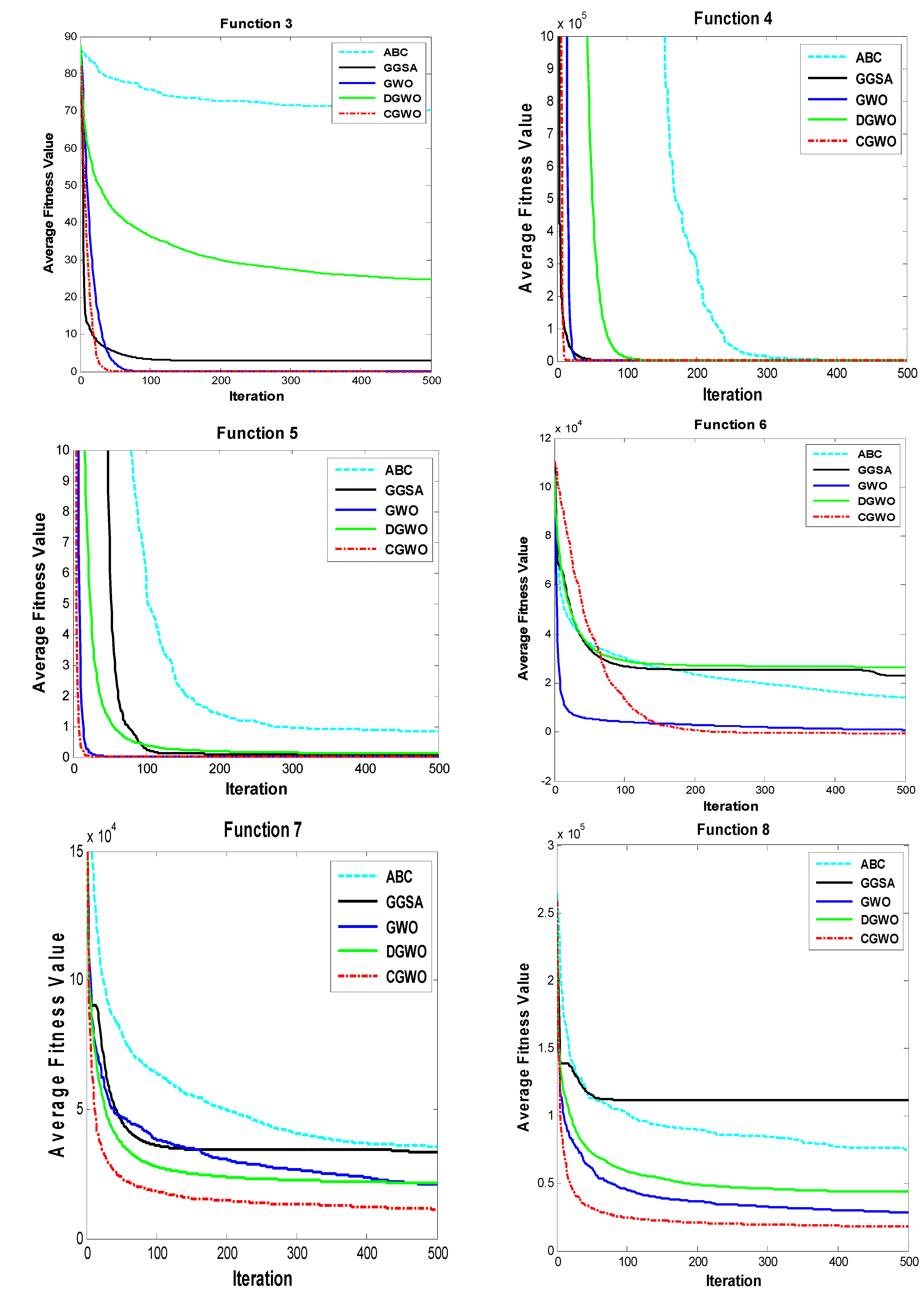
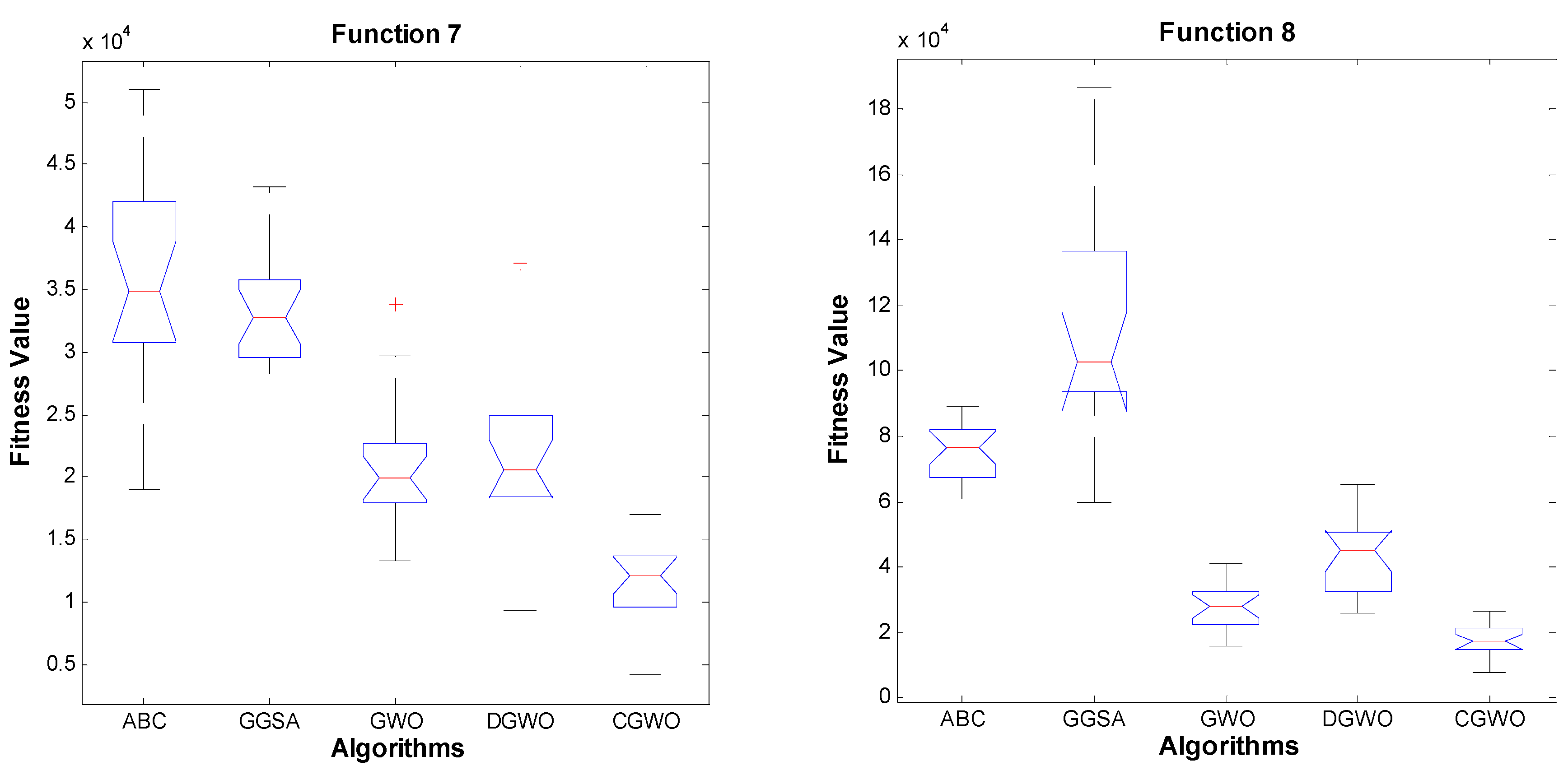
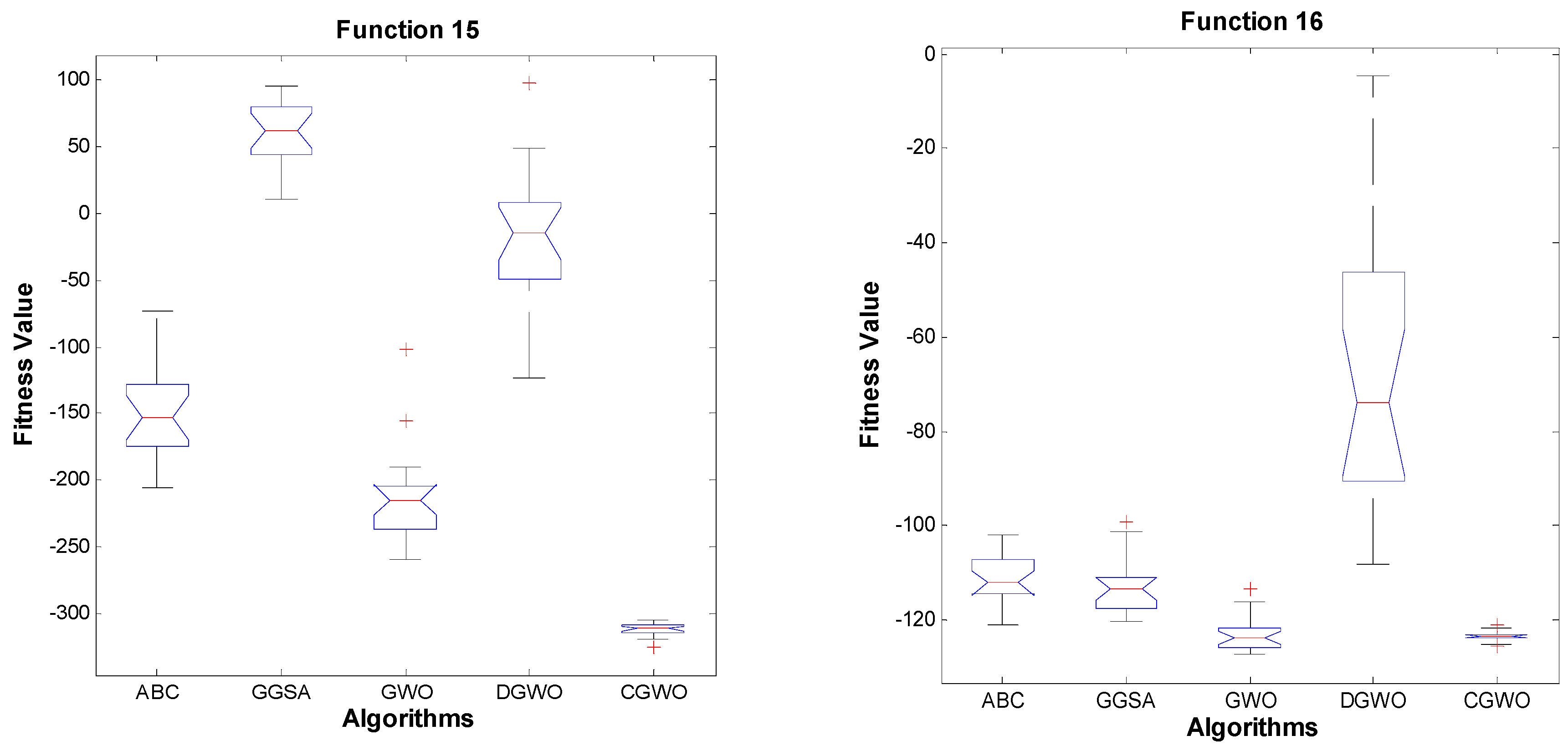
Figure 3 shows the averaged convergence curves of multimodal benchmark functions with 30-D over 20 independent runs. As shown in Figure 2, the convergence rate of CGWO in all cases is better than the other algorithms. Figure 4 depicts the anova tests between CGWO and the other algorithms on multimodal functions with 30-D. As shown, the more stable performance belongs to CGWO. According to Table 4, Table 5, Table 6, Table 7, Table 8, Table 9, Table 10 and Table 11 and Figure 3 and Figure 4, it can be stated that CGWO is capable of avoiding local minima with good convergence speed and stable property when dealing with multimodal benchmark functions.
According to this comprehensive comparative study and discussion, we state that this algorithm has merit compared to the other algorithms. The next section inspects the performance of the CGWO in solving the IIR model identification problem.
Figure 3.
Convergence behavior of ABC, GGSA, GWO, DGWO, and CGWO on multimodal functions with Dim = 30.
Figure 3.
Convergence behavior of ABC, GGSA, GWO, DGWO, and CGWO on multimodal functions with Dim = 30.

Figure 4.
ANOVA tests of ABC, GGSA, GWO, DGWO, and CGWO on multimodal functions with Dim = 30.


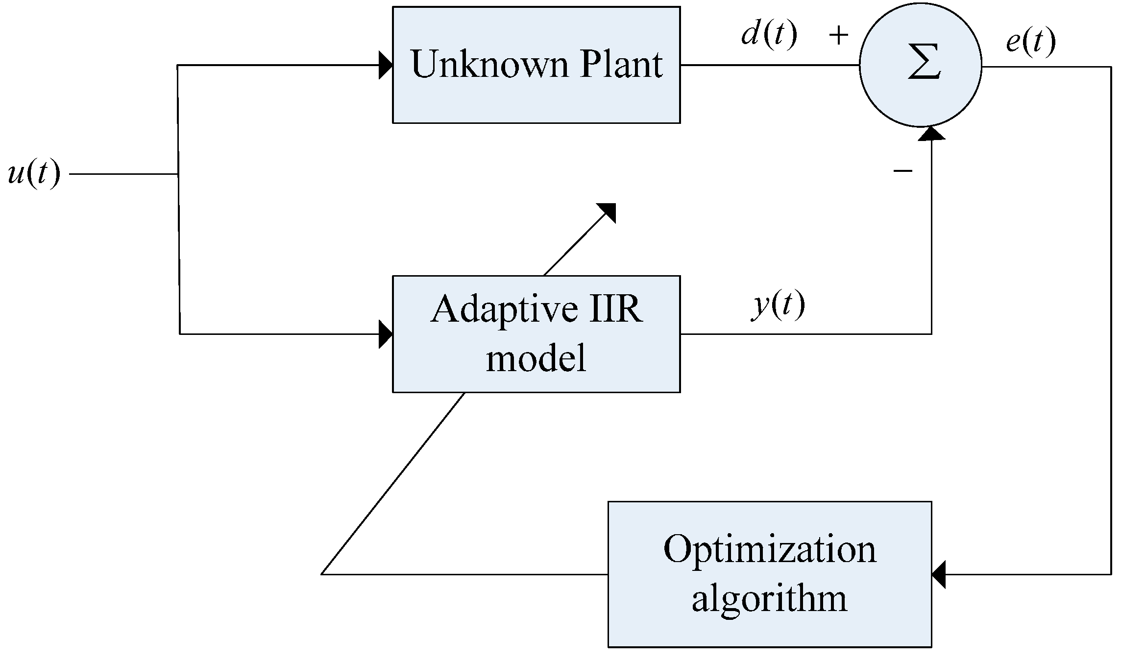
5. IIR Model Identification
System identification is an effective method to obtain the mathematical model of an unknown system by analyzing its input and output values. In system identification, the use of infinite impulse response (IIR) has been widely studied since many problems encountered in signal processing can be characterized as a system identification problem (Figure 5). In this case, an optimization algorithm tries to iteratively adjust the parameters until the error between the output of the candidate model and the actual output of the plant is minimized. The use of IIR models for identification is preferred over their equivalent FIR (finite impulse response) models since the former produce more accurate models of physical plants for real world applications [32]. Moreover, IIR models are able to use fewer model parameters to meet the performance specifications. The fitness function, which is used in the article, is calculated as follows [33].
Figure 5.
Block diagram of IIR system identification.

In an IIR system, the transfer function is provided as follows:
where and are the number of numerator and denominator coefficients of the transfer function, respectively, is the pole of the IIR model, is the zero parameters of the IIR model. Equation (17) is expressed in another form as follows:
where indicates the tth input of the system, indicates the tth output of the system. Hence, the set of unknown parameters that simulates the IIR system is indicated by . The number of unknown parameters of is . Correspondingly, the search space of IIR feasible values for is .
According to Figure 5, the output of the plant is , while the output of the IIR filter is . The error indicates the difference between the actual system and its model yields. Here the error is . Therefore, the problem of IIR model identification can be solved as a minimization problem of function. Additionally, the function can be molded as follows:
where indicates the number of the samples used in the simulation, and the aim is to minimize the function through adjusting . When the error function reaches its minimum value, the optimal model or solution is obtained. The is shown as follows:
IIR Model Identification Result
The result is reported considering a superior-order plant through a high-order IIR model. The unknown plant and the IIR model hold the following transfer function [27]:
Since the plant is a sixth-order system and the IIR model a fourth-order system, the error surface is multimodal. A white sequence with 100 samples has been used as input. The result of the experience over 20 consecutive experiments is shown in Table 5 and Table 6. Table 13 shows the best parameter values (ABP). Table 14 indicates the average value (AVE) and the standard deviation (STD). Figure 6 provides a comparison between CGWO and the other algorithms for IIR system identification.
| Algorithms | |||||||||
|---|---|---|---|---|---|---|---|---|---|
| CGWO | 1.1093E−02 | −4.9144E−01 | −2.9101E−03 | −3.3551E−01 | 9.8932E−01 | 1.3089E−02 | −1.2463E−01 | −1.5870E−02 | −7.3745E−02 |
| DGWO | 1.2382E−01 | 5.5593E−02 | −4.9268E−04 | 1.0155E−01 | 2.1844E−01 | −1.6315E−01 | −8.9793E−02 | −1.1818E−01 | 6.1028E−02 |
| GWO | −2.8883E−02 | −2.6764E−01 | −2.3851E−02 | −2.4399E−01 | 9.1861E−01 | −2.9241E−03 | 4.8354E−02 | −2.7404E−02 | 4.9129E−02 |
| GGSA | 4.6698E−01 | −1.1299E−01 | 5.7827E−02 | 1.8673E−01 | −3.6432E−02 | 1.0900E−01 | −8.4527E−02 | −8.4070E−02 | 3.0088E−01 |
| ABC | 9.9479E−03 | 4.4119E−02 | 5.9096E−02 | −2.2442E−01 | 8.3829E−01 | −1.1020E−01 | 2.8357E−01 | −4.1144E−02 | 1.1184E−01 |
| Algorithms | AVE | STD |
|---|---|---|
| CGWO | 3.4013E−03 | 2.1644E−03 |
| DGWO | 1.2513E−01 | 7.1059E−02 |
| GWO | 5.5317E−03 | 4.9962E−03 |
| GGSA | 1.2537E−02 | 2.4702E−03 |
| ABC | 4.7898E−02 | 1.2004E−02 |
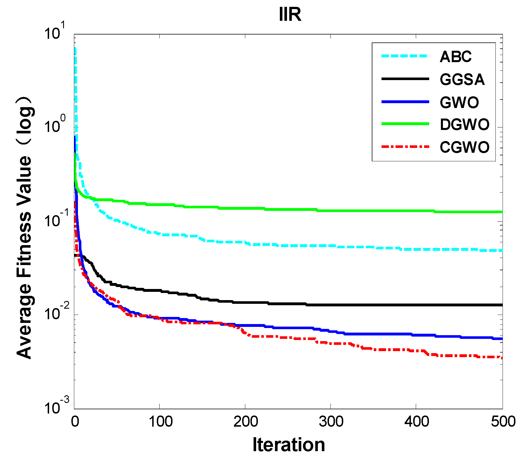
Figure 6.
Comparison between CGWO and the other algorithms for IIR system identification.

According to the AVE and STD indexes in Table 6, the CGWO algorithm finds better results than the other algorithms. The results show that CGWO provides better precision (AVE value) and robustness (STD). As shown in Figure 6, the CGWO has the fastest convergence rate.
In conclusion, the results show that the proposed method successfully outperforms the other algorithms in a majority of benchmark functions. In addition, IIR model identification shows that CGWO is able to obtain very competitive results. Therefore, as shown in the results of this comparative study, the proposed method has merit in the field of evolutionary algorithms and optimization.
6. Conclusions
In this work, the idea of complex-valued encoding is introduced into GWO, and a complex-valued version of GWO called CGWO was proposed based on complex-valued encoding. The proposed functions justified its excellent property on 16 benchmark functions in terms of improved avoidance of local minima and increased convergence speed. Furthermore, a complex system identification problem been employed to test the performance of the proposed method. The results verified the superior performance of CGWO on IIR model identification when compared to the other algorithms because of its improved ability. For future studies, it is recommended to apply the CGWO to solve more real-world engineering problems.
Acknowledgments
This work is supported by National Science Foundation of China under Grants No. 61463007; 6153008. Project of Guangxi University for Nationalities Science Foundation under Grant No. 2012MDZD037.
Author Contributions
Qifang Luo designed algorithm; Sen Zhang and Zhiming Li performed the experiments; Yongquan Zhou wrote the paper.
Conflicts of Interest
The authors declare no conflict of interest.
References
- Kennedy, J.; Eberhart, R. Particle swarm optimization. In Proceedings of the IEEE International Conference on Neural Networks, Perth, WA, USA, 27 November–1 December 1995; pp. 1942–1948.
- Holland, J.H. Genetic algorithms. Sci. Am. 1992, 267, 66–72. [Google Scholar] [CrossRef]
- Price, K.; Storn, R. Differential evolution. Dr. Dobb’s J. 1997, 22, 18–20. [Google Scholar]
- Price, K.V.; Storn, R.M.; Lampinen, J.A. Differential Evolution: A Practical Approach to Global Optimization; Springer: New York, NY, USA, 2005. [Google Scholar]
- Kirkpatrick, S.; Gelati, C.D.; Vecchi, M.P. Optimization by simulated annealing. Science 1983, 220, 671–680. [Google Scholar] [CrossRef] [PubMed]
- Dorigo, M.; Maniezzo, V.; Colorni, A. The ant system: Optimization by a colony of cooperating agents. IEEE Trans. Syst. Man Cybern. B 1996, 26, 29–41. [Google Scholar] [CrossRef] [PubMed]
- Karaboga, D.; Basturk, B. A powerful and efficient algorithm for numerical function optimization: Artificial bee colony (ABC) algorithm. J. Glob. Optim. 2007, 39, 459–471. [Google Scholar] [CrossRef]
- Rashedi, E.; Nezamabadi-Pour, H.; Saryazdi, S. GSA: A gravitational search algorithm. Inf. Sci. 2009, 179, 2232–2248. [Google Scholar] [CrossRef]
- Mirjalili, S.; Lewis, A. Adaptive gbest-guided gravitational search algorithm. Neural Comput. Appl. 2014, 25, 1569–1584. [Google Scholar] [CrossRef]
- Kaveh, A.; Talatahari, S. A novel heuristic optimization method: Charged system search. Acta Mech. 2010, 213, 267–289. [Google Scholar] [CrossRef]
- Tayarani, N.M.H.; Akbarzadeh, T.M.R. Magnetic optimization algorithms a new synthesis. In Proceedings of the IEEE Congress on Evolutionary Computation, Hong Kong, China, 1–6 June 2008; pp. 2659–2664.
- Simon, D. Biogeography-based optimization. IEEE Trans. Evol. Comput. 2008, 12, 702–713. [Google Scholar] [CrossRef]
- Mirjalili, S.; Mirjalili, S.M.; Lewis, A. Let a biogeographybased optimizer train your multi-layer perceptron. Inf. Sci. 2014, 269, 188–209. [Google Scholar] [CrossRef]
- Rao, R.V.; Savsani, V.J.; Vakharia, D.P. Teaching–learning-based optimization: A novelmethod for constrained mechanical design optimization problems. Comput.-Aided Des. 2011, 43, 303–315. [Google Scholar] [CrossRef]
- Wolpert, D.H.; Macready, W.G. No free lunch theorems for optimization. IEEE Trans. Evol. Comput. 1997, 1, 67–82. [Google Scholar] [CrossRef]
- Mirjalili, S.; Mirjalili, S.M.; Lewis, A. Grey wolf optimizer. Adv. Eng. Softw. 2014, 69, 46–61. [Google Scholar] [CrossRef]
- Sulaiman, M.H.; Mustaffa, Z.; Mohamed, M.R.; Aliman, O. Using the gray wolf optimizer for solving optimal reactive power dispatch problem. Appl. Soft Comput. 2015, 32, 286–292. [Google Scholar] [CrossRef]
- Song, X.H.; Tang, L.; Zhao, S.T.; Zhang, X.Q.; Li, L.; Huang, J.Q.; Cai, W. Grey Wolf Optimizer for parameter estimation in surface waves. Soil Dyn. Earthq. Eng. 2015, 75, 147–157. [Google Scholar] [CrossRef]
- Komaki, G.M.; Kayvanfar, V. Grey Wolf Optimizer algorithm for the two-stage assembly flow shop scheduling problem with release time. J. Comput. Sci. 2015, 8, 109–120. [Google Scholar] [CrossRef]
- Casasent, D.; Natarajan, S. A classifier neural network with complex-valued weights and square-law nonlinearities. Neural Netw. 1995, 8, 989–998. [Google Scholar] [CrossRef]
- Chen, D.-B.; Li, H.-J.; Li, Z. Particle swarm optimization based on complex-valued encoding and application in function optimization. Comput. Eng. Appl. 2009, 45, 59–61. [Google Scholar]
- Das, S.; Suganthan, P.N. Differential evolution: A survey of the state-of-the-art. IEEE Trans. Evol. Comput. 2011, 15, 4–31. [Google Scholar] [CrossRef]
- Yang, X.S. Appendix a: Test problems in optimization. In Engineering Optimization; Yang, X.S., Ed.; John: Hoboken, NJ, USA, 2010; pp. 261–266. [Google Scholar]
- Tang, K.; Yao, X.; Suganthan, P.N.; MacNish, C.; Chen, Y.P.; Chen, C.M.; Yang, Z. Benchmark Functions for the CEC’2008 Special Session and Competition on Large Scale Global Optimization; Technical Report; Nature Inspired Computation and Applications Laboratory, University of Science and Technology of China: Hefei, China, 2007; pp. 153–177. [Google Scholar]
- Suganthan, P.N.; Hansen, N.; Liang, J.J.; Deb, K.; Chen, Y.; Auger, A.; Tiwari, S. Problem Definitions and Evaluation Criteria for the CEC 2005 Special Session on Real-Parameter Optimization; Technical Report; Nanyang Technological University: Singapore, 2005; Volume 2005005. [Google Scholar]
- The Matlab Code of the GGSA Algorithm. Available online: http://www.alimirjalili.com/Projects.html (accessed on 10 October 2014).
- Derrac, J.; García, S.; Molina, D.; Herrera, F. A practical tutorial on the use of nonparametric statistical tests as a methodology for comparing evolutionary and swarm intelligence algorithms. Swarm Evol. Comput. 2011, 1, 3–18. [Google Scholar] [CrossRef]
- White, M.S.; Flockton, S.J. Adaptive recursive filtering using evolutionary algorithms. In Evolutionary Algorithms in Engineering Applications; Dasgupta, D., Michalewicz, Z., Eds.; Springer: Berlin, Germany, 1997; pp. 361–376. [Google Scholar]
- García, S.; Molina, D.; Lozano, M.; Herrera, F. A study on the use of non-parametric tests for analyzing the evolutionary algorithms’ behaviour: A case study on the CEC’2005 special session on real parameter optimization. J. Heuristics 2009, 15, 617–644. [Google Scholar] [CrossRef]
- Wilcoxon, F. Individual Comparisons by Ranking Methods; Biometrics Bulletin; International Biometric Society: Washington, DC, USA, 1945; pp. 80–83. [Google Scholar]
- Alcalá-Fdez, J.; Sánchez, L.; García, S.; del Jesus, M.J.; Ventura, S.; Garrell, J.M.; Otero, J.; Romero, C.; Bacardit, J.; Rivas, V.M.; et al. KEEL: A Software Tool to Assess Evolutionary Algorithms to Data Mining Problems. Soft Comput. 2009, 13, 307–318. [Google Scholar] [CrossRef]
- Kukrer, O. Analysis of the dynamics of a memoryless nonlinear gradient IIR adaptive notch filter. Signal Process. 2011, 91, 2379–2394. [Google Scholar] [CrossRef]
- Cuevas, E.; Gálvez, J.; Hinojosa, S.; Avalos, O.; Zaldívar, D.; Pérez-Cisneros, M. A Comparison of Evolutionary Computation Techniques for IIR Model Identification. J. Appl. Math. 2014, 2014, 768516. [Google Scholar] [CrossRef]
© 2015 by the authors; licensee MDPI, Basel, Switzerland. This article is an open access article distributed under the terms and conditions of the Creative Commons by Attribution (CC-BY) license (http://creativecommons.org/licenses/by/4.0/).
Share and Cite
MDPI and ACS Style
Luo, Q.; Zhang, S.; Li, Z.; Zhou, Y. A Novel Complex-Valued Encoding Grey Wolf Optimization Algorithm. Algorithms 2016, 9, 4. https://doi.org/10.3390/a9010004
AMA Style
Luo Q, Zhang S, Li Z, Zhou Y. A Novel Complex-Valued Encoding Grey Wolf Optimization Algorithm. Algorithms. 2016; 9(1):4. https://doi.org/10.3390/a9010004
Chicago/Turabian StyleLuo, Qifang, Sen Zhang, Zhiming Li, and Yongquan Zhou. 2016. "A Novel Complex-Valued Encoding Grey Wolf Optimization Algorithm" Algorithms 9, no. 1: 4. https://doi.org/10.3390/a9010004
Note that from the first issue of 2016, this journal uses article numbers instead of page numbers. See further details here.