Faster Force-Directed Graph Drawing with the Well-Separated Pair Decomposition ^†

Abstract

The force-directed paradigm is one of the few generic approaches to drawing graphs. Since force-directed algorithms can be extended easily, they are used frequently. Most of these algorithms are, however, quite slow on large graphs, as they compute a quadratic number of forces in each iteration. We give a new algorithm that takes only $O(m+nlogn)$ time per iteration when laying out a graph with n vertices and m edges. Our algorithm approximates the true forces using the so-called well-separated pair decomposition. We perform experiments on a large number of graphs and show that we can strongly reduce the runtime, even on graphs with less than a hundred vertices, without a significant influence on the quality of the drawings (in terms of the number of crossings and deviation in edge lengths).

1. Introduction

Force-directed algorithms are commonly used to draw graphs. They can be used on a wide range of graphs without further knowledge of the graphs’ structure. The idea is to define physical forces between the vertices of the graph. These forces are applied to the vertices iteratively until stable positions are reached. The well-known spring-embedder algorithm of Eades [1] models the edges as springs. His approach was refined by Fruchterman and Reingold [2]. Between pairs of adjacent vertices, they apply attracting forces caused by springs. These forces should cause the edge length to be as uniform as possible. To prevent vertices getting too close, they apply repulsive forces between all pairs of vertices.

Generally, force-directed methods are easy to implement and can be extended well. For example, Fink et al. [3] defined additional forces to draw Metro lines in Metro maps as Bézier curves instead of polygonal chains. Different aesthetic criteria can be balanced by weighing them accordingly. Force-directed algorithms can in principle be used for relatively large graphs with hundreds of vertices and often yield acceptable results. Unfortunately, force-directed methods are rather slow on such graphs. This is caused by the computation of the repulsive force for every vertex pair, which yields a quadratic runtime for each iteration. In this paper, we present a new approach to speed this up.

1.1. Previous Work

Many techniques for speeding up force-directed algorithms have been suggested. For example, Barnes and Hut [4] used a quadtree, a multi-purpose spatial data structure, to approximate the forces between the vertex pairs. We will compare our algorithm to theirs subsequently. Another approach is the multilevel paradigm introduced by Walshaw [5]. After contracting dense subgraphs, the resulting coarse graph is laid out. Then, the vertices are uncontracted, and the layout of the whole graph based on the coarse layout is computed. This can be done over several levels. The multilevel approach does not only speed up the computation, but also yields significantly better results in many cases where the corresponding single-level algorithm does not manage to “unfold” the given graph [5]. The multilevel paradigm does not rule out our speed-up technique; our technique can be applied to each individual level. We will exploit this in our experiments.

Hachul and Jünger [6] took the so-called fast multipole method from physics [7] to graph drawing, which is a method that helps to approximate the potentials in an n-body system by evaluating truncated Laurent series for pairs of clusters. The clustering is derived from a (reduced) quadtree. Hachul and Jünger also presented a new multilevel approach (based on partitioning the nodes into suns, planets and moons). Combining the two techniques, they managed to draw graphs of up to 100,000 vertices within a few minutes. Note, however, that the fast multipole method depends on repulsive forces whose decay is inversely proportional to the inter-node distance, that is for any two vertices u and v, the force that u exerts on v is $F_{\text{repulsive}}(u,v)=c/d(u,v)$, where c is a constant. The reason for the restriction is that this definition of the repulsive forces corresponds to a potential energy that is proportional to $-logd(u,v)$. Using the expansion of the complex logarithm, the potential energy can be approximated. Finally, the derivative of the (complex) potential energy function in a given point yields the repulsive force in that point; see Hachul’s thesis ([8], Lemmas 5.15 and 5.16 on page 104).

Later, Godiyal et al. [9] used a kd-tree to speed up the fast multipole method. In their implementation, they additionally used parallelization on a GPU, which sped up the algorithm significantly. Various force-directed graph drawing algorithms have been compared by experimental evaluations before [10,11,12]. We use two of the quality criteria described in the literature to evaluate our algorithm: the number of edge crossings and the standard deviation of the edge length.

Callahan and Kosaraju [13] defined a decomposition for point sets in the plane, the Well-Separated Pair Decomposition (WSPD). Given a point set P and a number $s>0$, this decomposition consists of pairs of subsets ${(A_i,B_i)}_{i=1,\dots ,k}$ of P with two properties. First, for each pair $(p,q)\in P^2$ with $p\ne q$, there is a unique index $i\in \{1,\dots ,k\}$, such that $p\in A_i$ and $q\in B_i$ or vice versa. Second, each pair $(A_i,B_i)$ must be s-well-separated, that is the distance between the two sets is at least s-times the larger of the diameters of the sets. Callahan and Kosaraju showed how to construct a WSPD for a set of n points in two dimensions in $O(n(logn+s^2))$ time where the number k of pairs of sets is in $O(s^{2}n)$.

The WSPD has been used for graph drawing before; Gronemann [14] employed it to speed up the fast multipole multilevel method [6] on multicore and single-instruction multiple-data (SIMD) architectures. While our WSPD is based on the split tree [13], Gronemann’s is based on a reduced quadtree. His implementation assumes that points are located on an integer grid, but the grid size can be very large, for example, $2^{32}\times 2^{32}$. He exploits the fact that, in this case, the bit representation of the integer coordinates can be used for constructing the quadtree bottom-up. For a fixed grid size, the algorithm runs in $O(nlogn)$ time, but the runtime depends on the distribution of the points. It assumes that the number of points sharing the same grid position is constant; otherwise, the running time deteriorates.

Huang et al. [15] use more forces to improve additional aesthetic criteria of the resulting drawing. They use so-called cosine forces to increase the size of crossing angles and sine forces to improve the angular resolution of vertices. They conducted a user study that shows that an algorithm adhering to these additional aesthetic criteria produces better graph drawings. Lin and Yen [16] extend Eades’ classical algorithm [1] by introducing repulsive forces between pairs of neighboring edges. With this approach, they want to increase the angular resolution; in particular, they want to avoid that edges incident to a common vertex overlap. Their evaluation of the algorithm indicates that the resulting drawings preserve the original properties and that all vertices have positive angular resolution. Additionally, they claim that the generated drawings usually have larger average angular resolution than drawings generated by the classical algorithm.

1.2. Our Contribution

We use the WSPD in order to speed up the force-directed algorithm of Fruchterman and Reingold (FR). Instead of computing the repulsive forces for every pair of points, we represent every set $A_1,\dots ,A_k,B_1,\dots ,B_k$ in the decomposition by its barycenter and use the barycenter of a set, say $A_i$, as an approximation when computing the forces between this set and a point in $B_i$. For laying out a graph with n vertices and m edges, the resulting runtime is $O(m+nlogn)$ per iteration, instead of $\mathrm{\Omega }(n^2)$ for the classical algorithm.

Our method is very simple and allows the user to define forces arbitrarily, as long as the total force on a point p is the sum of the forces of point pairs in which p is involved. Hence, our approach can be applied to any algorithm whose force model fulfills this requirement, which holds for all force-directed methods of which we know. For example, Hu [17] suggests to define the repulsive forces as $F_{\text{repulsive}}(u,v)=c/d^p(u,v)$ for any $p>0$. In the sequel, he uses $p\in \{2,3\}$ for some graph classes such as trees, in order to reduce peripheral effects, but he also gives an example with $p=1.3$ ([17], Figure 14). We do not consider other techniques, such as multidimensional scaling (MDS), as we only want to show that we can speed up force-directed graph layout algorithms using the WSPD. Our method combines well with the multilevel approach.

In contrast to our WSPD-based implementation of FR, the above-mentioned fast multipole method uses an approximation of the repulsive forces that is quite complicated (as Hachul and Jünger [6] point out); it requires the expansion of a Laurent series. Furthermore, it is restricted to repulsive forces that decay inversely proportionally with the node–node distance. In contrast to the work of Godiyal et al. [9], our speed-up technique does not assume access to the GPU. Other than Gronemann [14], we do not round vertex positions to an integer grid, and our speed-up technique does not rely on certain types of hardware architectures.

We first detail how we use the WSPD to speed up FR; see Section 2. Then, we test our modified algorithm on six types of real-world and synthetic data sets. We compare several versions of FR in terms of running time and two commonly-used quality metrics (namely number of crossings and deviation of edge lengths); see Section 3.

Our algorithm is implemented in Java based on JUNG [18]. While this makes it difficult to compare running times to the algorithms implemented in C++ in the Open Graph Drawing Framework (OGDF [19]), we have found and fixed bugs in the only existing Java implementation of FR (in JUNG). Our speed-up technique will serve the Java community and will potentially popularize graph drawing methods in that community. The source code for our Java implementation and our test data sets can be found on our webpage [20].

2. Algorithm

In this section, we describe our WSPD-based implementation, analyze its asymptotic running time and give a heuristic speed-up method.

2.1. Constructing a WSPD

There are various ways to construct an efficient WSPD, that is a WSPD with a linear number of pairs of sets. We use the split tree as described by Callahan and Kosaraju [13] when introducing the WSPD. Our implementation follows the algorithm FastSplitTree in the textbook of Narasimhan and Smid ([21], Section 9.3.2). Given n points, this algorithm constructs a linear-size split tree in $O(nlogn)$ time. Given the tree, a WSPD with separation constant s can be built in $O(s^{2}n)$ time. To construct the WSPD, we traverse the split tree top-down. For each internal node α, we introduce well-separated pairs that separate the sets represented by the node’s two children β and ${\beta }^{\prime }$. Given the split tree nodes α, β and ${\beta }^{\prime }$, we denote the corresponding point sets by A, B and $B^{\prime }$. If the pair $(B,B^{\prime })$ is s-well-separated, we add it to the WSPD. Otherwise, suppose that the bounding box of B has larger area than that of $B^{\prime }$. In this case, we replace β by its two children and check whether the corresponding point sets form s-well-separated pairs with $B^{\prime }$. We continue this recursive process until the WSPD contains, for each pair of points $(p,p^{\prime })\in B\times B^{\prime }$, a unique s-well-separated pair that separates p and $p^{\prime }$. Narasimhan and Smid ([21], Section 9.4) show that this algorithm is correct and runs in $O(s^{2}n)$ time.

2.2. The Force-Directed Algorithm

The general principle of a force-directed algorithm is as follows. In every iteration, the algorithm computes forces on the vertices. These forces depend on the current position of the vertices in the drawing. The forces are applied as an offset to the position of each vertex. The algorithm terminates after a given number of iterations or when the forces get below a certain threshold.

A classical force-directed algorithm, such as FR, computes, in every iteration, an attractive force for any pair of adjacent vertices and a repulsive force for any pair of vertices. We follow Fruchterman and Reingold [2] and use forces $F_{\text{attractive}}(u,v)=d^2(u,v)/c$ and $F_{\text{repulsive}}(u,v)=-c^2/d(u,v)$, where c is a constant describing the ideal edge length and $d(u,v)$ is the distance between vertices u and v in the current drawing.

Our modified algorithm is shown in Algorithm 1. We do not modify the computation of the attractive forces. We first compute a fair split tree T for the current positions of the vertices of G (which are stored in the leaves of T). Each node μ of T corresponds to the set of vertices in the leaves of the subtree rooted at μ. We need to know the positions of the barycenters of the sets corresponding to the nodes of T to compute the values of the repulsive forces. Those can be computed in linear time by traversing the split tree bottom-up. We start with the leaves of the split tree, which only consist of one vertex. The barycenter of a one-element set is equal to the vertex position, of course. For the other nodes in the split tree, we can compute the barycenter as the weighted sum of the barycenters of its child nodes.

Algorithm 1: WSPD-Based Force Computation for a Graph $G=(V,E)$.

From T, we compute a WSPD ${(A_i,B_i)}_i$ for the current vertex positions. Each set $A_i$ (and $B_i$) of the WSPD corresponds to a node ${\alpha }_i$ (and ${\beta }_i$) of T. For each pair $(A_i,B_i)$ of the WSPD, we compute $F_{\text{repulsive}}$ from the barycenter of $A_i$ to the barycenter of $B_i$ (and vice versa) and store the results (in an accumulative fashion) in ${\alpha }_i$ and ${\beta }_i$. Finally, we traverse T top-down. During the traversal, we add to the force of each node the force of the parent node. When we reach the leaves of T, which correspond to the graph vertices, we have computed the resulting force for each vertex.

2.3. Running Time

We denote the number of vertices of the given graph by n and the number of edges by m. In each iteration, the classical algorithm computes the attractive forces in $O(m)$ time and the repulsive forces in $O(n^2)$ time.

As the classic algorithm, we compute the attractive forces in $O(m)$ time. For computing the repulsive forces, the most expensive step is the computation of the split tree T and the WSPD, which takes $O(nlogn)$ time. The barycenters of the sets corresponding to the nodes of T can be computed bottom-up in linear time. The forces between the pairs of the WSPD can also be computed in linear total time. The same holds for the forces acting on the vertices. Hence, in total, an iteration takes $O(m+nlogn)$ time.

2.4. Implementation

Our Java implementation is based on FRLayout, the FR algorithm implemented in the Java Universal Network/Graph Framework (JUNG, [18]). We slightly optimized the code, which reduced the runtime by a constant factor, and we removed the frame that was used to bound the drawing area, as it caused ugly drawings for larger graphs. If the graph is not connected, we now consider the connected components separately and draw them next to each other. Additionally, we changed the termination criterion for the loop, which now tests whether a predefined maximum number of iterations is reached or whether the movement of all vertices is below a certain threshold.

Further, we extended FRLayout with a multilevel approach that is based on the multilevel implementation in Gronemann’s FastMultipoleEmbedder in OGDF [19]. This particular multilevel approach uses Hachul’s galaxy partitioning [8], which was already mentioned in the Introduction, and can be used with any variant of FRLayout. For our experimental comparison in Section 3, we used FRLayout with these modifications. It is this implementation that we then sped up using the WSPD. We call the result FR+WSPD.

2.5. Improvements

To speed up our algorithm, we can compute a new split tree and the resulting WSPD only every few iterations. To be precise, we suggest to recompute these data structures only if $\lfloor 5logi\rfloor$ changes, where i is the index of the current iteration. Thus, the WSPD may not be valid for the current vertex positions. This makes the approximation of the forces more inaccurate, but our experiments show that this trick does not change the quality of the drawings significantly, whereas the running time decreases notably. Often, the number of edge crossings even decreases when the trick is used. An example is shown in Figure 1 for comparison. Nevertheless, we do not use this improvement in the following section to be more comparable to the other algorithms.

3. Experimental Comparison

We formulate the following hypotheses, which we then test experimentally.

(H1)

The quality of the drawings produced by FR+WSPD is comparable to that of FRLayout.

(H2)

On sufficiently large graphs, FR+WSPD is faster than FRLayout.

We assume these hypotheses due to the favorable properties of the WSPD: the separation property hints at (H1), and the improved time complexity per iteration implies (H2).

3.1. Experimental Setup

Apart from FRLayout and FR+WSPD, we implemented the quadtree-based speed-up method of Barnes and Hut [4], which we call FR+Quad, and a grid-based approach suggested already by Fruchterman and Reingold [2], which we call FR+Grid. To widen the scope of our study, we included some algorithms implemented in C++ in OGDF [19]: GEM (short for Graph Embedder) of Frick et al. [12], FM${}^3$ (short for Fast Multipole Multilevel Method) of Hachul and Jünger [6], the FastMultipoleMultilevelEmbedder of Gronemann (which is based on the idea of FM${}^3$ and Gronemann’s thesis [14]; we will call this variant simply FastMultipole), and FRExact (the exact FR implementation in OGDF; the corresponding class is called SpringEmbedderFRExact). We combine FRExact and GEM with MultilevelLayout in OGDF for our experiments. The other algorithms already include a multilevel implementation. Additionally, we use the ComponentSplitterLayout, as some OGDF algorithms can handle only connected graphs.

Our modified Java algorithms use the same termination criterion as FRExact. They are still, however, different in the implementation details (for example, the effect of the cooldown function), which leads to a different number of iterations when comparing the two implementations. Therefore, the relationships between the algorithms from JUNG and OGDF have to be interpreted with caution. In particular, the runtimes should not be compared in absolute numbers as the premises are very different for Java and C++.

We tested our algorithms on six data sets:

(DS1)

Rome: The Rome graph collection [23] contains 11,528 undirected connected graphs with 10–100 vertices each.

(DS2)

North: The North graphs [24], a subset of the AT&T graph collection, contain 1277 directed connected graphs with 10–100 vertices each. We only consider the underlying undirected graphs.

(DS3)

Rand-IncVtc-LoDens: A set of 40 random graphs that we generated using the class EppsteinPowerLawGenerator [25] in JUNG, which yields graphs whose structure is similar to web graphs. We generated instances with 2500, $5000,7500,\dots$, 100,000 vertices and approximately 2.5-times as many edges. We considered only the largest connected component of each generated graph, which contains most of the original vertices.

(DS4)

Rand-5000Vtc-IncDens: A set of 40 random graphs generated as (DS3). We fixed the number of vertices to 5000 and generated approximately $1,1.5,2,\dots ,20,20.5$-times as many edges to be able to test graphs with different densities. We considered only the largest connected component of each generated graph. This affected only the graphs with less than 25,000 edges.

(DS5)

Rand-1000Vtc-HiDens: A set of 40 random graphs generated as (DS3). We fixed the number of vertices to 1000 and the number of edges to approximately $10,000$. Each of these graphs is connected.

(DS6)

Hachul: The set of artificial graphs generated by Hachul and Jünger [22]. We use a subset of 45 graphs containing up to 10,000 vertices and up to 22,402 edges for our experiments. Some of these graphs are not connected.

The experiments were performed on an Intel Xeon CPU with 2.67 GHz and 16 GB RAM running Linux. The computer has 16 cores, but we did not parallelize our code. During our experiments, only one core was operating at close-to-full capacity.

We measured the quality of the drawings by (a) the number of edge crossings and (b) the standard deviation of the edge lengths (normalized by the mean edge length). These criteria have been used before to compare force-directed layout algorithms [11,12]. We did not measure our quality criteria on the large graphs—(DS3) and (DS4)—as the running time to count the number of edge crossings was too high in our naive implementation.

We first compared the outputs of FR+WSPD for different values ($0.0001$, $0.001$, $0.01$, $0.1$, 1 and 10) of the separation constant s on (DS1). The performance of the algorithm is shown in Figure 2. The distribution of the results in the plot is roughly the same, that is the quality of the drawings did not strongly depend on s. The runtimes for different values of s are shown in Figure 3. Using $s=10$ or $s=1$ was slower than the other values, so we found $s=0.1$ to be the best choice, which we use in the following experiments.

Similarly, FR+Quad has a parameter Θ that controls how finely the given point set is subdivided. Increasing Θ decreases the running time. Our experiments confirmed what Barnes and Hut [4] observed: only values of Θ close to one give results with a similar quality as the unmodified algorithm.

3.2. Results of Comparison

To test Hypothesis (H1), we compared the quality of the drawings produced by FRLayout and FR+WSPD for the data sets (DS1), (DS2), (DS5) and (DS6) using a statistical test. More precisely, we want to show that the number of crossings produced by our FR+WSPD algorithm is at most 10% worse, and the standard deviation of the edge lengths is at most 25% worse than the original FRLayout algorithm. To see this, we formulate the following null hypothesis: the number of crossings (resp., the standard deviation of the edge lengths) yielded by FR+WSPD is more than $1.1$-times (resp., $1.25$) the value yielded by FRLayout. It turned out that we can reject this null hypothesis using a Wilcoxon signed rank test [26] with high significance (p-values of $0.01$ at most).

Additionally, we compared the quality of the drawings produced by our FR+WSPD algorithm to that of other graph drawing algorithms. In order to vary as few parameters as possible, we kept the size of the graphs constant in this part of the study. We used all Rome graphs with exactly 100 vertices. The 140 graphs have, on average, 135 edges.

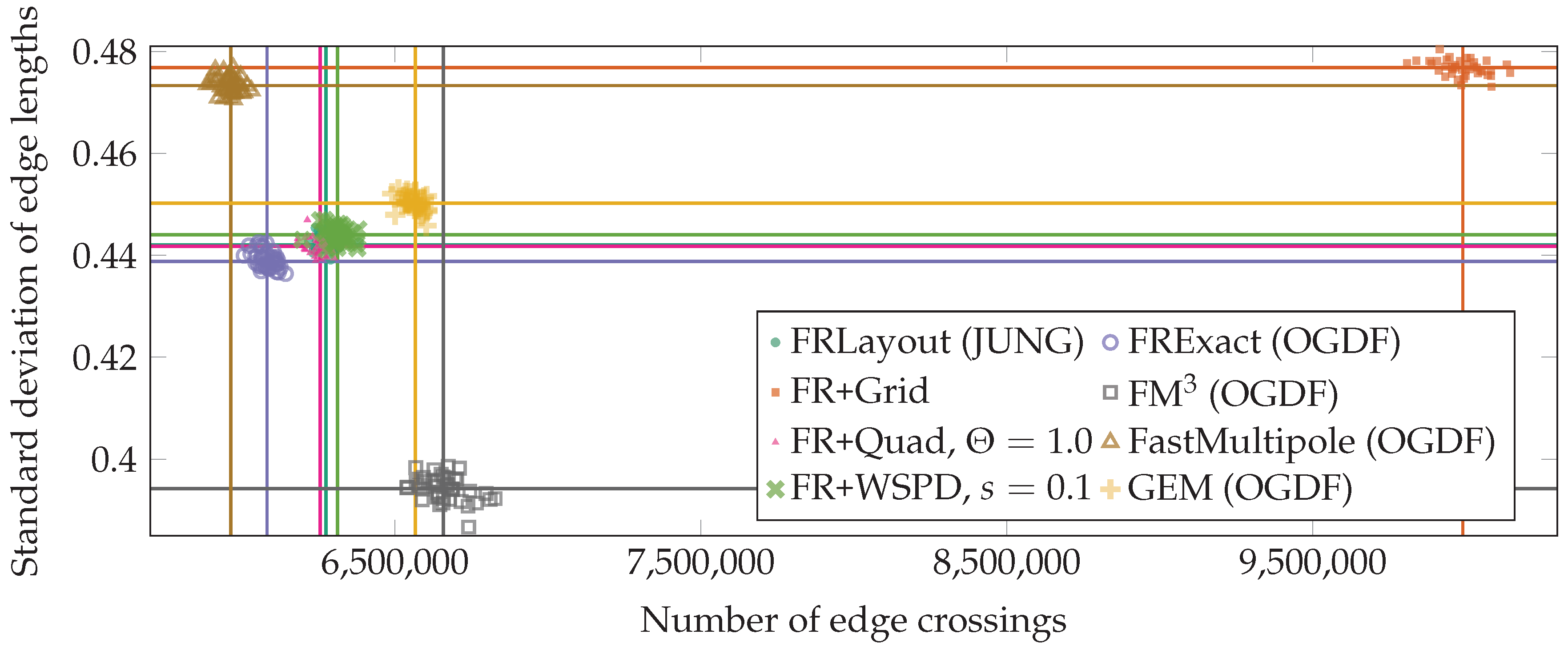
The lower scatterplot in Figure 4 compares FR+WSPD to the above-mentioned four OGDF algorithms. In terms of the uniformity of edge lengths, there are three clear clusters: FM${}^3$ is better and FastMultipole is worse than the rest (FRExact, GEM and FR+WSPD). In terms of crossings, however, FastMultipole is best, followed by GEM, FRExact, FM${}^3$ and FR+WSPD.

For the relatively dense graphs with 1000 vertices in Rand-1000Vtc-HiDens (DS5), Figure 5 shows a similar picture, except that here, FR+Grid is clearly the worst in both measures. FR+WSPD is in the mid-field according to both measures.

The upper scatterplot in Figure 4 compares the four variants of FR based on different speed-up techniques, which we have implemented in Java. In terms of the uniformity of edge lengths, FRLayout and FR+Quad are slightly better than FR+WSPD and FR+Grid. FR+Grid produces considerably more edge crossings than the other three variants. While FRLayout is somewhat better than FR+WSPD in both measures, there is support for Hypothesis (H1).

To test Hypothesis (H2), we measured the runtimes of all algorithms on our test data sets. Whenever an input graph was not connected, we measured the runtime for drawing all of its connected components. In Java, we only measure the time used for the thread running the force-directed algorithm in our Java Virtual Machine (using the method java.lang.management.ManagementFactory.get ThreadMXBean().getCurrentThreadCpuTime()); this eliminates the influence of the garbage collector and the JIT compiler on our measurements. In C++, we used the OGDF method ogdf::usedTime for measuring the CPU time. For each graph size, we display the mean runtime over all graphs of that size.

Figure 6 shows the runtimes for a test set with smaller graphs: Rome (DS1). The runtime curves for the North graphs were very similar to those of the Rome graphs, but due to the much smaller number of graphs, less smooth. Due to the similarity, we only show the plots for the Rome graphs. Figure 7 shows the runtimes for the test sets with larger graphs; (DS3), (DS4) and (DS5).

The results are as follows. As expected, FR+WSPD is much faster than FRLayout on larger graphs. We were surprised, however, to see that FR+WSPD starts overtaking FRLayout already around $n\approx 100$. For the Java variants, we could isolate the part of the running time that is used for the computation of the repulsive forces, which is the part we have improved and in which we are most interested; see Figure 6 and compare the top plot that shows the total running times to the bottom plot that shows the times needed for computing the repulsive forces. To show more details in the bottom plot, note that we used a different scale on the y-axis. The plot clearly shows that, as expected, computing the repulsive forces dominates the total running time.

On larger graphs, FR+WSPD turned out to be faster than all other algorithms in our comparison, except for FastMultipole for the very large, but low-density graphs in Rand-IncVtc-LoDens (DS3) and except for FR+Grid in the other two data sets (DS4) and (DS5). Recall, however, that FR+Grid tends to produce a much more edge crossings (Figure 5).

Concerning the comparison between Java and C++, FRExact (in C++) is roughly 2–3-times faster than FRLayout (in Java) for graphs of constant density; see Figure 5 (top and bottom). Increasing the number of edges slows FRLayout down much more than FRExact; see Figure 5 (middle). Of course, the comparison between different programming languages is not really fair because every language has its own advantages and disadvantages regarding efficiency. Still, our experiments show that the running times of FR+WSPD are in the same order of magnitude as those of OGDF.

The quality measures and runtimes for data set Hachul (DS6) are shown in Figure 8. We do not show absolute values for this data set, as the graphs are very different from each other and the differences in the results are hard to see in a properly-scaled plot. Instead, we rank the results from 1 (best)–8 (worst). The plots show that the quality depends on the instance: for many instances, FR+WSPD is quite good in terms of edge crossings, while it is often worse in terms of edge length deviation. In terms of running time, FR+WSPD is usually among the two or three fastest implementations in our comparison, regularly beaten only by FR+Grid (which produces many more edge crossings).

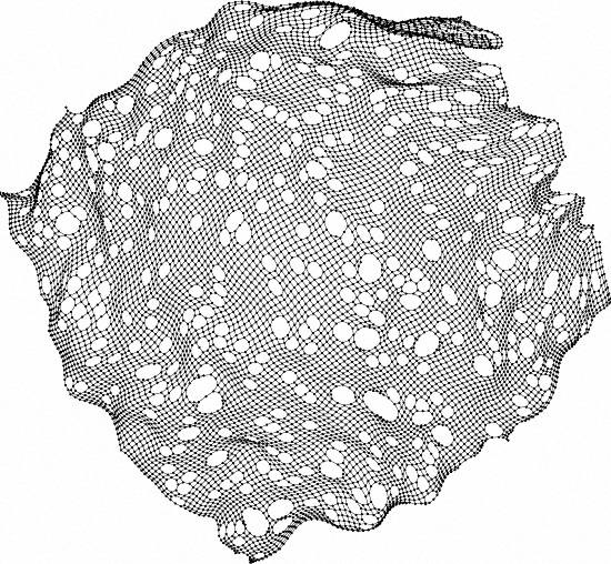
Figure 9, Figure 10 and Figure 11 show some example graphs drawn by six of the eight algorithms in our comparison. These artificial graphs were generated by Hachul and Jünger [22].

4. Conclusions and Perspectives

Our experiments show that the WSPD-based approach speeds up force-directed graph drawing algorithms, such as FR, considerably without noticeably sacrificing the quality of the drawing. The main feature of the new approach is its simplicity. We used the approach for the FR algorithm, but it can also be applied to other force-directed graph drawing algorithms and integrates well with multilevel approaches.

Compared to the other implementations in our comparison, the WSPD-based approach was among the fastest for graphs with more than 100 vertices; see Figure 7. With respect to quality, FR+WSPD was usually in the mid-range, somewhat better in terms of the number of crossings and slightly worse in terms of the standard deviation of edge lengths; see Figure 5 and Figure 8. Considering the specific examples that we picked from the Hachul data set ((DS6); see Figure 9, Figure 10 and Figure 11), Hachul and Jünger’s FM${}^3$ and (to a slightly lesser degree) Gronemann’s FastMultipole tend to yield the aesthetically most pleasing drawings. It would be interesting to understand better which part of the FM${}^3$ approach causes this difference.

There is still room for improvements. Could we, for example, quickly test whether it is necessary to recompute the WSPD? This decision has a strong impact on running time and quality. Instead of recomputing the WSPD, is there a way to update it dynamically as vertices move?

References

1. Eades, P. A heuristics for graph drawing. Congr. Numerantium 1984, 42, 146–160. [Google Scholar]
2. Fruchterman, T.M.J.; Reingold, E.M. Graph drawing by force-directed placement. Softw. Pract. Exp. 1991, 21, 1129–1164. [Google Scholar] [CrossRef]
3. Fink, M.; Haverkort, H.; Nöllenburg, M.; Roberts, M.; Schuhmann, J.; Wolff, A. Drawing Metro Maps Using Bézier Curves. In Graph Drawing; Springer: Heidelberg, Germany, 2013; pp. 463–474. [Google Scholar]
4. Barnes, J.; Hut, P. A hierarchical O(N log N) force-calculation algorithm. Nature 1986, 324, 446–449. [Google Scholar] [CrossRef]
5. Walshaw, C. A Multilevel Algorithm for Force-Directed Graph-Drawing. J. Graph Algorithms Appl. 2003, 7, 253–285. [Google Scholar] [CrossRef]
6. Hachul, S.; Jünger, M. Drawing large graphs with a potential-field-based multilevel algorithm. In Graph Drawing; Springer: Heidelberg, Germany, 2005; pp. 285–295. [Google Scholar]
7. Greengard, L.; Rokhlin, V. A fast algorithm for particle simulations. J. Comput. Phys. 1987, 73, 325–348. [Google Scholar] [CrossRef]
8. Hachul, S. A Potential-Field-Based Multilevel Algorithm for Drawing Large Graphs. Ph.D. Thesis, Universität zu Köln, Cologne, Germany, 2005. [Google Scholar]
9. Godiyal, A.; Hoberock, J.; Garland, M.; Hart, J.C. Rapid Multipole Graph Drawing on the GPU. In Graph Drawing; Springer: Heidelberg, Germany, 2009; pp. 90–101. [Google Scholar]
10. Bartel, G.; Gutwenger, C.; Klein, K.; Mutzel, P. An Experimental Evaluation of Multilevel Layout Methods. In Graph Drawing; Springer: Heidelberg, Germany, 2011; pp. 80–91. [Google Scholar]
11. Brandenburg, F.J.; Himsolt, M.; Rohrer, C. An experimental comparison of force-directed and randomized graph drawing algorithms. In Graph Drawing; Springer: Heidelberg, Germany, 1996; pp. 76–87. [Google Scholar]
12. Frick, A.; Ludwig, A.; Mehldau, H. A fast adaptive layout algorithm for undirected graphs. In Graph Drawing; Springer: Heidelberg, Germany, 1995; pp. 388–403. [Google Scholar]
13. Callahan, P.B.; Kosaraju, S.R. A decomposition of multidimensional point sets with applications to k-nearest-neighbors and n-body potential fields. J. ACM 1995, 42, 67–90. [Google Scholar] [CrossRef]
14. Gronemann, M. Engineering the Fast-Multipole-Multilevel Method for Multicore and SIMD Architectures. Master’s Thesis, Technical University of Dortmund, Germany, 2009. [Google Scholar]
15. Huang, W.; Eades, P.; Hong, S.H.; Lin, C.C. Improving multiple aesthetics produces better graph drawings. J. Vis. Lang. Comput. 2013, 24, 262–272. [Google Scholar] [CrossRef]
16. Lin, C.C.; Yen, H.C. A new force-directed graph drawing method based on edge–edge repulsion. J. Vis. Lang. Comput. 2012, 23, 29–42. [Google Scholar] [CrossRef]
17. Hu, Y. Efficient, High-Quality Force-Directed Graph Drawing. Math. J. 2006, 10, 37–71. [Google Scholar]
18. O’Madadhain, J.; Fisher, D.; White, S. Java Universal Network/Graph Framework (JUNG). Available online: http://jung.sourceforge.net (accessed on 2 September 2015).
19. Chimani, M.; Gutwenger, C.; Jünger, M.; Klau, G.W.; Klein, K.; Mutzel, P. The Open Graph Drawing Framework (OGDF). In Handbook of Graph Drawing and Visualization; CRC Press: Boca Raton, FL, USA, 2014. [Google Scholar]
20. Lipp, F.; Wolff, A.; Zink, J. Faster Force-Directed Graph Drawing with the Well-Separated Pair Decomposition. Available online: http://www1.pub.informatik.uni-wuerzburg.de/pub/data/frwspd/ (accessed on 27 July 2016).
21. Narasimhan, G.; Smid, M. Geometric Spanner Networks; Cambridge University Press: New York, NY, USA, 2007. [Google Scholar]
22. Hachul, S.; Jünger, M. Large-Graph Layout Algorithms at Work: An Experimental Study. J. Graph Algorithms Appl. 2007, 11, 345–369. [Google Scholar] [CrossRef]
23. Rome Graphs. Available online: http://graphdrawing.org/data.html (accessed on 2 September 2015).
24. North, S. North Graphs. Available online: http://graphdrawing.org/data.html (accessed on 7 December 2015).
25. Eppstein, D.; Wang, J.Y. A steady state model for graph power laws. In Proceedings of the 2nd International Workshop on Web Dynamics, Honolulu, HI, USA, 7 May 2002.
26. Rumsey, D.J. Statistics II for Dummies; Wiley Publishing: Indianapolis, IN, USA, 2009. [Google Scholar]
Figure 1. Graph with 9843 vertices and 19,683 edges (sierpinski_08). This artificial graph was generated by Hachul and Jünger [22]; the above drawings were generated by two variants of our WSPD-based method. (a) The WSPD is reconstructed in every iteration. Runtime: 3.70 s; standard deviation of edge lengths: 1.65; number of edge crossings: 4058. (b) The WSPD is reconstructed every few iterations. Runtime: 1.97 s; standard deviation of edge lengths: 1.76; number of edge crossings: 3894.
Algorithms 09 00053 g001
Figure 2. Standard deviation of the edge lengths (y-axis) over the number of edge crossings (x-axis) for various values of s in our FR+WSPD (Fruchterman and Reingold (FR)) algorithm, applied to all 140 Rome graphs with exactly 100 vertices, a subset of (DS1). For each value of s, a vertical and a horizontal line mark its median performance.
Algorithms 09 00053 g002
Figure 3. The runtimes for the algorithm FR+WSPD with different values for s. Each point in the plots represents the mean value of the runtimes on all Rome graphs (DS1) with the given number of vertices. The markers are used only as a tool to identify the plots.
Algorithms 09 00053 g003
Figure 4. Standard deviation of the edge lengths (y-axis) over the number of edge crossings (x-axis) for various variants of the algorithm, applied to all 140 Rome graphs with exactly 100 vertices, a subset of (DS1). (Top) Quality of the unmodified FRLayout algorithm and its variants FR+WSPD, FR+Quad and FR+Grid; (Bottom) FR+WSPD and some algorithms implemented in OGDF. For each algorithm, a vertical and a horizontal line mark its median performance.
Algorithms 09 00053 g004
Figure 5. Standard deviation of the edge lengths (y-axis) over the number of edge crossings (x-axis) for various variants of the algorithm, applied to data set Rand-1000Vtc-HiDens (DS5). It shows the quality of the unmodified FRLayout algorithm and its variants FR+WSPD, FR+Quad, and FR+Grid, together with some algorithms implemented in OGDF. For each algorithm, a vertical and a horizontal line mark its median performance. Note that the horizontal line for FRLayout is hidden behind that of FRQuad.
Algorithms 09 00053 g005
Figure 6. The runtimes for Rome (DS1) as a function of the number of vertices. The upper plot shows the total runtime, the lower plot only the time needed for computing the repulsive forces (which we could only measure for the Java implementations). Note that the y-axes use different scales. Each point in the plots represents the mean value of the runtimes on all graphs in the test set with the given number of vertices. The markers are used only as a tool to identify the plots.
Algorithms 09 00053 g006
Figure 7. (Top) Data set Rand-IncVtc-LoDens (DS3); 40 random graphs with increasing number of vertices and average degree five; (Middle) Data set Rand-5000Vtc-IncDens (DS4); 40 random graphs with 5000 vertices and average degree ranging from 2–41 (the graphs with less than 25 , 000 edges actually consist of slightly less than 5000 vertices, as we only consider the largest connected component of each graph); (Bottom) Data set Rand-1000Vtc-HiDens (DS5); 40 random graphs generated with the same parameters (1000 vertices and about 10 , 000 edges). The x-axis displays the index of the instances. Each marker represents one instance.
Algorithms 09 00053 g007
Figure 8. Comparison of the quality and runtimes of the results for data set Hachul (DS6). We do not compare the results in absolute numbers as the input graphs are very different from each other. For each criterion, the best algorithm gets rank one, and the worst algorithm gets rank zero. If multiple algorithms yield the same result, they get the same rank. The x-axis displays the index of the instances. Instance size increases from left to right. The markers are used only as a tool to identify the plots. (Top) Standard deviation of edge lengths; (Middle) Number of crossings; (Bottom) Running time.
Algorithms 09 00053 g008
Figure 9. Tree with 259 vertices and 258 edges (tree_06_03). For each result, the runtime of the algorithm, the standard deviation of the edge lengths and the number of edge crossings are shown in parentheses.
Algorithms 09 00053 g009
Figure 10. Planar graph with 9497 vertices and 17,849 edges (grid_rnd_100). For each result, the runtime of the algorithm, the standard deviation of the edge lengths and the number of edge crossings are shown in parentheses.
Algorithms 09 00053 g010
Figure 11. Graph with 9030 vertices and 131,241 edges (flower_050). For each result the runtime of the algorithm is shown in parentheses.
Algorithms 09 00053 g011