1. Introduction
It is important for power systems to run without faults. However, different types of faults often occur [
1,
2].
In neutral grounded power systems, single-phase ground faults account for 70%–80%, two-phase faults and two-phase ground faults account for 10%, and three-phase faults account for 5% of all faults that occur. Ground faults account for 90% of cases and the single-phase ground faults account for 84% of cases [
3,
4,
5].
In most of the literature, the online cable recognition methods concentrate on fractal theory, wavelet transform, neural network, genetic algorithms, and chaos theory. However, the research results can only be achieved in laboratory conditions [
6].
Fractal methods have developed rapidly in recent years due to good adaptation and good cross properties [
7,
8,
9]. Scientists often combine it with other methods for signal processing [
10]. More and more scholars are studying the fault diagnosis methods for power systems by combining fractal theory with other theories. For example, one research group used fractal theory and spectral analysis to select the single-phase fault phase in a small current grounded system [
11]. In addition, researchers have compared the fractal dimensions of the transient currents between the fault phase and the non-fault phase to recognize the single-phase fault [
12,
13]. Other researchers studied the state features of the transient signals of the high frequencies; these signals were caused by power system faults. The researchers combined the chaos theory with the fractal theory to analyze and classify the operational state of the power system [
14,
15,
16,
17].
On the other hand, wavelet theory is one of the outstanding achievements of mathematics research. It has been applied extensively in non-linear field theory. Wavelet analysis possesses localized characteristics in the time-frequency domain. It can highlight mutative components of the processed signals by flexibly changing the window of the time-frequency domain, and can then extract the power cable fault information effectively [
18,
19,
20,
21]. After comparing the wavelet modulus difference of the target traveling wave from the two ends, the fault type can be recognized [
22]. However, this method fails to select the faulty phases of two-phase grounded faults. However, the fault type could be recognized according to the relationship between the amplitudes of the current modules [
23]. Another study proposed a fault location method based on the genetic algorithm using the transient components of three-phase currents [
24]. These methods have made great contributions to fault detection in power systems. However, these methods are still in the theoretical stages and have not been used in practice.
Based on the aforementioned methods, a new fusion sensing (FS) method was proposed by using the improved fractal dimension and a developed maximum wavelet modulus for short-circuit fault recognition of online power cables in this paper.
The organization of this paper is as follows: Short-circuit fault components in online power cables are described in
Section 2. The improved fractal box dimension (IFBD) recognition algorithm is proposed in
Section 3. The developed maximum wavelet coefficient (DMWC) recognition algorithm is described in
Section 4. The FS method is proposed by combining the IFBD algorithm and the DMWC algorithm in
Section 5. The analysis of the experiment and the results are reported in
Section 6, which includes three cases of different initial angles, different transient resistances, and different fault distances. The conclusions are drawn in
Section 7.
2. Description of Short-Circuit Fault Components in Online Power Cable
The main classes of short-circuit faults in the three-phase power cable system and their voltage and current characteristics are shown in
Table 1.
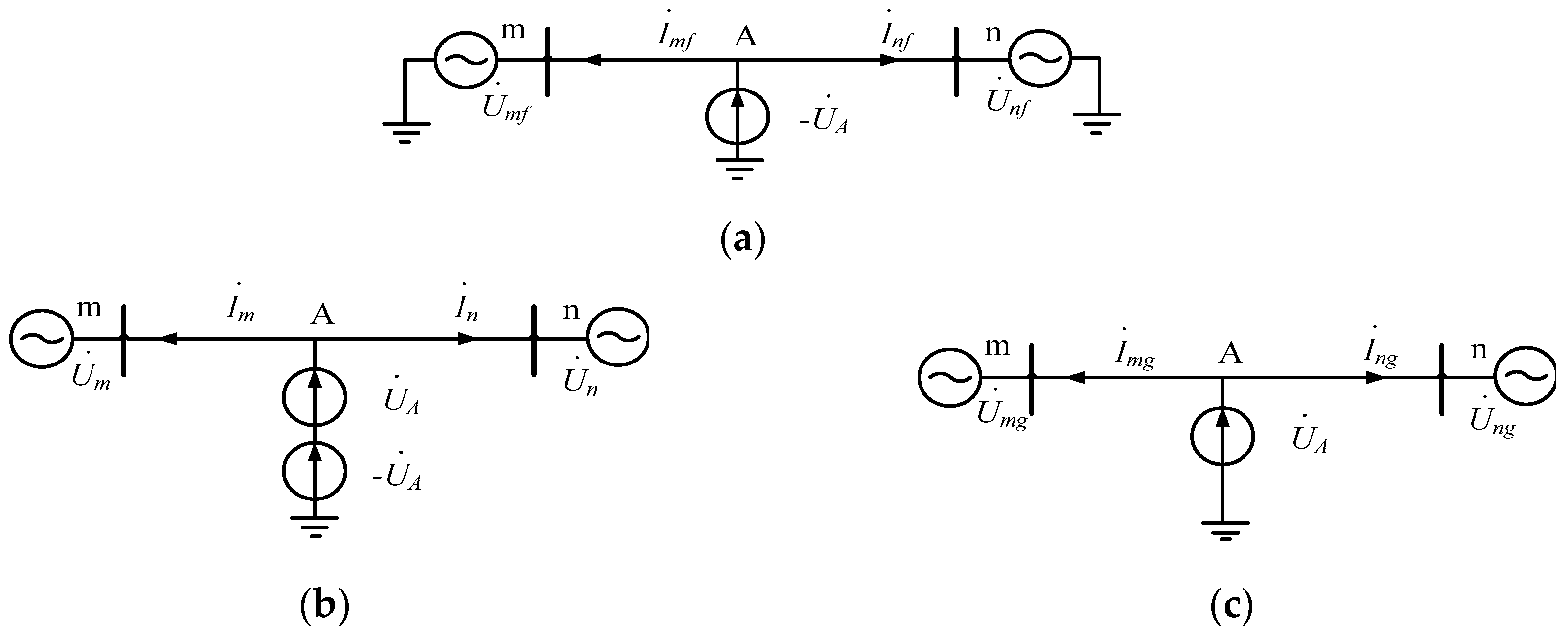
If a short-circuit fault of the three phases occurred, the voltage of each phase would be reduced. If a single-phase fault occurred, the fault phase current would increase, and the currents of the non-fault phases would decrease. The same class of faults has the same features, and different classes of faults have different features [
25,
26]. The power cable fault state (PCFS) can be denoted by the sum of the normal state (NS) and the fault component state (FCS), as indicated in Equation (1) and
Figure 1.
The fault components exist in the added abnormal state of the power cable. The voltage of the fault components can be obtained by the differences between the cable voltage after fault occurrence and the voltage of the normal state. Similarly, the current of the fault components can be obtained by the differences between the cable current after fault occurrence and the current of the normal state.
In a practical system of an online power cable, the
n periods of voltage or current before fault occurrence are regarded as the voltage or current of the normal state. The voltage or current of the fault components
Sg(
t) can be calculated as follows [
27].
where
S(
t) is the voltage or the current after fault occurrence,
T is the power frequency period, and
n is a positive natural number (usually,
n = 2).
The fault component is the voltage difference or current difference of a period. The fault component should also satisfy the time requirement for fault recognition.
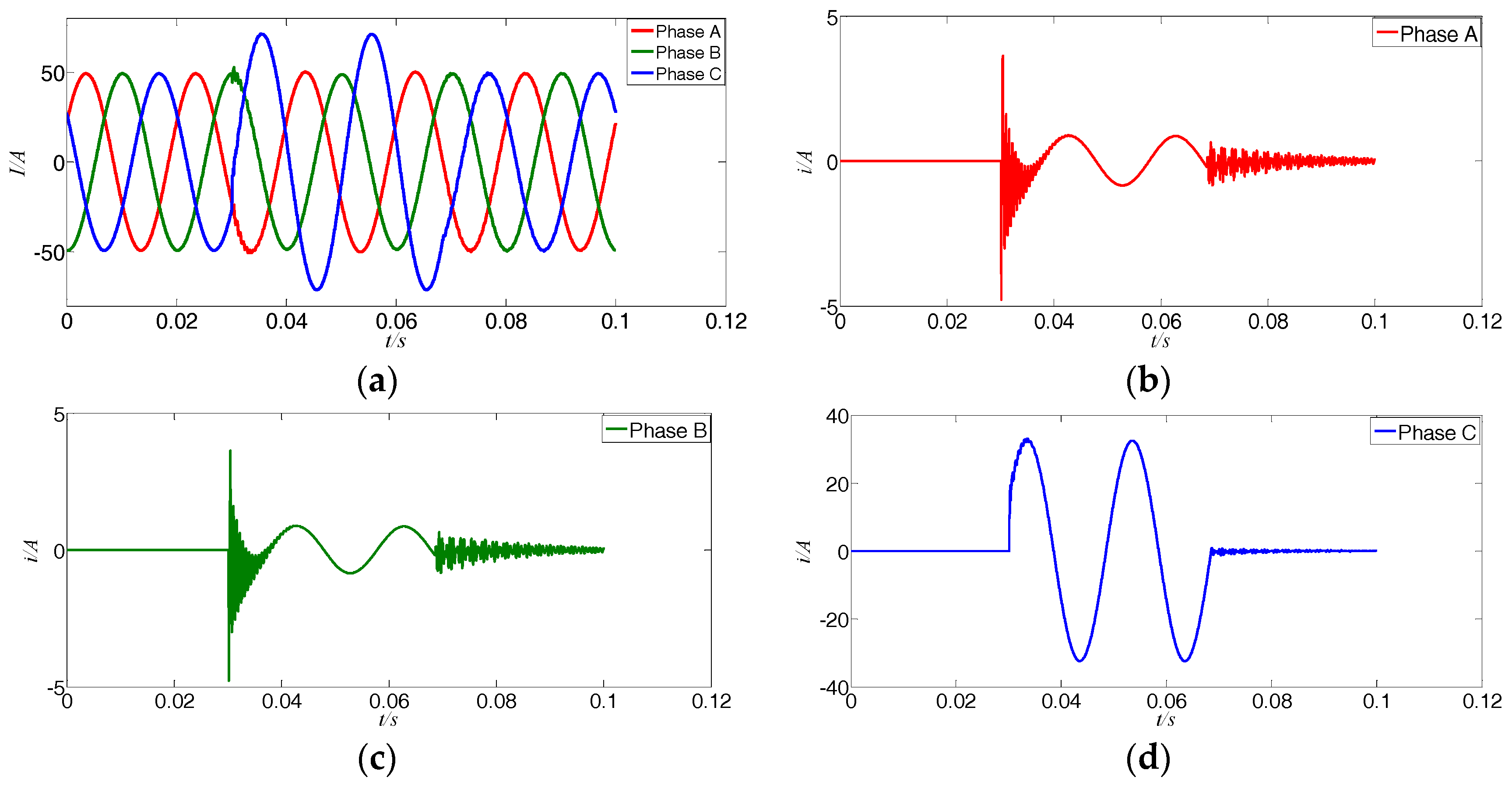
The fault component of the current was taken as the initial signals of the power cable fault in this paper. We used Equation (1) to obtain the fault components of the power cable in the 10 types of short-circuit states. It includes three types of single-phase faults, three types of two-phase faults, three types of two-phase grounded faults, and one type of three-phase faults. The three phase currents and their fault components of the single-phase
A earth faults are shown in
Figure 2. The blue curves are for phase
A, the red curves are for phase
B, and the green curves are for phase
C.
3. The Improved Fractal Box Dimension (IFBD) Recognition Algorithm
The fractal dimension can effectively measure the change of the fine distributed signals, and it keeps invariant if the signals are processed at different scales. Particularly, the box dimension is more suitable for use in calculating a figure or a discrete sport set. Therefore, the box dimension was chosen in this paper as the base to extract the fault feature [
28,
29,
30].
3.1. Definition of the Improved Fractal Box Dimension
The traditional box dimension
Dim (
Sr) of the point set
Sr in a linear space
Rn is
where
n is the length of a side of a square box which covers the point set
Sr.
Nn(
S) represents the minimum number of boxes containing
Sr.
By using the above approximation method, the box dimensions of the fault components of phase
A, phase
B, and phase
C are calculated in the condition of the phase
A earth fault shown in
Figure 1.
Dim (
SA) = 1.56030,
Dim (
SB) = 1.57527,
Dim (
SC) = 1.54622.
For the curves in a plane, their box dimensions always range from one to two. To make the fault classification easier, we can enlarge the distances between the different classes of the 10 types of the short circuit faults. Based on experiments, we defined the improved box dimension
F as follows.
where “tan” represents the tangent function, and
E(
Dim*) is the expectation of the traditional box dimension
Dim of the phase current in the normal state, and it can be written as follows.
where
Sr is the current signals of the power cable in normal state,
, and
m is a positive integer greater than three.
According to Equation (4), we have the improved box dimensions
FA,
FB, and
FC of the fault components of the three phase currents.
where
Dim(
SA),
Dim(
SB), and
Dim(
SC) are the traditional box dimensions of the currents of phase
A,
B, and
C, respectively.
E(
Dim*) is the expectation of the traditional box dimension
Dim of the phase current in the normal state. “tan” represents the tangent function.
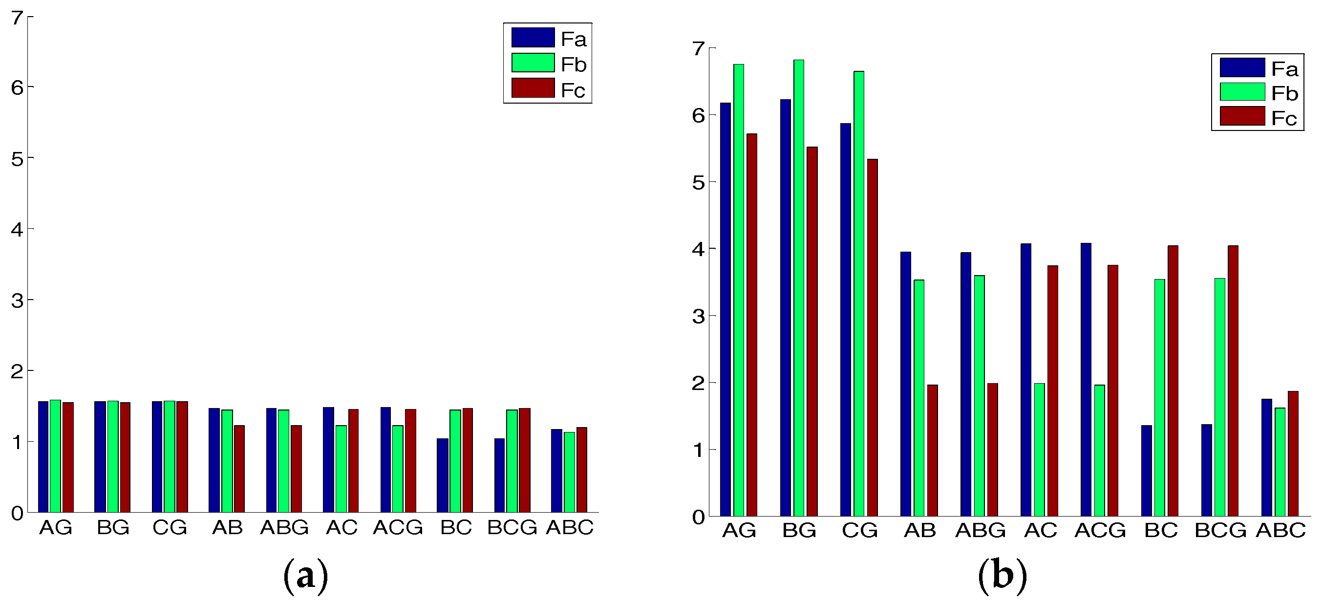
For the 10 detailed classes of the short circuit faults, the fault features using the traditional box dimension and the improved box dimension are shown in
Figure 3a and
Figure 3b respectively. The horizontal axis represents the short circuit faults which include the 10 classes of short circuit faults.
AG,
BG, and
CG are the single-phase short circuit faults.
AB,
BC, and
AC are the phase-between short circuit faults.
ABG,
BCG, and
ACG are the double-phase short circuit faults.
ABC is the three-phase short circuit fault. The vertical axis is the fault feature values. The blue color represents phase
A, the green color represents phase
B, and the red color represents phase
C.
From
Figure 3, it is clear that the traditional box dimension features of the 10 classes are relatively crowded. Compared to the traditional box dimension features, the improved box dimension features of the 10 classes have larger distances among the single-phase fault and the double-phase fault, as well as the three-phase fault. Furthermore, the improved box dimension features have larger distances among the different single-phase faults of
A,
B, and
C. Obviously, the improved box dimension feature is better for short circuit fault recognition of the online power cable than the traditional box dimension feature.
3.2. The Improved Fractal Box Dimension (IFBD) Recognition Algorithm
According to the improved box dimension of Equations (6)–(8), we calculated the improved box dimension features of the short circuits. Based on the calculation results, we found the relationship between the fault classes and the IFBD features, shown in
Table 2 below. We found that the improved box dimension features have a similar relationship in the cases of the two-phase grounded faults and the two-phase-between faults. After the three phase currents or voltages were collected, we could use the relationship to classify the fault.
The three phase currents were chosen as the original signals of the online power cable. The IFBD recognition algorithm could be described as follows.
- Step 1:
Input the three phase currents.
- Step 2:
Extract the current signals of any phase in fault state, and calculate the traditional box dimensions Dim(SA), Dim(SB), and Dim(SC) of the fault components of phase A, B, and C using Equation (3).
- Step 3:
Substitute the traditional box dimensions Dim(SA), Dim(SB), and Dim(SC) respectively into Equations (6)–(8) to calculate the improved box dimension features FA, FB, and FC of the fault components of the three phase currents.
- Step 4:
Classify the short circuit fault according to
Table 2.
4. The Developed Maximum Wavelet Coefficient (DMWC) Recognition Algorithm
In this section, we develop the DMWC recognition algorithm for the single-phase grounded faults (DMWCSP) and the two-phase grounded faults (DMWCTP). Similar to the previous IFBD recognition algorithm, the three phase currents were chosen as the original signals of the online power cable for the DMWC recognition algorithm.
In the fault state, the three phase components are asymmetric and interlocked, so the calculation and analyses are complex. After the K-transform below, we obtained the
α modulus, the
β modulus, and the 0 modulus of the three phases.
where
iA,
iB, and
iC are the three phase currents of the online power cable.
The modulus components of 0,
β, and
α for the different faults are shown in
Table 3. It can be seen that the different classes of faults correspond to different patterns of the modulus
α, modulus
β, and the modulus 0. The DMWC algorithm of DMWCSP and DMWCTP are developed below.
Based on the experiments, the wavelet Db3 were used to analyze the modulus components of
α,
β, and 0 for the different faults. The maximum wavelet coefficients
I0,
Iα, and
Iβ are listed in
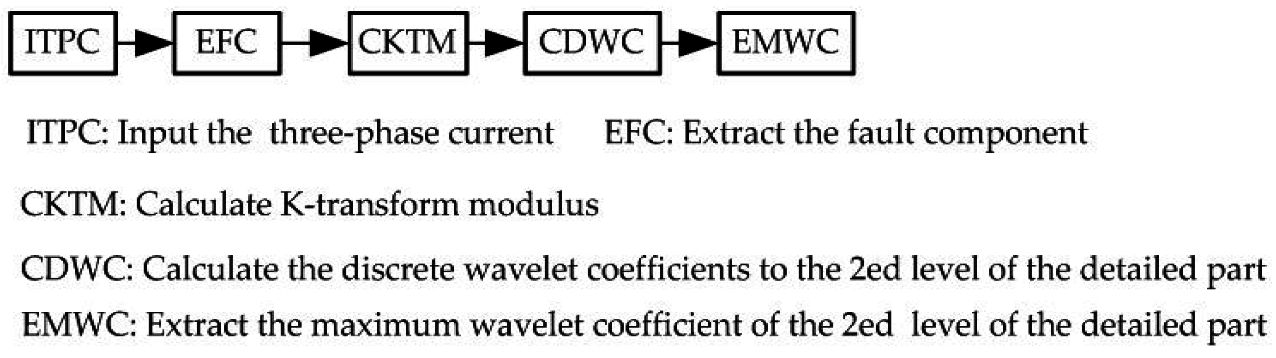
Table 4 for the 10 types of short circuit faults. The flow chart of the calculation of the maximum wavelet coefficients [
31] is shown in
Figure 4.
The proposed DMWCSP algorithm is described below.
- Step 1:
Calculate the modulus components i0, iα, and iβ of the three phase currents iA, iB, and iC by using the K-transform.
- Step 2:
Calculate the maximum wavelet coefficients Iα and Iβ of the modulus components iα and iβ by using the Wavelet transform.
- Step 3:
If Iα < 0.01, then the fault is classified as the grounded fault of C. Otherwise, go to the next step.
- Step 4:
If Iβ < 0.01, then the fault is classified as the grounded fault of B. Otherwise, go to the next step.
- Step 5:
The fault is classified as the grounded fault of A.
Similar to the proposed DMWCSP algorithm, the proposed DMWCTP algorithm was described below to support DMWC recognition algorithm.
- Step 1:
Calculate the modulus components i0, iα, and iβ of the three phase currents iA, iB, and iC by using the K-transform.
- Step 2:
Calculate the maximum wavelet coefficients I0 of the modulus components i0 by using the Wavelet transform.
- Step 3:
If I0 < 0.01, then the fault is classified as the two-phase grounded fault of AB, AC, or BC. Otherwise, the fault is classified as the two-phase-between fault of AB, AC, or BC.
5. The Proposed Fusion Sensing Method
From the above studies, it was found that the IFBD recognition algorithm could recognize the single-phase fault, double-phase faults, and the three-phase fault easily. Additionally, it had a slight advantage in classifying the detailed single-phase faults of A, B, and C. In contrast, the DMWCSP and DMWCTP algorithms could recognize the detailed single-phase faults of A, B, and C. However, they had relative difficultly in recognizing the detailed double-phase faults of AB, AC, and BC.
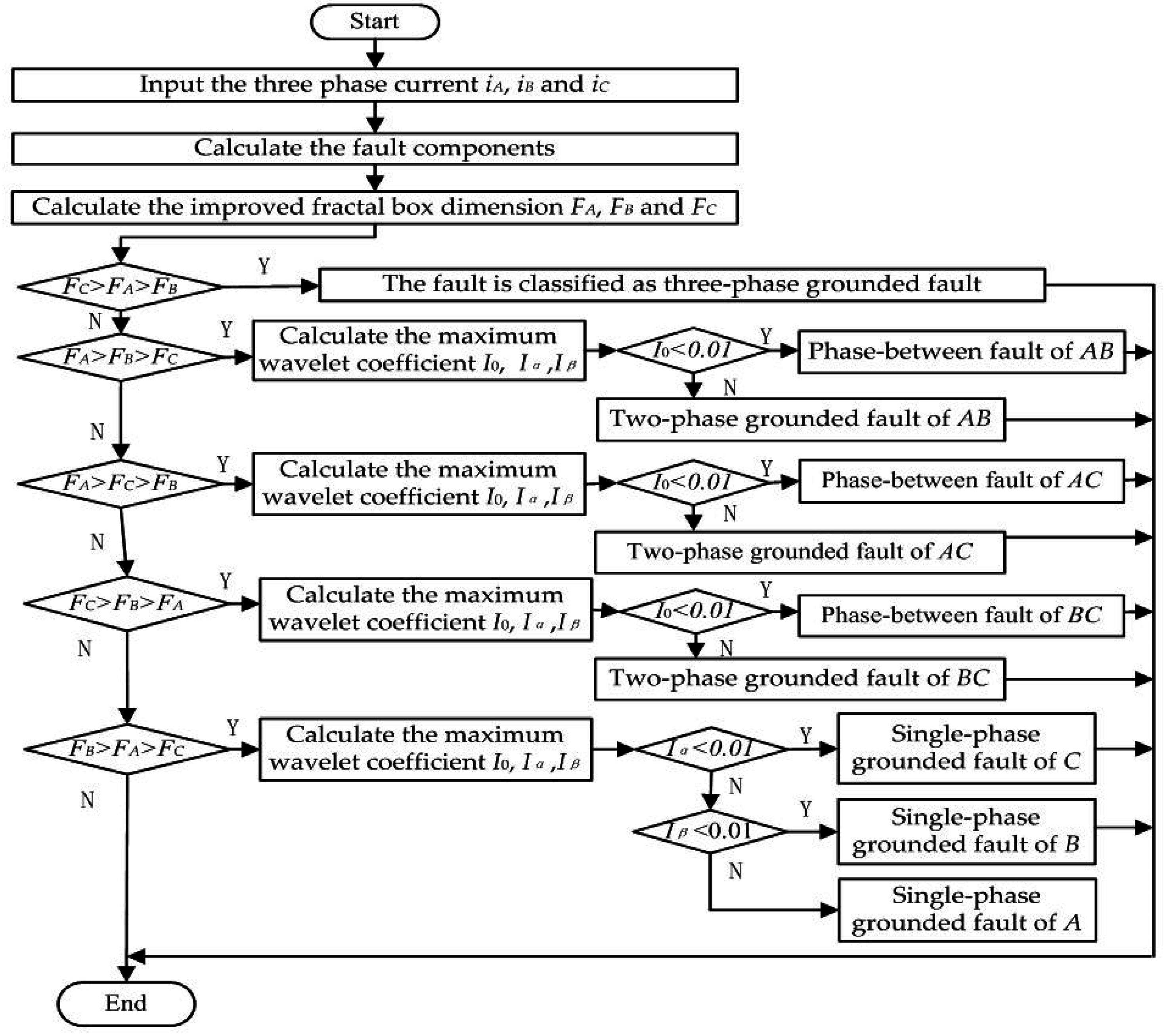
The flow chart of the FS method is shown in
Figure 5. The FS method is described below.
- Step 1:
Input the real-time three-phase currents IA, IB, and IC.
- Step 2:
Extract the fault components ia, ib, and ic according to Equation (2).
- Step 3:
Calculate the improved box dimension features FA, FB, and FC of the fault components of the three phase currents by using Equations (6)–(8).
- Step 4:
If FC > FA > FB, the fault is classified as the three-phase fault. Otherwise, go to the next step.
- Step 5:
If FA > FB > FC, classify the fault as the phase-between fault of AB if I0 < 0.01 or as the two-phase grounded fault of AB if I0 > 0.01. Otherwise, go to the next step.
- Step 6:
If FA > FC > FB, classify the fault as the phase-between fault of AC if I0 < 0.01 or as the two-phase grounded fault of AC if I0 > 0.01. Otherwise, go to the next step.
- Step 7:
If FC > FB > FA, classify the fault as the phase-between fault of BC if I0 < 0.01 or as the two-phase grounded fault of BC if I0 > 0.01. Otherwise, go to the next step.
- Step 8:
If FB > FA > FC, classify the fault as the single-phase grounded fault of C if Iα < 0.01 or as the single-phase grounded fault of B if Iβ > 0.01. Otherwise, classify the fault as the single-phase grounded fault of A.
6. Experiment and Results
6.1. Experimental Environment
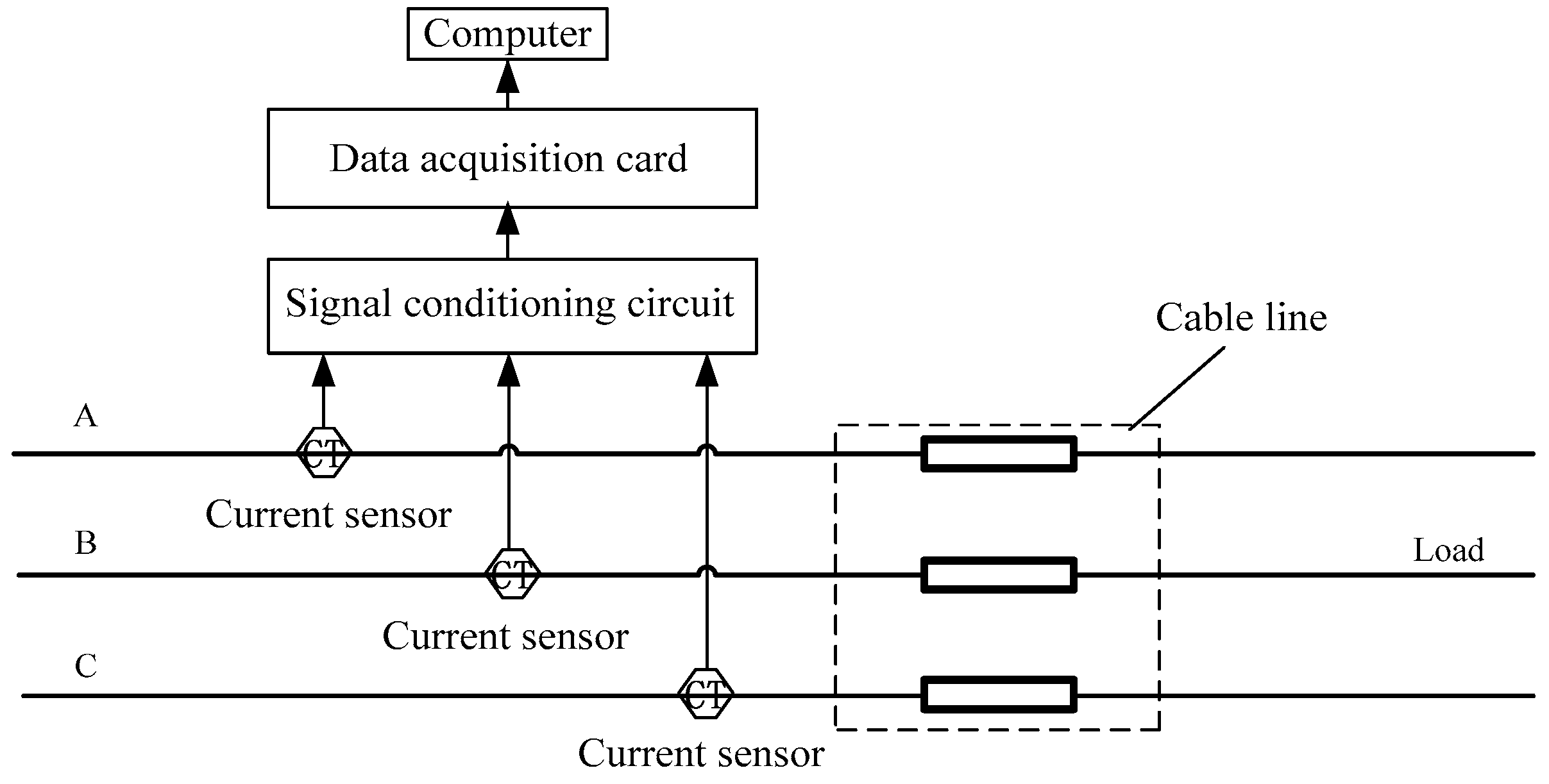
The experimental system structure is shown in
Figure 6.
The LabVIEW software was used for the interface platform. The diameter of the power cable was 2.5 mm. The power supply was the three phase variable-frequency power SPS-HL-3300 N, which changed the voltage from 380 V to 90 V.
The star connection mode was used with the neutrals grounded. The signal collection card was a NI PCI-9203. The closed-loop Hoare current sensors CHB-25NP were from Beijing SENSOR Electronics Co., Ltd. (Beijing, China).
6.2. Experiment Results and Analysis
Table 5 shows the IFBD recognition process and the results with an initial angle of 30° and a fault resistance of 30 Ω.
Table 6 shows the DMWC recognition process and the results with the initial angle of 30° and fault resistances of 30 Ω and 300 Ω.
Table 7 shows the comparison of the DMWC recognition method and the FS method with different initial angles 0°, 30°, and 90°, and fault resistances of 30 Ω, 150 Ω, and 300 Ω.
Table 8 shows the comparison of the DMWC recognition method and the FS method with different initial angles of 0° and 30°, and different fault distances of 0.8 km, 8 km, and 30 km.
It can be seen from
Table 5 that the IFBD recognition algorithm could classify 8 of the 10 types of short circuit faults. It could recognize the single-phase grounded faults, but could distinguish the detailed fault phase of
A,
B, or
C.
The experiments proved that the DMWC recognition algorithm could correctly classify all 10 types of short circuit faults. In addition, the fault resistances had no influence on the recognition result of the DMWC recognition algorithm. Therefore, this algorithm is better than the IFBD recognition algorithm regarding fault type recognition.
It can be seen from
Table 7 and
Table 8 that the FS method could correctly classify all 10 types of short circuit faults. The initial angle, the fault resistance, and the fault distance had no influence on the recognition result of the FS method. Therefore, the FS method is better than the IFBD recognition algorithm and the DMWC recognition algorithm regarding their comprehensive performances.
7. Conclusions
The IFBD algorithm was developed to enlarge the distances between 10 classes of short circuit faults by using the improved fractal dimension feature extracted from the three-phase currents for the first stage of fault recognition. K-transform and wavelet analysis were then used to establish the relationship between the modulus value and the fault class, and the DMWC recognition algorithm was developed. The IFBD algorithm and the DMWC algorithm were then combined to produce the FS method. Finally, the test system was utilized with the LabVIEW platform. The FS method was experimentally proven to effectively recognize all 10 classes of short circuit faults. The FS method was also not influenced by the parameters of the initial angle, transient resistance, and the fault distance. Compared with the DMWC algorithm, the FS method improved the recognition accuracy from 80.3% to 96.3% in the case of varied fault resistances, and improved the recognition accuracy from 87.8% to 98.0% in the case of varied fault distances.
Acknowledgments
This research was sponsored by the Natural Science Foundation of China (51405381), the Key Scientific and Technological Project of Shaanxi Province (2016GY-040), and the Science Foundation of Xi’an University of Science and Technology (104-6319900001).
Author Contributions
M.W. conceived and designed the experiments; L.Z. and Y.G. performed the experiments; M.W. and L.Z. and Y.G. analyzed the data; M.W. and L.Z. and Y.G. wrote the paper.
Conflicts of Interest
The authors declare no conflict of interest.
References
- Zhao, J.H.; Xu, Y.; Luo, F.J.; Dong, Z.Y.; Peng, Y.Y. Power system fault diagnosis based on history driven differential evolution and stochastic time domain simulation. Inf. Sci. 2014, 275, 13–14. [Google Scholar] [CrossRef]
- Prasad, A.; Edward, J.B. Application of Wavelet Technique for Fault Classification in Transmission. Procedia Comput. Sci. 2016, 92, 78–81. [Google Scholar] [CrossRef]
- Jun, J.T.; Feng, P.F.; Wei, S.L.; Zhang, H.; Liu, Y.F. Investigation on the surface morphology of Si3N4 ceramics by a new fractal dimension calculation method. Appl. Surf. Sci. 2016, 387, 813–817. [Google Scholar]
- Guclu, S.O.; Ozcelebi, T.; Lukkien, J. Distributed Fault Detection in Smart Spaces Based on Trust Management. Procedia Comput. Sci. 2016, 83, 66–70. [Google Scholar] [CrossRef]
- Bharata, M.J.; Gopakumar, P.; Mohanta, D.K. A novel transmission line protection using DOST and SVM. Eng. Sci. Technol. 2016, 19, 1027–1037. [Google Scholar]
- Lin, S.; Mei, J.T.; Chen, S.; He, Z.Y.; Qian, Q.Q. Fault Detection and Faulty Phase Determination of Transmission Lines Based on Time-Frequency Characteristics of Transient Travelling Waves. Power Syst. Technol. 2012, 36, 49–52. [Google Scholar]
- Chicharro, F.I.; Cordero, A.; Torregrosa, J.R. Dynamics and Fractal Dimension of Steffensen-Type Methods. Algorithms 2015, 8, 271–279. [Google Scholar] [CrossRef]
- Gómez, M.J.; Castejón, C.; García-Prada, J.C. Review of Recent Advances in the Application of the Wavelet Transform to Diagnose Cracked Rotors. Algorithms 2016, 9, 19. [Google Scholar] [CrossRef]
- Zhou, W.; Xiong, J.; Li, F.; Jiang, N.; Zhao, N. Fusion of Multiple Pyroelectric Characteristics for Human Body Identification. Algorithms 2014, 7, 685–702. [Google Scholar] [CrossRef]
- Tan, X.H.; Liu, J.Y.; Li, X.P.; Zhang, L.H.; Cai, J.C. A simulation method for permeability of porous media based on multiple fractal model. Int. J. Eng. Sci. 2015, 95, 76–80. [Google Scholar] [CrossRef]
- Yu, M.Z.; Chan, T.L. A bimodal moment method model for submicron fractal-like agglomerates undergoing Brownian coagulation. J. Aerosol Sci. 2015, 88, 25–30. [Google Scholar] [CrossRef]
- Martino, G.D.; Iodice, A.; Riccio, D.; Ruello, G.; Zinno, I. Angle Independence Properties of Fractal Dimension Maps Estimated From SAR Data. IEEE J. Sel. Top. Appl. Earth Obs. Remote Sens. 2013, 6, 1242–1248. [Google Scholar] [CrossRef]
- Nelson, J.D.B.; Kingsbury, N.G. Fractal dimension, wavelet shrinkage and anomaly detection for mine hunting. IET Signal Process. 2012, 6, 485–487. [Google Scholar] [CrossRef]
- Reza, F.M.; Qi, X.J. Face Recognition under Varying Illumination with Logarithmic Fractal Analysis. IEEE Signal Process. Lett. 2014, 21, 1459–1460. [Google Scholar]
- Xu, Y.; Liu, D.L.; Quan, Y.H.; Callet, P.L. Fractal Analysis for Reduced Reference Image Quality Assessment. IEEE Trans. Image Process. 2015, 24, 2099–2100. [Google Scholar] [CrossRef] [PubMed]
- Tumu, I.; Concas, G.; Marchesi, M.; Tonelli, R. The fractal dimension of software networks as a global quality metric. Inf. Sci. 2013, 245, 295–299. [Google Scholar]
- Liu, J.H.; Liang, R.; Wang, C.L.; Fan, D.P. Application of fractal theory in detecting low current faults of power distribution system in coal mines. Min Sci. Technol. (China) 2009, 19, 321–323. [Google Scholar] [CrossRef]
- Usama, Y.; Liu, X.M.; Imam, H.; Sen, C.; Kar, N.C. Design and implementation of a wavelet analysis-based shunt fault detection and identification module for transmission lines application. IET Gener. Transm. Distrib. 2014, 8, 431–440. [Google Scholar] [CrossRef]
- Zhang, S.W.; Zhang, F.; Wang, Z.J.; Gu, H.Y.; Ning, Q. Series Arc Fault Identification Method Based on Energy Produced by Wavelet Transformation and Neural Network. Trans. China Electrotech. Soc. 2014, 29, 291–293. [Google Scholar]
- Gopakumar, P.; Reddy, M.J.B.; Mohanta, D.K. Transmission line fault detection and localisation methodology using PMU measurements. IET Gener. Transm. Distrib. 2015, 9, 1033–1039. [Google Scholar] [CrossRef]
- Zhang, L.L.; Xu, B.Y.; Xue, Y.D.; Gao, H.L. Transient Fault Locating Method Based on Line Voltage and Zero-mode Current in Non-solidly Earthed Network. Proc. CSEE 2012, 32, 110–113. [Google Scholar]
- Prasad, A.; Edward, J.B. Application of Wavelet Technique for Fault Classification in Transmission Systems. Procedia Comput. Sci. 2016, 92, 78–83. [Google Scholar] [CrossRef]
- Dai, H.Z.; Zheng, Z.B.; Wang, W. A new fractional wavelet transform. Commun. Nonlinear Sci. Numer. Simul. 2017, 44, 19–32. [Google Scholar] [CrossRef]
- Wu, Q.; Law, R. Complex system fault diagnosis based on a fuzzy robust wavelet support vector classifier and an adaptive Gaussian particle swarm optimization. Inf. Sci. 2010, 180, 4515–4520. [Google Scholar] [CrossRef]
- Zheng, G.P.; Zhang, L.; Jiang, C.; Qi, Z.; Yang, Y.H. Line and Segment Online Location of Single-phase-to-earth Fault in the Ungrounded Neutral System. Autom. Electr. Power Syst. 2013, 37, 111–113. [Google Scholar]
- Jiang, J.A.; Chuang, C.L.; Wang, Y.C.; Hung, C.H.; Wang, J.Y.; Lee, C.H.; Hsiao, Y.T. A Hybrid Framework for Fault Detection, Classification, and Location—Part I: Concept, Structure, and Methodology. IEEE Trans. Power Deliv. 2011, 26, 1990–1998. [Google Scholar] [CrossRef]
- Tang, G.; Hou, W.; Wang, H.Q.; Luo, G.G.; Ma, J.W. Compressive Sensing of Roller Bearing Faults via Harmonic Detection from Under-Sampled Vibration Signals. Sensors 2015, 15, 25648–25660. [Google Scholar] [CrossRef] [PubMed]
- Wook, K.J.; Kim, J.H.; Seo, J. Multiple Leader Candidate and Competitive Position Allocation for Robust Formation against Member Robot Faults. Sensors 2015, 15, 10777–10780. [Google Scholar]
- Han, C.; Zhang, H.Y.; Guo, C.X.; Jiang, C.; Sang, N.; Zhang, L.P. A Remote Sensing Fusion Method Based on the Analysis Sparse Model. IEEE J. Sel. Top. Appl. Earth Obs. Remote Sens. 2016, 9, 1302–1308. [Google Scholar] [CrossRef]
- Xu, J.D.; Yu, X.C.; Pei, W.J.; Hu, D.; Zhang, L.B. A remote sensing fusion method based on feedback sparse component analysis. Comput. Geosci. 2015, 85, 116–118. [Google Scholar] [CrossRef]
- Cheng, J.; Liu, H.J.; Liu, T.; Wang, F.; Li, H.S. Remote sensing image fusion via wavelet transform and sparse representation. ISPRS J. Photogramm. Remote Sens. 2015, 104, 160–170. [Google Scholar] [CrossRef]
© 2016 by the authors; licensee MDPI, Basel, Switzerland. This article is an open access article distributed under the terms and conditions of the Creative Commons Attribution (CC-BY) license (http://creativecommons.org/licenses/by/4.0/).


