Review

An Overview on the Applications of Matrix Theory in Wireless Communications and Signal Processing

Department of Electrical and Computer Engineering, Texas A&M University, College Station, TX 77843, USA
*
Author to whom correspondence should be addressed.
Algorithms 2016, 9(4), 68; https://doi.org/10.3390/a9040068
Submission received: 26 June 2016 / Revised: 8 September 2016 / Accepted: 5 October 2016 / Published: 14 October 2016

Abstract

:
This paper overviews the key applications enabled by matrix theory in two major fields of interest in electrical engineering, namely wireless communications and signal processing. The paper focuses on the fundamental role played by matrices in modeling and optimization of wireless communication systems, and in detection, extraction and processing of the information embedded in signals. Among the major applications in wireless communications, the role of matrix representations and decompositions in characterizing multiple-input multiple-output (MIMO) and orthogonal frequency division multiplexing (OFDM) communication systems is described. In addition, this paper points out the important contribution made by matrices in solving signal estimation and detection problems. Special attention is given to the implementation of matrices in sensor array signal processing and the design of adaptive filters. Furthermore, the crucial role played by matrices in representing and processing digital images is depicted by several illustrative applications. This paper concludes with some applications of matrix theory in the area of compressive sensing of signals and by outlining a few open research problems for future study.

1. Introduction

Matrix theory is widely used in many disciplines of modern engineering, including wireless communications, signal processing, control, biomedical engineering, etc. From a mathematical perspective, matrices are used both as a representation as well as an information processing tool to solve efficiently and reliably practical engineering problems. Since matrices are prevalent in engineering and have enabled remarkable solutions to problems of paramount importance, this paper overviews some of the major applications of matrix theory in wireless communications and signal processing. Our hope is that this article will help in renewing the interest of engineering community in linear algebra, and in particular in the tools offered by matrix theory, and its applications in engineering. Rather than describing details for all the statements and developments, our goal is instead to provide the readers the basic facts and key features of how matrix techniques were applied in some major engineering applications that played a fundamental role during the last two decades in the fields of signal processing and wireless communications.
The outline of this paper is summarized as follows. Section 2 describes how matrix techniques are exploited in the modern communication systems. Specifically, we discuss the key role played by the concept of singular value decomposition (SVD) in modeling and characterization of the multiple-input multiple-output (MIMO) or multiple antennas based communication systems, and the important role played by unitary matrix transformations such as Discrete Fourier Transform (DFT) in the orthogonal frequency-division multiplexing (OFDM) signaling scheme, which currently has been adopted in many wireless communications standards. Section 3 focuses on several illustrative uses of matrices in signal estimation and detection applications. In particular, the usefulness of matrix decompositions and matrix inversion lemma in enabling online (recursive) estimation of parameters and development of adaptive filters is illustrated. A special attention is also given to the applications of matrices in sensor array signal processing. A more modern estimation method based on large dimensional random matrix theory is also briefly discussed to exemplify the recent trends in the utilization of matrices in signal processing and wireless communications. Section 4 describes the close relationship between matrices and images. Two image compression methods, which rely on matrix transformation and separation operations, are described. In Section 5, a recently proposed data compression approach termed as compressive (compressed) sensing is briefly examined from the perspective of the role played by matrices. Finally, Section 6 concludes the paper by outlining the key role played by matrices in solving some important problems from the fields of signal processing and wireless communications. Several open research problems that require more advanced linear algebra concepts and results are pointed out as well.
Throughout this paper, we will denote scalars by lowercase italic letters (a), vectors by bold lowercase italic letters ( a ), and matrices by bold uppercase Roman letters ( A ).

2. Matrix Theory in Modern Wireless Communication Systems

Nowadays, wireless communications have emerged as the fastest growing segment of the telecommunications industry. For example, cellular communication systems have exhibited an explosive growth over the last several decades and currently present over 6 billion users all over the world. Existing and future applications of wireless communications include multimedia Internet-based cell phones, high-quality real-time streaming of video and data signals, and transmission, reception and processing of all sorts of data collected by sensors and devices. The requirements imposed by these communication systems are subject to many technical challenges. In this section, two modern signaling schemes: MIMO and OFDM, which are currently adopted in many wireless communications standards to improve the performance of current wireless communication systems, are discussed. The presentation will focus mainly on how the matrix theory concepts and results can be applied to implement and assess the performance of MIMO and OFDM-based communications systems.

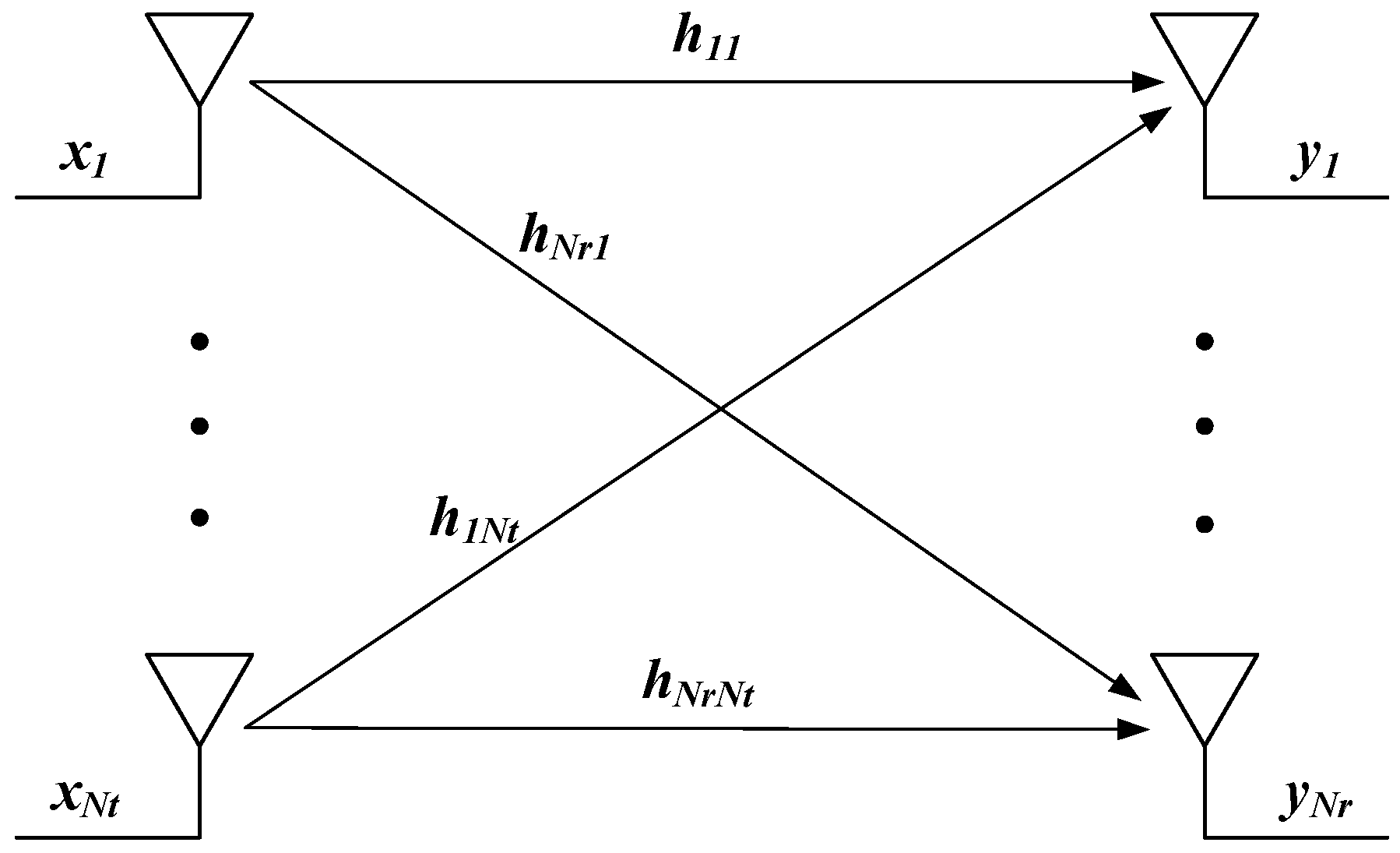
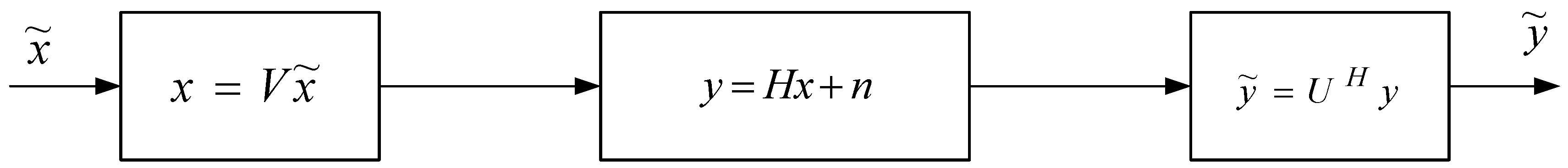
2.1. SVD for Modeling MIMO Channels

The channel capacity, defined as the maximum data rate at which data can be sent with arbitrarily low probability of error, was reported for the Gaussian channel by Shannon in his seminal paper [1]. Currently, achieving higher and higher data rates with tolerable error rates and fixed transmitter power is one of the most demanding targets for the current wireless communication systems. For example, the evolution from LTE to 4 G LTE-Advanced communication standard requires an increase in the downlink data rate from 150 Mbps to 1 Gbps and an uplink data rate increase from 75 Mbps to 500 Mps [2].
Theoretically, there are many ways to improve the channel capacity, like increasing the signal power, reducing the noise power, exploitation of space/time/frequency diversity, multiplexing, etc. However, due to the power limitation and unexpected properties of the receiver noise, diversity and multiplexing have been two popular design strategies on which researchers focused extensively during the last decade. Among these techniques, using multiple transmit and multiple receive antennas has been advocated as one of the most efficient methods to achieve the spatial multiplexing gain.
MIMO signaling is defined as the communication system with multiple antennas at both the transmitter and receiver, and it can be modeled as a system with multiple inputs and multiple outputs. A MIMO communication system with N t transmit and N r receive antennas is shown in Figure 1. This system can be depicted by the following matrix representation:
y 1 y N r = h 11 h 1 N t h N r 1 h N r N t x 1 x N t + ν 1 ν N r ,
or simply by y = H x + ν , where x represents the N t × 1 dimensional vector of transmitted data symbols, y denotes the N r × 1 dimensional vector of received data symbols, H = [ h i j ] stands for the transmit (propagation channel) matrix with the entry h i j denoting the gain from transmitter j to receiver i, and ν is assumed to represent the white Gaussian noise vector. From (1), one can infer that
y i = j = 1 N t h i j x j + ν i , i = 1 , 2 , , N r .
In other words, the output symbol y i is a linear combination of the input symbols, which makes it difficult to recover the transmitted data symbols. This unfavorable phenomenon is referred to as the intersymbol interference (ISI) and results in signal aliasing. However, it is shown next that the MIMO channel can be decomposed into independent signal paths by the help of SVD. This feature enables to design efficient decoding schemes while achieving the spatial multiplexing gain to improve the channel capacity. The SVD representation of channel matrix H takes the form:
H = U Σ V H ,
where U C N r × N r and V C N t × N t are unitary matrices, Σ R N r × N t is a diagonal matrix with r nonzero diagonal elements, where r min ( N r , N t ) . The parallel decomposition of the MIMO channel into a series of parallel single-input single-output (SISO) channels can be obtained by pre-multiplying the transmitted signal with V and post-multiplying the received signal with U H , as shown in Figure 2.
In the new coordinate system, the relationship between the input and output of channel takes the form:
y ˜ = U H ( H x + ν ) = U H ( H V x ˜ + ν ) = U H ( U Σ V H V x ˜ + ν ) = Σ x ˜ + ν ˜ .
Assume Σ = diag ( σ 1 , σ 2 , , σ r , 0 , , 0 ) . Thus, the MIMO channel can be decomposed into r independent SISO channels. Specifically, the ith SISO channel has a gain σ i and a noise factor ν ˜ i , and assumes the representation
y ˜ i = σ i x ˜ i + ν ˜ i .
This implies that all the efficient signaling and decoding strategies well investigated in the SISO context could be transferred mutatis-mutandis to the MIMO framework with a minimal effort thanks to SVD.
Moreover, by assuming that the channel state information, or equivalently, the channel matrix H is known at the receiver but not at the transmitter, Telatar [3] showed that the MIMO channel capacity can be expressed as
C = i = 1 r log 2 1 + σ i 2 ρ N t ,
where ρ is the transmitted signal power and the additive receiver noise is assumed to have unit power. This result is in perfect accordance with (3) since the MIMO capacity in (4) can be interpreted as the summation of independent SISO channel capacities. Under the assumption that the entries of H follow a zero-mean spatially white (ZMSW) model, the law of large numbers implies that lim N t 1 N t H H H = I N r , and the capacity can be expressed asymptotically [4] in the presence of a large number of transmit/receive antennas as
C = N r log 2 ( 1 + ρ ) .
This implies that as N = min ( N r , N t ) grows large, the channel capacity increases linearly with N [5]. This fact as well as some other results for MIMO capacity analysis [6,7] makes MIMO signaling superior to SISO signaling and it also explains the reason why currently MIMO techniques are so appealing in a broad range of applications such as wireless communications, radar, sonar, geo-physical (seismic) signal processing, wireless sensor networks, and antenna array processing. The proposed framework for determining the capacity of MIMO linear time-invariant channels could be further extended to determine the capacity of memoryless nonlinear MIMO channels subject to a power constraint [8]. Reference [8] re-formulates this problem within a functional framework and employs variational calculus techniques to determine the capacity-achieving input distribution of memoryless nonlinear MIMO channels. As a special case, the capacity-achieving input distribution for the linear MIMO channel is re-established in [8].

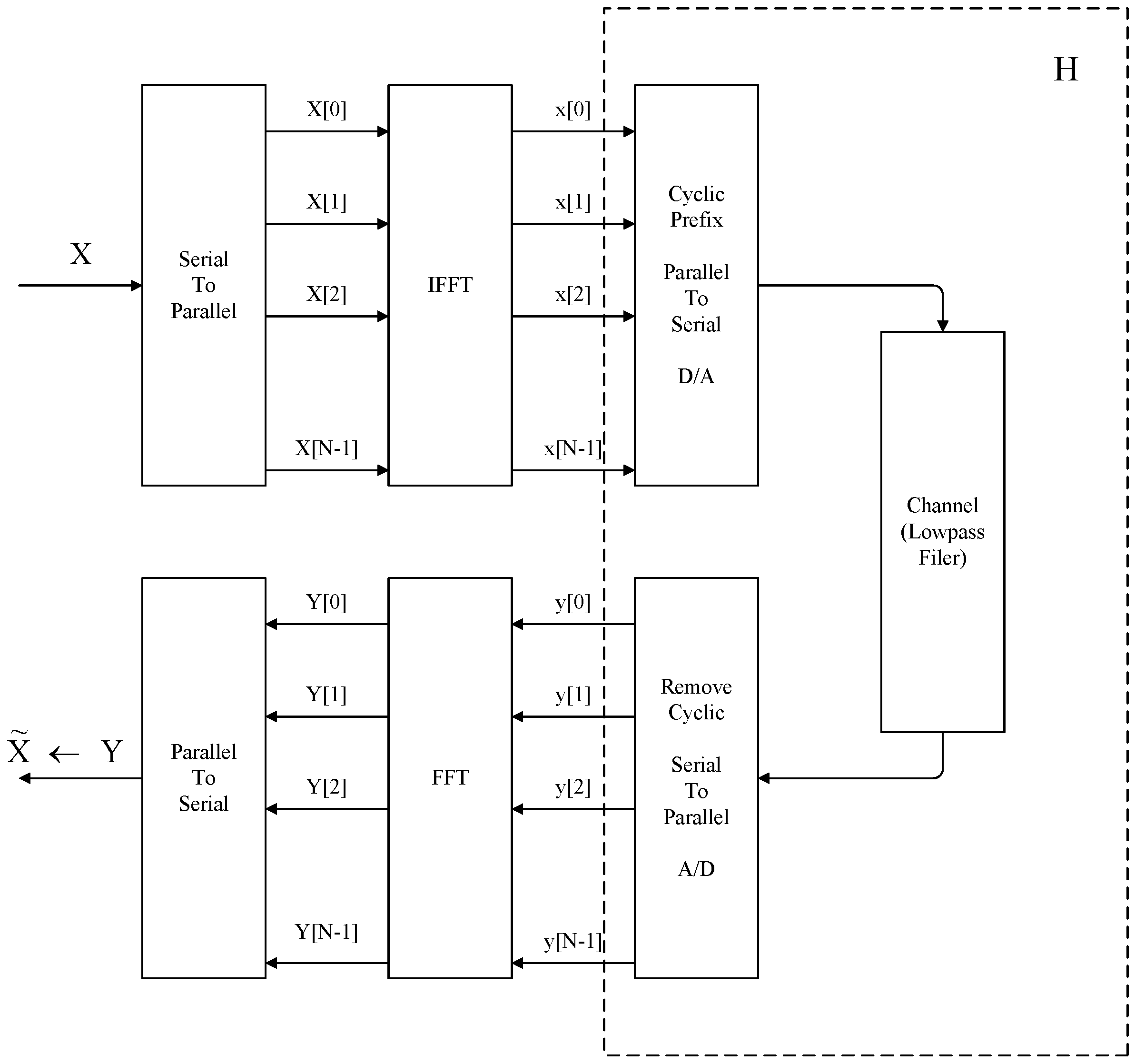
2.2. Matrix Representation of OFDM

Orthogonal frequency-division multiplexing (OFDM) is another core technology employed by modern wireless communication systems. It is the basic signaling technology in the recently proposed long-term evolution (LTE) wireless communication standard and has been already adopted as the basic signaling scheme in many communication standards such as Wireless Local Area Network (WLAN), Wireless Metropolitan Area Network (WMAN), Wireless Regional Area Network (WRAN), Wireless Personal Area Network (WPAN), Digital Audio Broadcasting (DAB), and Digital Video Broadcasting (DVB). OFDM represents a multicarrier system which divides the whole spectrum into several narrow frequency bands, and the data is transmitted in a parallel manner along all these narrow frequency bands. The basic signaling mechanism of OFDM [4] is depicted graphically in Figure 3.
To simplify the exposition, we have represented all the operations between channel input vector x and output vector y as a system with transfer matrix H , such that y = H x + ν , where ν stands for the additive noise vector. OFDM implements an inverse discrete Fourier transform (IDFT) at the transmitter side and a discrete Fourier transform (DFT) at the receiver side. However, in practice, the fast Fourier transform (FFT) algorithm is widely used to compute DFT due to its fast implementation and computational efficiency. This is the reason why the processing blocks are marked in Figure 3 with FFT and IFFT instead of DFT and IDFT.
Given x [ n ] , n = 0 , 1 , , N 1 , the N-point DFT of x [ n ] is defined as
X [ k ] = 1 N n = 0 N 1 x [ n ] e j 2 π n k N , k = 0 , 1 , , N 1 .
The sequence x [ n ] can be recovered back by means of the IDFT as
x [ n ] = 1 N k = 0 N 1 X [ k ] e j 2 π n k N , n = 0 , 1 , , N 1 .
It is easy to show that the DFT operation can be represented as a matrix multiplication
X = W x ,
where X = [ X [ 0 ] , X [ 1 ] , , X [ N 1 ] ] T , x = [ x [ 0 ] , x [ 1 ] , , x [ N 1 ] ] T , and the DFT matrix W is a unitary matrix expressed as
W = 1 N 1 1 1 1 1 w w 2 w N 1 1 w 2 w 4 w 2 ( N 1 ) 1 w N 1 w 2 ( N 1 ) w ( N 1 ) 2
with w = e j 2 π N . Additionally, the IDFT operation can be expressed as
x = W 1 X = W H X ,
since W 1 = W H is due to the fact that W is a unitary matrix.

Matrix Analysis of OFDM

Consider a discrete channel H with coefficients h [ n ] , n = 0 , 1 , , M . The cyclic prefix [4] is implemented to generate the new sequence x ˜ [ n ] , n = M , M + 1 , , N 1 , where x ˜ [ n ] = x [ n mod N ] . Specifically,
x ˜ [ M ] , , x ˜ [ 1 ] , x ˜ [ 0 ] , , x ˜ [ N 1 ] = x [ N M ] , , x [ N 1 ] , x [ 0 ] , , x [ N 1 ] .
This yields the output y [ n ] = x ˜ [ n ] * h [ n ] + ν [ n ] . Introducing the simplified notations x ˜ [ n ] as x ˜ n , h [ n ] as h n , etc., it turns out that the relation between the input and output of the channel can be expressed as
y N 1 y N 2 y 0 = h 0 h 1 h M 0 0 0 h 0 h M 1 h M 0 0 0 0 h 0 h M 1 h M x ˜ N 1 x ˜ 0 x ˜ 1 x ˜ M + ν N 1 ν N 2 ν 0 .
Plugging (6) into (7) leads to
y N 1 y N 2 y 0 = h 0 h 1 h M 0 0 0 h 0 h M 1 h M 0 0 0 h 0 h M 1 h M h 2 h 3 h M 2 h 0 h 1 h 1 h 2 h M 1 0 h 0 x N 1 x N 2 x 0 + ν N 1 ν N 2 ν 0 ,
which can be written compactly as
y = H x + ν .
It turns out that H is a circulant matrix with the generator vector [ h 0 , 0 , , 0 , h M , , h 1 ] T . According to the properties of circulant matrices [9], H admits the eigenvalue decomposition
H = U Λ U H ,
where Λ is a diagonal matrix whose diagonal elements stand for the eigenvalues of H and U is a unitary matrix whose rows correspond to the columns of DFT matrix W in (5). In other words, U = W H . Thus, one can infer the following relations:
Y = W y = W ( H x + ν ) = W ( H W H X + ν ) = W U Λ U H W H X + W ν = Λ X + ν ˜ .
It turns out that by exploiting DFT and IDFT operations and inserting the cyclic prefix, OFDM transforms a frequency-selective channel into N orthogonal flat-fading subchannels without ISI, which helps to reduce the complexity of the receiver decoder. Due to its advantages in combining the energy of all the propagation paths of the channel and enabling a reduced complexity equalization, OFDM has been adopted in numerous communications standards (ADSL, WLAN, LTE, etc.) and has been also used in conjunction with the MIMO technique in what it is currently referred to as the MIMO-OFDM technology [10].

3. Matrix Applications in Signal Estimation Theory

Estimation theory is a branch of statistics that aims to estimating the values of parameters based on measured or empirical data. Applications of parameter estimation are prevalent in the area of wireless communications and signal processing. In this section, we briefly discuss how matrix theory can be applied to simplify signal estimation problems, reduce computational complexity, develop adaptive (recursive) filters and solve ill-conditioned estimation problems.

3.1. Cholesky Decomposition for Whitening the Noise

The Cholesky decomposition [11] of a Hermitian positive-semidefinite matrix A admits the representation:
A = D D H ,
where D is a lower triangular matrix with nonnegative diagonal entries. Every Hermitian positive-definite matrix has a unique Cholesky decomposition.
Cholesky decomposition is mainly used in whitening the noise for signal estimation and detection applications. Consider a simple vector parameter estimation problem expressed as [12]:
x = θ + ν ,
where x R N stands for the observed data, ν R N denotes the additive noise with Gaussian distribution N ( 0 , Σ ) (Σ is not diagonal) and θ represents the unknown vector to be estimated. Knowledge of the probability density function (PDF) p ( x ; θ ) lies at the basis for several very well-known and used estimators such as the minimum variance unbiased estimator (MVUE) and the maximum likelihood estimator (MLE) [12]. In the present application, p ( x ; θ ) stands for a multivariate Gaussian PDF of the form:
p ( x ; θ ) = ( 2 π ) N 2 | Σ | 1 2 e 1 2 ( x θ ) T Σ 1 ( x θ ) ,
where | · | denotes the matrix determinant.
Interestingly, if we assume the covariance matrix Σ to be full rank and consider its Cholesky decomposition, i.e., Σ = D D T , and multiply with the Cholesky factor D 1 both sides of (10), we obtain
D 1 x = D 1 θ + D 1 ν , x ˜ = θ ˜ + ν ˜ ,
where the covariance matrix of ν ˜ is now given by
E ( ν ˜ ν ˜ T ) = E ( D 1 ν ν T D T ) = D 1 E ( ν ν T ) D T = D 1 Σ D T = D 1 D D T D T = I .
This transformation whitens the noise such that the new PDF takes the form:
p ( x ˜ ; θ ˜ ) = ( 2 π ) N 2 e 1 2 ( x ˜ θ ˜ ) T ( x ˜ θ ˜ ) = ( 2 π ) N 2 e 1 2 i = 0 N 1 ( x ˜ i θ ˜ i ) 2 = i = 0 N 1 p ( x i ˜ ; θ i ˜ ) .
Using representation (13), where the noise is white (not correlated anymore), the estimation task can be performed by processing independently each θ ˜ i on a one-by-one basis, which, in general, for many applications, leads to a closed form solution. The estimate θ can be obtained by θ = D θ ˜ . In contrast, in (11), we must process the entire vector x due to the dependence caused by the colored noise. Thus, the whitening method significantly simplifies the estimation problem when the noise is colored.

3.2. SVD for Least-Squares Based Estimation

Section 2.1 pointed out the important role played by SVD in modeling, implementation and characterization of MIMO channels. In this new section, we will illustrate the benefits offered by SVD in solving least-squares (LS) estimation problems [13].
Consider a linear estimation problem defined as follows:
x = A θ + ν ,
where x R N is the observed data, ν R N stands for the additive noise, A R N × P is the given linear interaction matrix, and θ R P is the unknown vector to be estimated.
The LS estimator is defined as
θ ^ LS = arg min θ | | A θ x | | 2 2 ,
where | | · | | 2 stands for the Euclidean norm. If A is full column rank, i.e., rank ( A ) = P and N P , it admits the closed form solution
θ ^ LS = ( A H A ) 1 A H x .
However, in the case of N < P , matrix A H A is rank deficient and this solution is invalid. In this case, an infinite number of minimizers exist, and the set of these solutions is denoted by Θ. A unique solution for the LS problem can be enforced by selecting the minimum l 2 (Euclidean) norm solution from the set Θ. Thus, one should add this constraint to (14):
θ LS = arg min | | θ ^ LS | | 2 2 θ ^ LS Θ .
The new optimization problem defined by (14) and (16) can be solved by means of SVD. In particular, due to the SVD of A , i.e., A = U Σ V H , and the fact that multiplying a vector with a unitary matrix does not change the Euclidean norm of the vector, it turns out that
| | A θ x | | 2 2 = | | U H ( U Σ V H θ x ) | | 2 2 = | | Σ V H θ U H x | | 2 2 = | | Σ y b | | 2 2 ,
where V H θ = y and U H x = b . Since N < P , the singular matrix Σ can be represented as
Σ = Σ 1 0 0 0 .
Moreover, b and y can also be decomposed as b = [ b 1 T b 2 T ] T and y = [ y 1 T y 2 T ] T , respectively. Hence, (17) resumes to
| | A θ x | | 2 2 = | | Σ 1 y 1 b 1 | | 2 2 + | | b 2 | | 2 2 .
Therefore, the minimum-norm LS-solution that minimizes | | A θ x | | 2 2 is given by y 1 = Σ 1 1 b 1 and y 2 = 0 . Alternatively,
y = Σ 1 1 0 0 0 b 1 b 2 = Σ b ,
where the block matrix is denoted as Σ . Finally, the LS-estimate of θ can be obtained by
θ LS = V y = V Σ b = V Σ U H x .

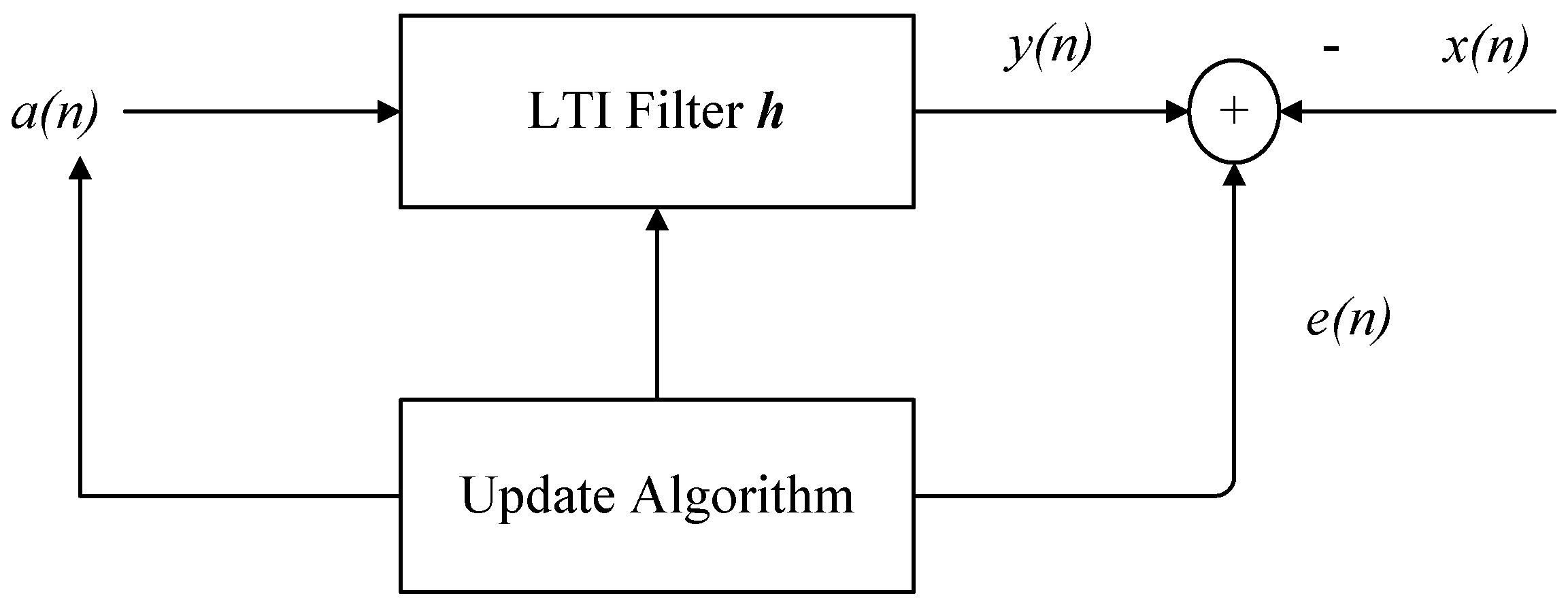
3.3. Matrix Inverse Lemma for Derivation of the Recursive Least-Squares Filter

In many signal processing applications, the data is generated by sampling a continuous-time signal. In this way, more data becomes available as the time progresses. One can either wait for all the available data or process the data iteratively in time. The latter approach requires a recursive (online) approach to update the filter taps. Next, the key role played by the matrix inverse lemma (Woodbury matrix identity) in deriving the least-squares (RLS) filter will be presented.
The matrix inverse lemma states that [12]:
( A + x y H ) 1 = A 1 A 1 x y H A 1 1 + y H A 1 x ,
where matrix A R N × N is assumed invertible, and x , y R N .
Consider now the linear time-invariant (LTI) system shown in Figure 4. The problem is to adapt the m-tap FIR filter coefficients h so that its output y ( n ) follows the reference signal x ( n ) . The received signal y ( n ) is expressed as:
y ( n ) = i = 0 m 1 h n ( i ) a ( n i ) = h n H a n ,
where a n = [ a ( n ) , a ( n 1 ) , , a ( n m + 1 ) ] H is the vector containing the m most recent samples of input signal a ( n ) . Our goal is to estimate the taps of filter h at each time slot n using a least-squares estimation approach. Specifically, the problem resumes to:
h ^ n = arg min h n | | A n h n x n | | 2 2 , n = 1 , 2 , , N ,
where
A n = a ( 1 ) a ( 0 ) a ( m + 2 ) a ( 2 ) a ( 1 ) a ( m + 1 ) a ( n 1 ) a ( n 2 ) a ( n m ) a ( n ) a ( n 1 ) a ( n m + 1 ) = a 1 H a 2 H a n 1 H a n H = A n 1 a n H ,
and
h n = h n ( 0 ) h n ( 1 ) h n ( m 2 ) h n ( m 1 ) and x n = x ( 1 ) x ( 2 ) x ( n 1 ) x ( n ) = x n 1 x ( n ) .
As time evolves the number of rows of matrix A n keeps increasing, and to avoid repeatedly calculating from scratch the least-squares estimate of h ^ n for each instant of time n, expressing h ^ n in terms of h ^ n 1 helps to reduce the computational burden. Indeed, such an approach exhibits the huge benefit of reducing the computational complexity incurred by evaluating the taps of the filter at each time instant.
As we described earlier in (14) and (15), the problem (21) admits the solution
h ^ n = ( A n H A n ) 1 A n H x n .
Setting R n = A n H A n and p n = A n H x n leads to
h ^ n = R n 1 p n .
Moreover, since
R n = A n H A n = i = 1 n a i a i H = i = 1 n 1 a i a i H + a n a n H = R n 1 + a n a n H ,
(22) can be expressed as
h ^ n = ( R n 1 + a n a n H ) 1 p n .
Applying the matrix inverse lemma (19) to the inverse of the matrix contained in Equation (23) yields:
R n 1 = ( R n 1 1 + a n a n H ) 1 = R n 1 1 R n 1 1 a n a n H R n 1 1 1 + a n H R n 1 1 a n .
Furthermore, defining k n = R n 1 1 a n 1 + a n H R n 1 1 a n and Σ n = R n 1 , it follows that
Σ n = Σ n 1 k n a n H Σ n 1 ,
and
Σ n a n = Σ n 1 a n k n a n H Σ n 1 a n = k n ( 1 + a n H Σ n 1 a n ) k n a n H Σ n 1 a n = k n .
Plugging (25) and (26) into (22) results in
h ^ n = Σ n p n = Σ n [ p n 1 + a n x ( n ) ] = Σ n p n 1 + Σ n a n x ( n ) = ( Σ n 1 k n a n H Σ n 1 ) p n 1 + k n x ( n ) = h ^ n 1 k n a n H h ^ n 1 + k n x ( n ) = h ^ n 1 + k n [ x ( n ) a n H h ^ n 1 ] = h ^ n 1 + ϵ ( n ) k n ,
where ϵ ( n ) = x ( n ) a n H h ^ n 1 and the second equality comes from the fact that
p n = A n H x n = A n 1 H x n 1 + a n x ( n ) = p n 1 + a n x ( n ) .
In a nutshell, the RLS algorithm can be summarized as follows:
(1)
Choose a large positive number α, and initialize Σ 0 = α I and h ^ 0 = 0 .
(2)
For n = 1 , 2 , , N , sequentially update
k n = Σ n 1 a n 1 + a n H Σ n 1 a n , ϵ ( n ) = x ( n ) a n H h ^ n 1 , h ^ n = h ^ n 1 + ϵ ( n ) k n , Σ n = Σ n 1 k n a n H Σ n 1 .
As the algorithm processes, the error made by approximating Σ 0 = α I and h ^ 0 = 0 becomes less and less significant [12].
In some cases, a weighted least squares estimation error is used as the minimizer by multiplying the error terms with so-called “forgetting factors”, which are intended to reduce the influence of old data [14]. The RLS algorithm has emerged as a powerful tool for adaptive filtering, prediction and system identification applications. Despite the fundamental role played by the RLS algorithm in the adaptive signal processing field, it encounters numerical problems when implemented in a finite precision environment, and especially in fixed-point arithmetic DSP processors [15]. The round-off error propagation, defined as the influence of subsequent computations when a single perturbation occurs at a random iteration, represents one of the major drawbacks of the RLS algorithm in a finite precision implementation and has been well studied in literature [16,17,18]. A popular method to improve the accuracy and stability of RLS algorithm is to implement a variable forgetting factor (VFF) [19,20,21]. Other modified RLS methods can be found in [22,23,24,25] and the references therein.

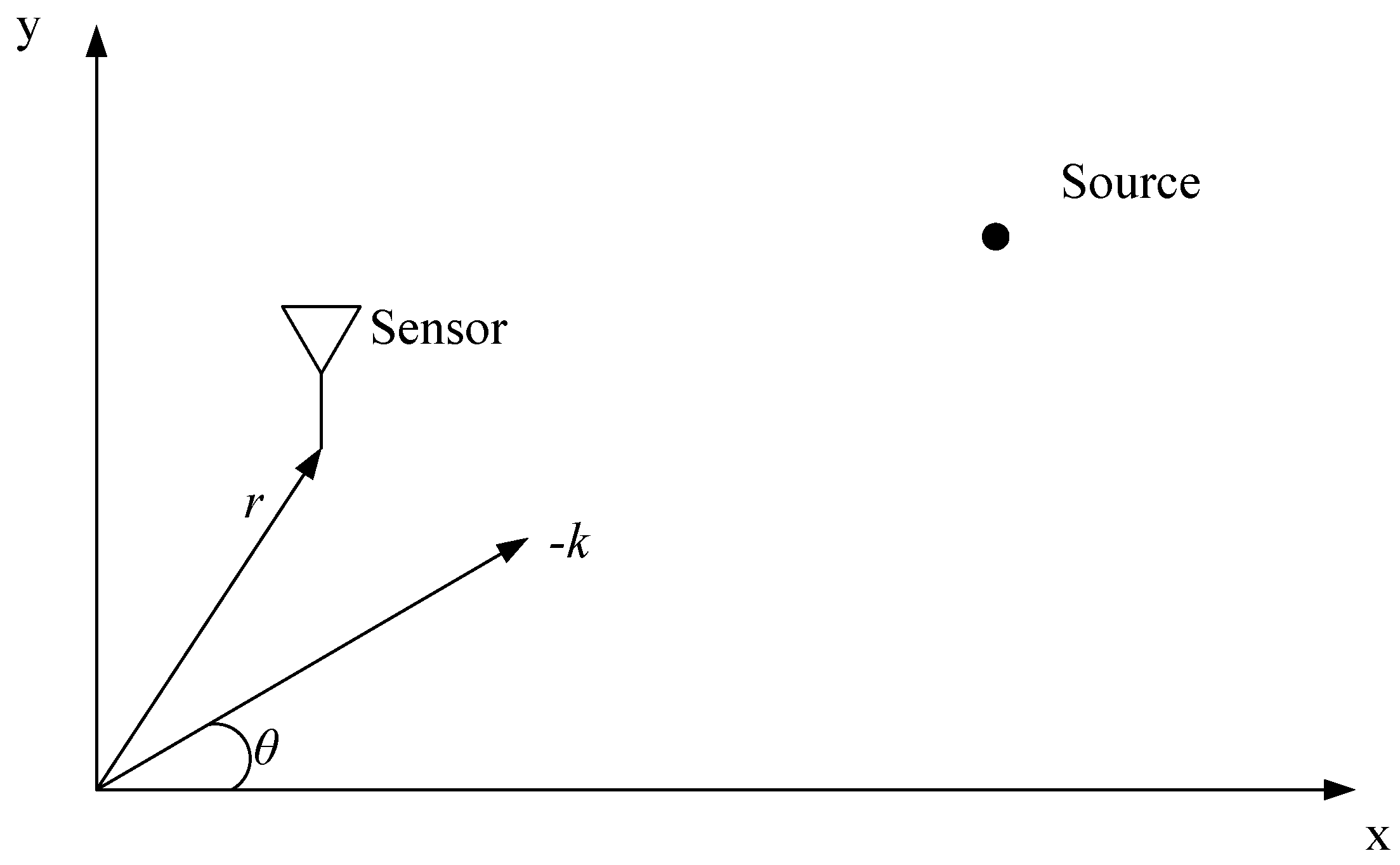
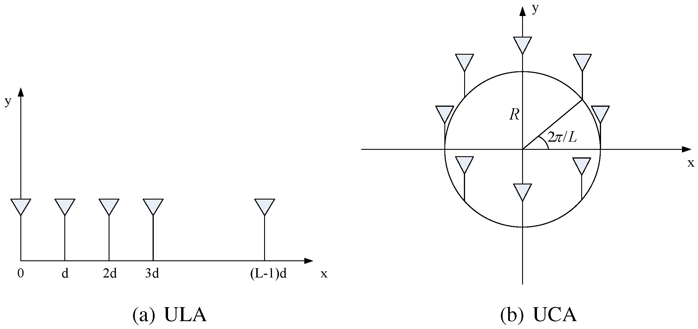
3.4. Matrix Theory in Sensor Array Signal Processing

Sensor array signal processing focuses mainly on signal enumeration and source location applications, and presents a huge importance in many domains such as radar, sonar and underwater surveillance. The classic problem in sensor array signal processing is to detect and locate the radiating sources given the temporal and spatial information collected from the sensors. The goal of this section is to introduce the basic framework of sensor array signal processing and illustrate the fundamental role of matrix theory in representing and addressing the detection and estimation problems associated with the radiating sources.
First consider the one-source-one-sensor scenario shown in Figure 5. It is proved in [26] that under the far-field and narrowband assumptions, the output of a sensor can be modeled as follows:
x ( t ) = g ( θ ) s ( t ) e j r T k ,
where g ( θ ) is a function of the direction of arrival (DOA) θ, and it represents the frequency response of the sensor. Variable s ( t ) represents the complex envelope of the source signal, and r and k stand for the radius vector and the wave vector, respectively. The magnitude of k is defined as | k | = α = 2 π / λ , where λ is the wavelength. As shown in Figure 5, in a two-dimensional plane, we have k = α ( cos θ , sin θ ) T and r = ( x , y ) T . Thus, the output of the sensor can be simplified to
x ( t ) = g ( θ ) e j α ( x cos θ + y sin θ ) s ( t ) = a ( θ ) s ( t ) ,
where a ( θ ) = g ( θ ) e j α ( x cos θ + y sin θ ) .
For the one-source-L-sensor case, the array output vector can be expressed as
x ( t ) = a ( θ ) s ( t ) ,
where x ( t ) = [ x 1 ( t ) , x 2 ( t ) , , x L ( t ) ] T denotes the output of each sensor and a ( θ ) = [ a 1 ( θ ) , a 2 ( θ ) , , a L ( θ ) ] T stands for the steering vector and captures the sensor array geometry information. Two common array geometries, termed as the uniform linear array (ULA) and uniform circular array (UCA), are depicted in Figure 6. For ULA, r l = [ ( l 1 ) d , 0 ] T , and for UCA, r l = R [ cos ( 2 π ( l 1 ) / L ) , sin ( 2 π ( l 1 ) / L ) ] T . Additionally, if we assume that all the sensors have the same frequency response, g 1 ( θ ) = = g L ( θ ) = g ( θ ) , the ULA steering vector takes the form:
a ULA ( θ ) = g ( θ ) [ 1 , e j α d cos θ , , e j α ( L 1 ) d cos θ ] T ,
and the UCA admits the form:
a UCA ( θ ) = g ( θ ) [ e j α R cos θ , e j α R [ cos ( 2 π / L ) cos θ + sin ( 2 π / L ) sin θ ] , , e j α R [ cos ( 2 π ( L 1 ) / L ) cos θ + sin ( 2 π ( L 1 ) / L ) sin θ ] ] T .
Furthermore, if N source signals with DOA θ n , n = 1 , 2 , , N , are superimposed on an L-dimensional array (N-source-L-sensor), the array output vector can be expressed as
x ( t ) = n = 1 N a ( θ n ) s n ( t ) ,
or compactly as
x ( t ) = A ( θ ) s ( t ) ,
where x ( t ) = [ x 1 ( t ) , , x L ( t ) ] T R L , A ( θ ) = [ a ( θ 1 ) , , a ( θ N ) ] R L × N and s ( t ) = [ s 1 ( t ) , , s N ( t ) ] T R N . In the presence of an additive noise ν ( t ) , the sensor array equation can be expressed as:
x ( t ) = A ( θ ) s ( t ) + ν ( t ) .
The central goal of array signal processing is to locate the source signals, or equivalently, to estimate the DOAs θ given the observed data x ( t ) at the sensors. From (33), we can see that the input and the output are just related by a steering matrix A ( θ ) and the problem formulation is simplified using a steering matrix representation. Moreover, the estimation problem may also be addressed efficiently by exploring the special structure of the steering matrix. For instance, under the ULA geometry, we aim at estimating θ = [ θ 1 , , θ N ] T subject to
x 1 ( t ) x 2 ( t ) x L ( t ) = 1 1 1 e j α d cos θ 1 e j α d cos θ 2 e j α d cos θ N e j α ( L 1 ) d cos θ 1 e j α ( L 1 ) d cos θ 2 e j α ( L 1 ) d cos θ N s 1 ( t ) s 2 ( t ) s N ( t ) + ν 1 ( t ) ν 2 ( t ) ν L ( t ) .
It can be observed that the steering matrix A ( θ ) for the ULA geometry is a Vandermonde matrix. Thus, the special properties of Vandermonde matrices can be exploited to develop efficient algorithms to estimate the DOA. For instance, the estimation of signal parameters by rotation invariant techniques (ESPRIT) [27] utilizes the so-called shifting property of Vandermonde matrices, which can be easily understood by considering two submatrices A 1 and A 2 of A ( θ ) , obtained by removing the first and last rows of the steering matrix A ( θ ) , respectively. Due to the structure of Vandermonde matrix A ( θ ) in (34), the shifting property manifests through the fact that matrices A 1 and A 2 are related by means of shift matrix Φ via A 2 = A 1 Φ , where Φ is a diagonal matrix with diagonal elements [ e j α d cos θ 1 , e j α d cos θ 2 , , e j α d cos θ N ] . Therefore, the DOA estimation problem is simplified to that of finding Φ, which can be addressed by exploring the eigenvalue decomposition of the sensor array covariance matrix. The interested reader is referred to [14,26,28] for more details about ESPRIT and other matrix factorization based algorithms for sensor array estimation.

3.5. Random Matrix Theory in Signal Estimation and Detection

Suppose we are given a parameter to be estimated with a “population size” of N and n observations of the population. Many estimation methods proposed in literature rely on the asymptotic behavior that the number of observations is much larger than the population size, i.e., n / N . However, in modern signal processing, this assumption sometimes is not met in practice. For instance, in biological networks, the estimate generally consists of a large number of DNAs and the population size may also grow as the number of observations increases. Moreover, in radar applications, a large number of sensors are used to detect a fast moving object with observations available only during a short time period. Therefore, under such a set-up, the proposed estimators may perform poorly if the condition n / N is not satisfied. Recently, a novel estimation method based on the large dimensional random matrix theory has been proposed to cope with this situation. The random matrix theory originated from the work of Wigner [29] in 1955 and was later generalized to a large extent by Marcenko and Pastur [30] in 1967. Recently, a considerable amount of work based on random matrix theory has emerged in the literature of signal processing, wireless communications and information theory.
Consider a simple example from [31], where x C N is a complex random vector with zero mean and covariance matrix R . Given n observations of x , we will consider a classic estimator of R in the form of the sample covariance matrix R n = 1 n i = 1 n x i x i H . Because of the law of large numbers, | | R n R | | 2 a . s . 0 as n , where | | · | | 2 denotes the spectral norm of a matrix, i.e., the absolute value of the largest eigenvalue if the matrix is Hermitian, and a . s . stands for almost sure convergence. By taking the special case where R = I N , it was shown in [31] that if n but n / N does not tend to zero, i.e., n / N = 1 / 2 , the spectral norm of R n I N is at least greater than 1. The problem lies in the fact that the random eigenvalue distribution F R n of R n does not converge to a Dirac mass measure at 1 [31]. However, it is observed that in many scenarios, it converges to a limit distribution as N , n , N / n = c . In the special case where R = I N , the limit distribution is referred to as the Marcenko-Pastur distribution [30]. The derivation of the eigenvalue distribution for such large dimensional matrices brings the most fundamental tool of random matrix theory, namely the Stieltjes transform, and it is also a necessary prior step for parameter estimation and detection problems. Furthermore, the knowledge of the eigenvalue distribution for large dimensional matrices alone plays a paramount role in some wireless communication problems, such as computing or approximating the capacity of multi-antenna based channels. The interested reader can refer to [32,33,34,35] for more details about applications of random matrix theory in wireless communications.
In the following, we present a parameter estimation problem where the conventional sample covariance method fails for comparable population size and number of observations. In this case, an estimation method based on the spectral properties of large dimensional random matrices, referred to as the G-estimation method [36] can be employed to improve the performance. Rather than analyzing the complicated mathematical details of the random matrix theory and G-estimation method, our aim is instead to illustrate how the random matrix theory can be applied in a typical application. Consider a multi-source power estimation problem [31], where at time t, a number of N sensors receive signals from K sources which are equipped with n 1 , n 2 , , n K transmitters, respectively. The observed data y C N from sensors at time t can be expressed as
y ( t ) = k = 1 K P i U ˜ i x i ( t ) + σ ν ( t ) ,
where P i denotes the transmit power of source i, x i C n i stands for the signal collected from source i and it is assumed to be complex Gaussian distributed with zero mean and identity covariance matrix, and σ ν represents the additive noise. For simplicity, the channel matrix U ˜ i C N × n i is selected such that [ U ˜ 1 , U ˜ 2 , , U ˜ K ] C N × ( n 1 + n 2 + + n K ) represent the n 1 + n 2 + + n K columns of the unitary matrix U C N × N .
If follows that
E [ y ( t ) y ( t ) H ] = U P U H + σ 2 I N ,
where P is a diagonal matrix with diagonal elements
P 1 , , P 1 n 1 , P 2 , , P 2 n 2 , , P K , , P k n K , 0 , , 0 N n 1 n K .
Suppose that L independent observations of y ( t ) are available, i.e., y ( 1 ) , y ( 2 ) , , y ( L ) . Thus, it follows that as L :
1 L i = 1 L y ( i ) y ( i ) H σ 2 I N U P U H a . s . 0 ,
and a consistent estimator can be derived. However, when N is also a large number and L and N are comparable, (36) does not hold anymore. Using the Stieltjes transform and its extensions, the G-estimation method is generally adopted to improve the estimation performance. More technical and mathematical details about the Stieltjes transform and its generalizations can be found in [31,35].

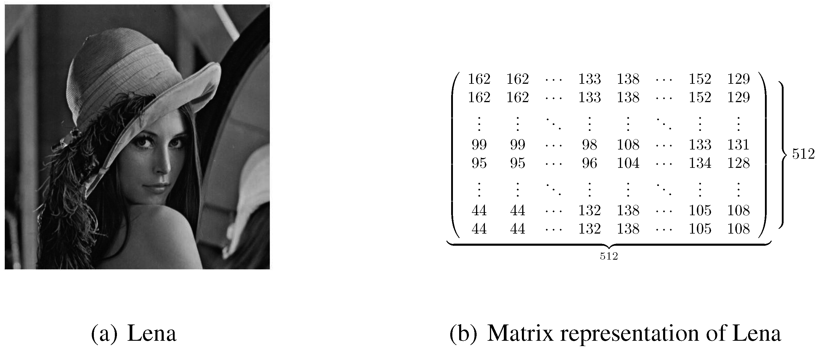
4. Matrices in Image Processing

In digital image processing, images are usually represented using matrices. For example, the gray-scale image “Lena.tiff” is illustrated in Figure 7a, while its matrix representation is shown in Figure 7b. A matrix element is called “pixel”. Most digital images use integer numbers between 0 (to indicate black) and 255 (to indicate white) to represent the values of pixels, giving a total of 2 8 = 256 gray levels. Color images, in turn, can be represented by three matrices. These matrices specify the amount of red (R), green (G) and blue (B) present in the image. This representation system is known as the RGB system.
In the following sections, two image compression methods are discussed, namely the block transform coding and wavelet representation, both of which decompose the image matrix into several submatrices and use the sparsity of these submatrices to compress the image.

4.1. Block Transform Coding

The block transform coding [37] is a compression technique which divides an image into several non-overlapping subimages of equal size and then processes these subimages using a 2-D transform. It turns out that after implementing a block transformation, for most subimages, a large portion of the resulting coefficients present small magnitudes and thus can be discarded. Therefore, using the block transform coding, one can develop a very simple storage mechanism since most of the block transformed entries assume small values and can be neglected.
Specifically, an M × N image is divided into M N / n 2 subimages each of which has a size n × n . Consider a subimage with coefficients g ( x , y ) , the 2-D transform can be expressed as follows:
T ( u , v ) = x = 0 n 1 y = 0 n 1 g ( x , y ) r ( x , y , u , v ) .
The original image g ( x , y ) can be recovered by the inverse transform defined by
g ( x , y ) = u = 0 n 1 v = 0 n 1 T ( u , v ) s ( x , y , u , v ) .
In these equations, r ( x , y , u , v ) and s ( x , y , u , v ) are referred to as forward and inverse transformation kernels, respectively. The kernels depend on what transformation (DFT, DCT, Haar Wavelet Transform, etc.) is implemented. In this paper, the JPEG image compression standard using the discrete cosine transform (DCT) is presented. In this case, we have
r ( x , y , u , v ) = s ( x , y , u , v ) = α ( u ) α ( v ) cos ( 2 x + 1 ) u π 2 n cos ( 2 y + 1 ) v π 2 n ,
where
α ( x ) = 1 n , x = 0 , 2 n , x = 1 , 2 , , n 1 .
Equations (37) and (38) can be written in a compact form by using matrices. Consider (38) as an example,
G = u = 0 n 1 v = 0 n 1 T ( u , v ) S u v ,
where G is the subimage matrix consisting of g ( x , y ) and
S u v = s ( 0 , 0 , u , v ) s ( 0 , 1 , u , v ) s ( 0 , n 1 , u , v ) s ( 1 , 0 , u , v ) s ( 1 , 1 , u , v ) s ( 1 , n 1 , u , v ) s ( n 1 , 0 , u , v ) s ( n 1 , 1 , u , v ) s ( n 1 , n 1 , u , v ) .
Similarly, (37) can be defined as
T = x = 0 n 1 y = 1 n 1 g ( x , y ) R x y .

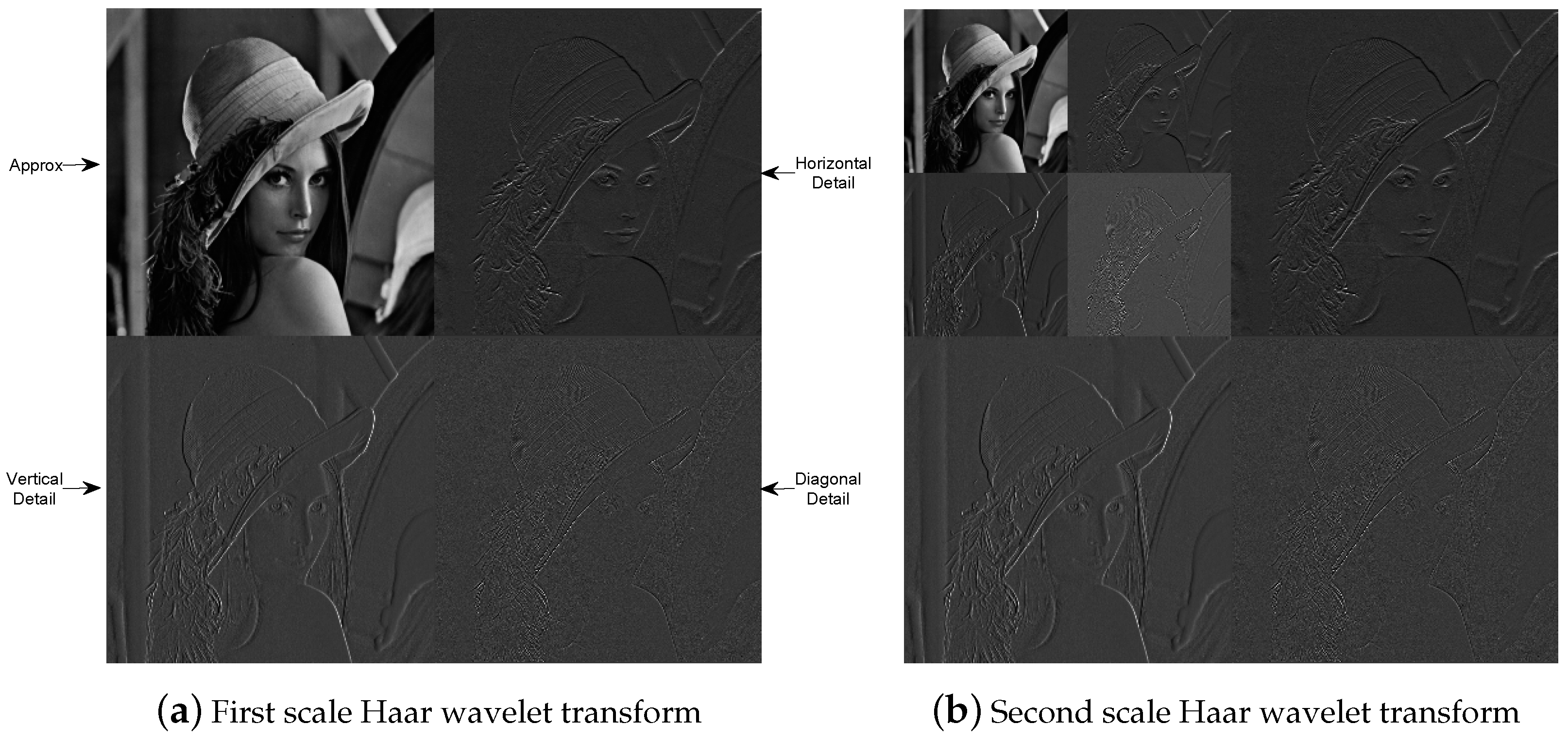
4.2. Wavelet Representation

Besides the classical DCT image representation, another modern image representation method, that relies on the 2-D wavelet coding and lies at the basis of JPEG 2000 standard [37], is used extensively. Different from the transform coding, the wavelet coding processes the whole image and results in a modified image consisting of four subimages. For example, after processing Figure 7a using the Haar wavelet, the modified image in Figure 8a is obtained. The four submatrices represent the approximation, the horizontal details, the vertical details and the diagonal details, respectively. One can observe that the three detail matrices can be coarsely quantized since their coefficients roughly present similar values. Moreover, the approximation matrix in Figure 8a can also be decomposed into four sub-subimages as shown in the upper left corner of Figure 8b. In this way, the image is compressed to a higher degree given the premise that the original image can be recovered with a tolerated quality.

5. Compressive Sensing

The celebrated Shannon/Nyquist sampling theorem states that in order to reconstruct a signal without losing information, the sample rate must be at least two times larger than the signal bandwidth. So far, most signal acquisition techniques rely on this principle. As mentioned in Section 4.1, transform coding plays a key role in data acquisition systems. However, this compression framework suffers from several drawbacks [38]. For instance, consider a discrete signal x R N with entries x [ n ] , n = 0 , 1 , , N 1 . An image or a higher-dimensional data structure can be also vectorized into a long one-dimensional vector. It is known that any signal in R N can be represented in terms of a basis of N vectors { ψ i } i = 0 N 1 . In this case,
x = i = 0 N 1 s i ψ i = Ψ s ,
where s stands for the weighting coefficients and Ψ is the basis matrix with columns [ ψ 0 , , ψ N 1 ] . The signal x is called K-sparse if only K coefficients of s are non-zero and the remaining N K coefficients are roughly zero (or can be truncated to zero). Thus, in order to process the transform coding, the locations of the K non-zero coefficients must be coded, which results in an overhead. Moreover, the N K zero coefficients still need to be computed even though they will be discarded.
Compressive sensing addresses these issues by directly processing the compressed signal without acquiring the original N-sample signal provided that the signal is K-sparse [39]. This novel sampling method dramatically undersamples the signal at a greatly reduced rate. Next we will present the mathematical model behind this new technique.
Consider the following representation [38]:
y = Φ x = Φ Ψ s = Θ s ,
where x R N stands for the original signal, y R M ( M N ) denotes the compressed signal, and Φ R M × N represents the linear measurement process. Mathematically, the problem can be formulated as follows. First, find a matrix Φ such that y = Φ x preserves most of the information embedded in x . Second, find an algorithm to recover x from only M samples of y .

5.1. Good Sensing Matrices

The most critical issue is to determine whether Φ is good for compressive sensing and reconstruction. The reconstruction seems to be impossible at first glance since the problem is ill-conditioned ( M < N ). However, it is now well-known that one can reconstruct the sparse signal from a limited number of measurements if the sensing matrix satisfies the restricted isometry property (RIP) [39,40,41]. A matrix Φ R M × N is said to satisfy the RIP of order K < M with isometry constant δ K ( 0 , 1 ) if
( 1 δ K ) | | v | | 2 2 | | Φ v | | 2 2 ( 1 + δ K ) | | v | | 2 2
holds for any K-sparse vector v .
Since verifying the RIP property of a matrix requires an exhaustive search of all N K possibilities, most algorithms developed so far are based on randomization. Typically, the matrix elements are produced by independent and identically distributed (i.i.d.) random variables with certain distribution. References [42] and [43] proved that if the elements of matrix Φ are i.i.d. Gaussian random variables with zero means and variance 1 / N , and M c K log ( N / K ) where c is a small constant, then Φ satisfies RIP with a very high probability. Therefore, the signal can be recovered from only M c K log ( N / K ) N variables. Other available selections for robust sensing matrices are discussed in [42,44].

5.2. Compressive Signal Reconstruction

The signal reconstruction problem requires the recovery of signal x , or equivalent of the weighted coefficients s , given the sensing matrix Φ, basis matrix Ψ and compressed signal y . The ultimate goal of compressive sensing is to find the possible sparsest representation of the signal. Therefore, the ideal reconstruction problem can be expressed via the l 0 norm as follows:
min | | s | | 0 s . t . Θ s = y .
Unfortunately, such a formulation of the problem is both numerically unstable and computationally complex (NP-complete) [45]. For simplicity, problem (44) can be reduced to minimize the l 2 norm of s
min | | s | | 2 s . t . Θ s = y ,
which leads to the closed form solution s ^ = θ T ( θ θ T ) 1 y . However, this method will almost never yield a K-sparse solution. Even worse, usually a full representation solution (no zero elements) will be generated by using the l 2 norm.
Surprisingly, the optimization based on the l 1 norm is the most promising recovery technique used so far for sparse signals. In this case, the recovery problem is formulated as follows:
min | | s | | 1 s . t . Θ s = y .
In some cases, the l 1 minimization yields the same result as the ideal l 0 minimization [46]. Moreover, the l 1 minimization can be efficiently solved via linear programming which presents a computational complexity of O ( N 3 ) . For the last decade, a series of papers [39,43,47] explained why l 1 minimization can be approximated as an l 0 minimization and why it can recover a sparse signal. Until now, most of the works dedicated to compressive sensing, see, e.g., the works of Dandes, Romberg, Tao and Donoho [39,40,41,42,43] assume the l 1 norm formulation.

6. Conclusions

This paper overviewed how matrix theory can be applied in wireless communications and signal processing applications. In particular, this paper illustrated how matrix transformations, matrix decompositions and random matrix theory could be exploited in the implementation, characterization and optimization of MIMO communication systems, OFDM signaling schemes and signal estimation applications. This paper also reviewed the significant role played by matrices in representing and processing digital images and signals acquired by an array of sensors. Furthermore, a recent research activity termed as compressive sensing was briefly discussed herein paper. It will require continued efforts from researchers in wireless communications and signal processing to ultimately exploit the full potential applications of matrix theory. Furthermore, the complex phenomena in nature and engineering applications require higher-dimensional matrices for their modeling, characterization and understanding. In this regard, tensors have been used in mathematics, physics and engineering since they are a generalization of scalars, vectors and two-dimensional arrays to represent more complex quantities and properties in higher dimensions. Therefore, a promising research direction is to investigate new applications of tensors in wireless communications and signal processing, and to extend the arsenal of mathematical tools available for storing, extracting and processing information from tensors. Finally, we would like to mention that linear algebra plays a very important role in developing powerful algorithms in bioinformatics and systems biology applications. Numerous algorithms for the inference of gene and proteomic regulatory networks as well as for the inference of transcription factor networks have been proposed in literature (see, e.g., [48,49]) by exploiting linear algebra tools. However, reviewing these computational biology applications as well as numerous other machine learning applications where linear algebra plays a key role is beyond the scope of this paper.

Acknowledgments

This work was supported by NSF Award CCF-1318338.

Author Contributions

Xu Wang contributed to draft writing. Erchin Serpedin proposed the framework of the paper and helped to improve the manuscript. All authors read and approved the manuscript.

Conflicts of Interest

The authors declare no conflict of interest.

References

  1. Shannon, C.E. A mathematical theory of communication. Bell Syst. Tech. J. 1948, 27, 379–423. [Google Scholar] [CrossRef]
  2. Introduction to LTE-Advanced: Application Note. Agilent Technol. 2011. Available online: http://cp.literature.agilent.com/litweb/pdf/5990-6706EN.pdf (accessed on 6 January 2016).
  3. Telatar, E. Capacity of multi-antenna Gaussian channels. Eur. Trans. Telecommun. 1999, 10, 585–596. [Google Scholar] [CrossRef]
  4. Goldsmith, A. Wireless Communications; Cambridge University Press: Cambridge, UK, 2005. [Google Scholar]
  5. Foschini, G.J. Layered space-time architecture for wireless communication in fading environments when using multi-element antennas. Bell Labs Tech. J. 1996, 1, 41–59. [Google Scholar] [CrossRef]
  6. Foschini, G.J.; Gans, M.J. On limits of wireless communications in fading environment when using multiple antennas. Wirel. Pers. Commun. 1998, 6, 311–335. [Google Scholar] [CrossRef]
  7. Goldsmith, A.; Jafar, S.A.; Jindal, N.; Vishwanath, S. Capacity limits of MIMO channels. IEEE J. Sel. Areas Commun. 2003, 21, 684–702. [Google Scholar] [CrossRef]
  8. Wang, X.; Serpedin, E.; Qaraqe, K. A variational approach for assessing the capacity of a memoryless nonlinear MIMO channel. IEEE Commun. Lett. 2014, 18, 1315–1318. [Google Scholar] [CrossRef]
  9. Gray, R.M. Toeplitz and Circulant Matrices: A Review; Now Publishers Inc.: Norwell, MA, USA, 2006. [Google Scholar]
  10. Bolcskei, H.; Zurich, E. MIMO-OFDM wireless systems: Basics, perspectives, and challenges. IEEE Trans. Wirel. Commun. 2006, 13, 31–37. [Google Scholar]
  11. Golub, G.H.; VanLoan, C.F. Matrix Computations; The Johns Hopkins University Press: Baltimore, MA, USA, 1996. [Google Scholar]
  12. Kay, S. Fundamentals of Statistical Signal Processing: Estimation Theory; Prentice Hall: Upper Saddle River, NJ, USA, 1993. [Google Scholar]
  13. Reilly, J.P. Matrix Computations in Signal Processing: Lecture Notes; Electrical and Computer Engineering Department, McMaster University: Hamilton, ON, Canada, 24 September 2006. [Google Scholar]
  14. Haykin, S. Array Signal Processing; Prentice Hall: Upper Saddle River, NJ, USA, 1985. [Google Scholar]
  15. Paleologu, C.; Ciochina, S.; Enescu, A. A family of recursive least-squares adaptive algorithms suitable for fixed-point implementation. Int. J. Adv. Telecommun. 2009, 2, 88–97. [Google Scholar]
  16. Liavas, A.; Regalia, P. On the numerical stability and accuracy of the conventional recursive least squares algorithm. IEEE Trans. Signal Process. 1999, 47, 88–96. [Google Scholar] [CrossRef]
  17. Ljung, S.; Ljung, L. Error propagation properties of recursive least-squares adaptation algorithms. Automatica 1985, 21, 157–167. [Google Scholar] [CrossRef]
  18. Verhaegen, M. Round-off error propagation in four generally-applicable, recursive, least-squares estimation schemes. Automatica 1989, 25, 437–444. [Google Scholar] [CrossRef]
  19. Bhotto, Z.; Antoniou, A. New improved recursive least-squares adaptive-filtering algorithms. IEEE Trans. Circuits Syst. I Reg. Pap. 2013, 60, 1548–1558. [Google Scholar] [CrossRef]
  20. Leung, S.; So, C. Gradient-based variable forgetting factor RLS algorithm in time-varying environments. IEEE Trans. Signal Process. 2005, 53, 3141–3150. [Google Scholar] [CrossRef]
  21. Paleologu, C.; Benesty, J.; Ciochina, S. A robust variable forgetting factor recursive least-squares algorithm for system identification. IEEE Signal Process. Lett. 2008, 15, 597–600. [Google Scholar] [CrossRef]
  22. Ardalan, S. Floating-point roundoff error analysis of the exponentially windowed RLS algorithm for time-varying systems. IEEE Trans. Circuits Syst. 1986, 33, 1192–1208. [Google Scholar] [CrossRef]
  23. Bottomley, G.; Alexander, S. A novel approach for stabilizing recursive least squares filters. IEEE Signal Process. Lett. 1991, 39, 1770–1779. [Google Scholar] [CrossRef]
  24. Chansakar, M.; Desai, U. A robust recursive least squares algorithm. IEEE Signal Process. Lett. 1997, 45, 1726–1735. [Google Scholar] [CrossRef]
  25. Haykin, S. Adpative Filtering Theory; Prentice Hall: Upper Saddle River, NJ, USA, 2002. [Google Scholar]
  26. Krim, H.; Viberg, M. Two decades of array signal processing research. IEEE Signal Process. Mag. 1996, 13, 67–94. [Google Scholar] [CrossRef]
  27. Roy, R.; Kailath, T. ESPRIT-estimation of signal parameters via rotational invariance techniques. IEEE Trans. Acoust. Speech Signal Process. 1989, 37, 984–995. [Google Scholar] [CrossRef]
  28. Stoica, P.; Moses, R.L. Introduction to Spectral Analysis; Prentice Hall: Upper Saddle River, NJ, USA, 1997. [Google Scholar]
  29. Wigner, E. Characteristic vectors of bordered matrices with infinite dimensions. Ann. Math. 1955, 62, 548–564. [Google Scholar] [CrossRef]
  30. Marcenko, V.A.; Pastur, L.A. Distributions of eigenvalues for some sets of random matrices. Math. USSR-Sbornik 1967, 1, 457–483. [Google Scholar] [CrossRef]
  31. Couillet, R.; Debbah, M. Signal processing in large systems: A new paradigm. IEEE Signal Process. Mag. 2003, 30, 24–39. [Google Scholar] [CrossRef]
  32. Couillet, R.; Debbah, M.; Siverstein, J.W. A deterministic equivalent for the analysis of correlated MIMO multiple access channels. IEEE Trans. Inf. Theory 2011, 57, 3493–3514. [Google Scholar] [CrossRef]
  33. Dupuy, F.; Loubaton, P. On the capacity achieving covariance matrix for frequency selective MIMO channels using the asymptotic approach. IEEE Trans. Inf. Theory 2011, 57, 5737–5753. [Google Scholar] [CrossRef] [Green Version]
  34. Couillet, R.; Debbah, M. Random Matrix Methods for Wireless Communications; Cambridge University Press: Cambridge, UK, 2011. [Google Scholar]
  35. Tulino, M.A.; Verdu, S. Random Matrix Theory and Wireless Communications; Now Publishers: Norwell, MA, USA, 2004. [Google Scholar]
  36. Girko, V.L. Theory of Random Determinants; Kluwer Academic Publisher: Dordrecht, The Netherlands, 1990. [Google Scholar]
  37. Gonzalez, R.C.; Woods, R.E. Digital Image Processing; Prentice Hall: Upper Saddle River, NJ, USA, 2007. [Google Scholar]
  38. Baraniuk, R.G. Compressive Sensing. IEEE Signal Process. Mag. 2007, 24, 119–121. [Google Scholar] [CrossRef]
  39. Dandes, E.; Romberg, J.; Tao, T. Robust uncertainty principles: Exact signal reconstruction from highly incomplete frequency information. IEEE Trans. Inf. Theory 2006, 52, 489–509. [Google Scholar]
  40. Dandes, E.; Romberg, J. Quantitative robust uncertainty principles and optimally sparse decompositions. Found. Comput. Math. 2006, 6, 227–254. [Google Scholar]
  41. Candes, E.; Tao, T. Decoding by linear programming. IEEE Trans. Inf. Theory 2005, 51, 4203–4215. [Google Scholar] [CrossRef]
  42. Candes, E.; Tao, T. Near optimal signal recovery from random projections: Universal encoding strategies? IEEE Trans. Inf. Theory 2006, 51, 5406–5425. [Google Scholar] [CrossRef]
  43. Donoho, D.L. For most large underdetermined systems of equations, the minimal l1-norm near-solution approximates the sparsest near-solution. Commun. Pure Appl. Math. 2004, 59, 797–829. [Google Scholar] [CrossRef]
  44. Baraniuk, R.G.; Davenport, M.A.; DeVore, R.A.; Wakin, M.B. A simple proof of the restricted isometry property for random matrices. Constr. Approx. 2008, 28, 253–263. [Google Scholar] [CrossRef]
  45. Natarajan, B.K. Sparse approximate solutions to linear systems. SIAM J. Comput. 1995, 24, 227–234. [Google Scholar] [CrossRef]
  46. Holtz, H.V. Compressive sensing: A paradigm shift in signal processing. 2008; arXiv:0812.3137. [Google Scholar]
  47. Donoho, D.L.; Huo, X. Uncertainty principles and ideal atomic decomposition. IEEE Trans. Inf. Theory 2001, 47, 2845–2862. [Google Scholar] [CrossRef]
  48. Wang, X.; Alshawaqfe, M.; Dang, X.; Wajid, B.; Noor, A.; Qaraqe, M.; Serpedin, E. An overview of NCA-based algorithms for transcriptional regulatory network inference. Microarrays 2015, 4, 596–617. [Google Scholar] [CrossRef] [PubMed]
  49. Noor, A.; Serpedin, E.; Nounou, M.; Nounou, H. An overview of the statistical methods for inferring gene regulatory networks and protein-protein interaction networks. Adv. Bioinform. 2013, 2013, 953814. [Google Scholar] [CrossRef] [PubMed]
Figure 1. Multiple-input multiple-output (MIMO) channel.
Algorithms 09 00068 g001
Figure 2. Parallel decomposition.
Algorithms 09 00068 g002
Figure 3. Orthogonal frequency-division multiplexing (OFDM).
Algorithms 09 00068 g003
Figure 4. RLS filter.
Algorithms 09 00068 g004
Figure 5. One-sensor one-source array.
Algorithms 09 00068 g005
Figure 6. Array geometries.
Algorithms 09 00068 g006
Figure 7. Example of gray-scale figure.
Algorithms 09 00068 g007
Figure 8. Haar Wavelet transform.
Algorithms 09 00068 g008

