
A Variable Block Insertion Heuristic for the Blocking Flowshop Scheduling Problem with Total Flowtime Criterion

Abstract
:1. Introduction
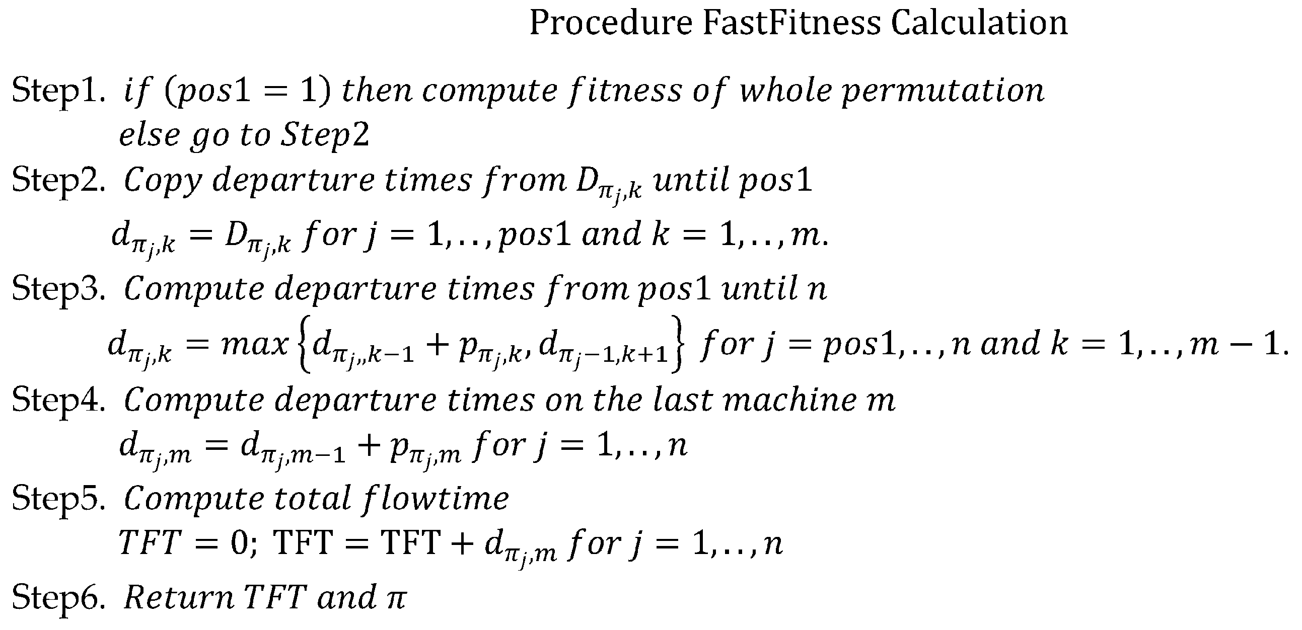
2. Blocking Flow Shop Scheduling Problem
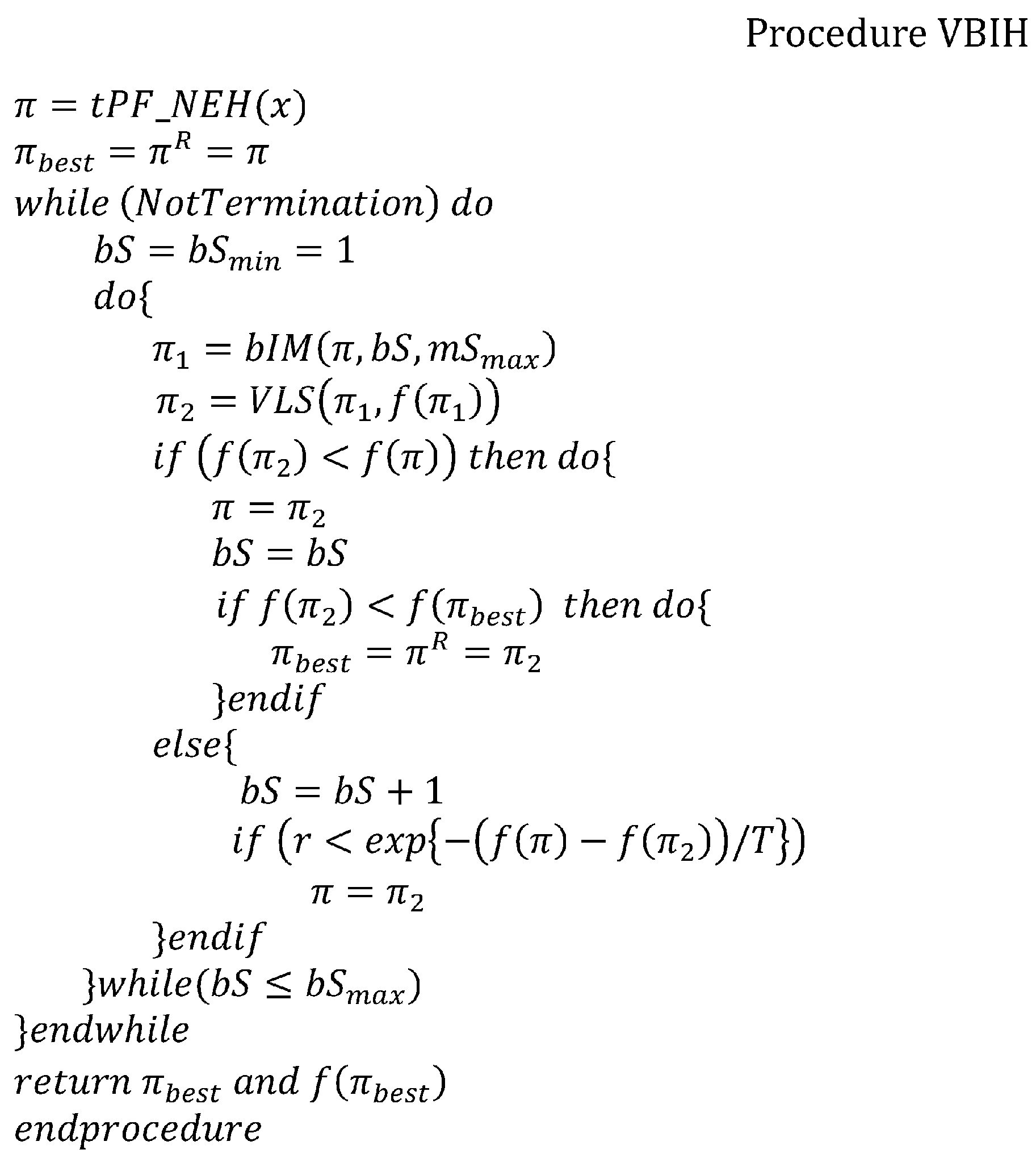
3. Variable Block Insertion Heuristic
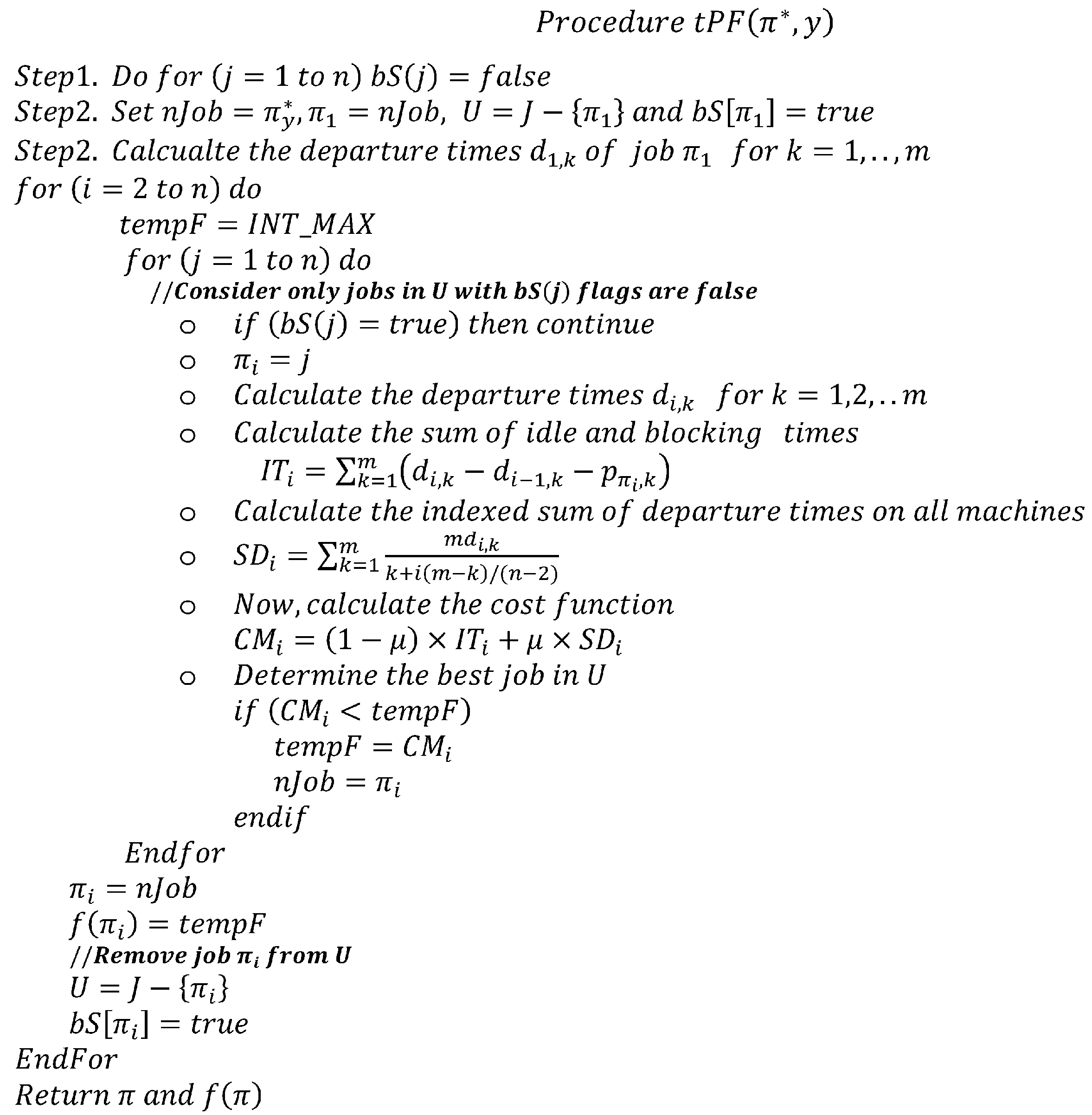
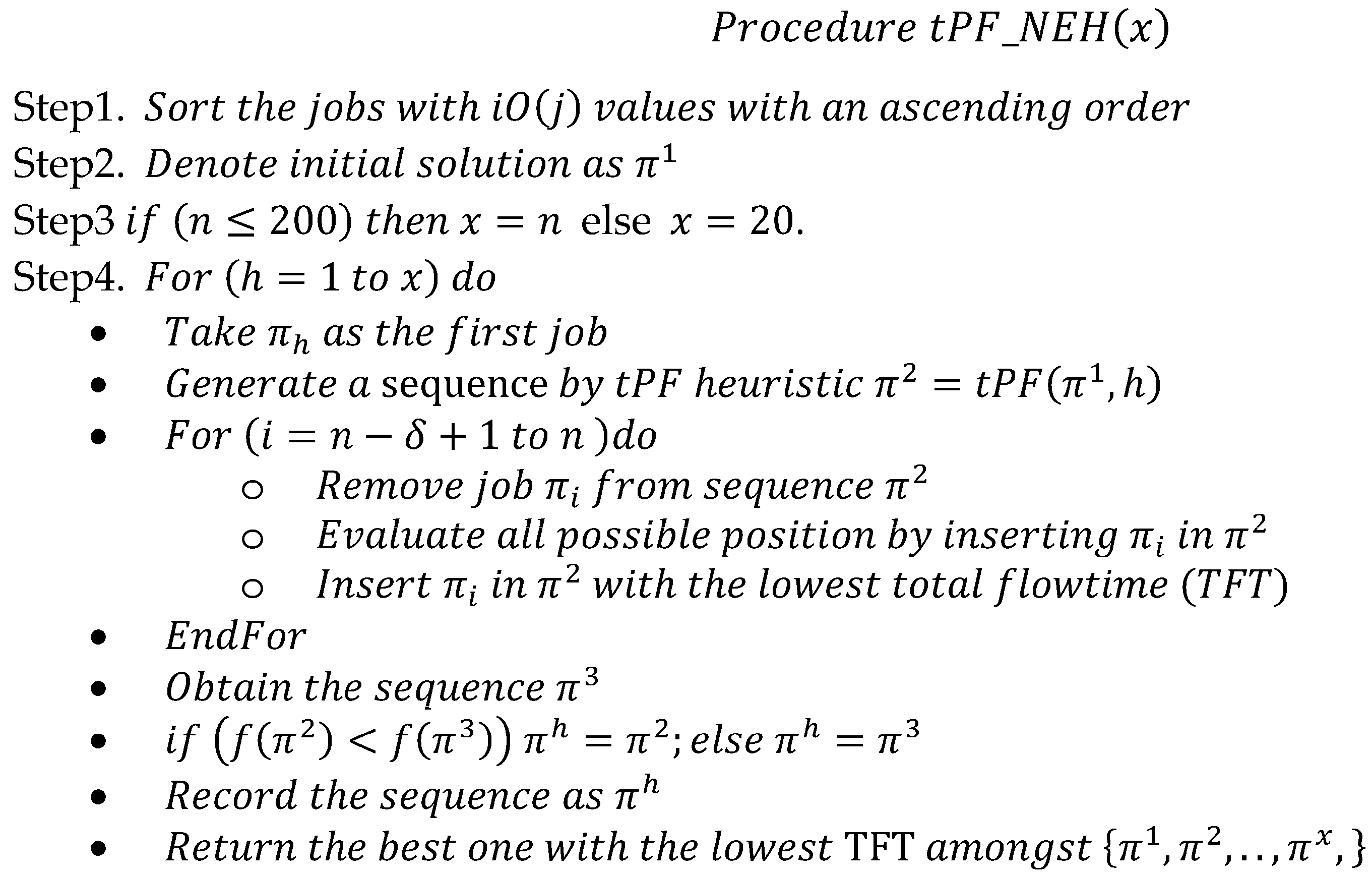
3.1. Initial Solution
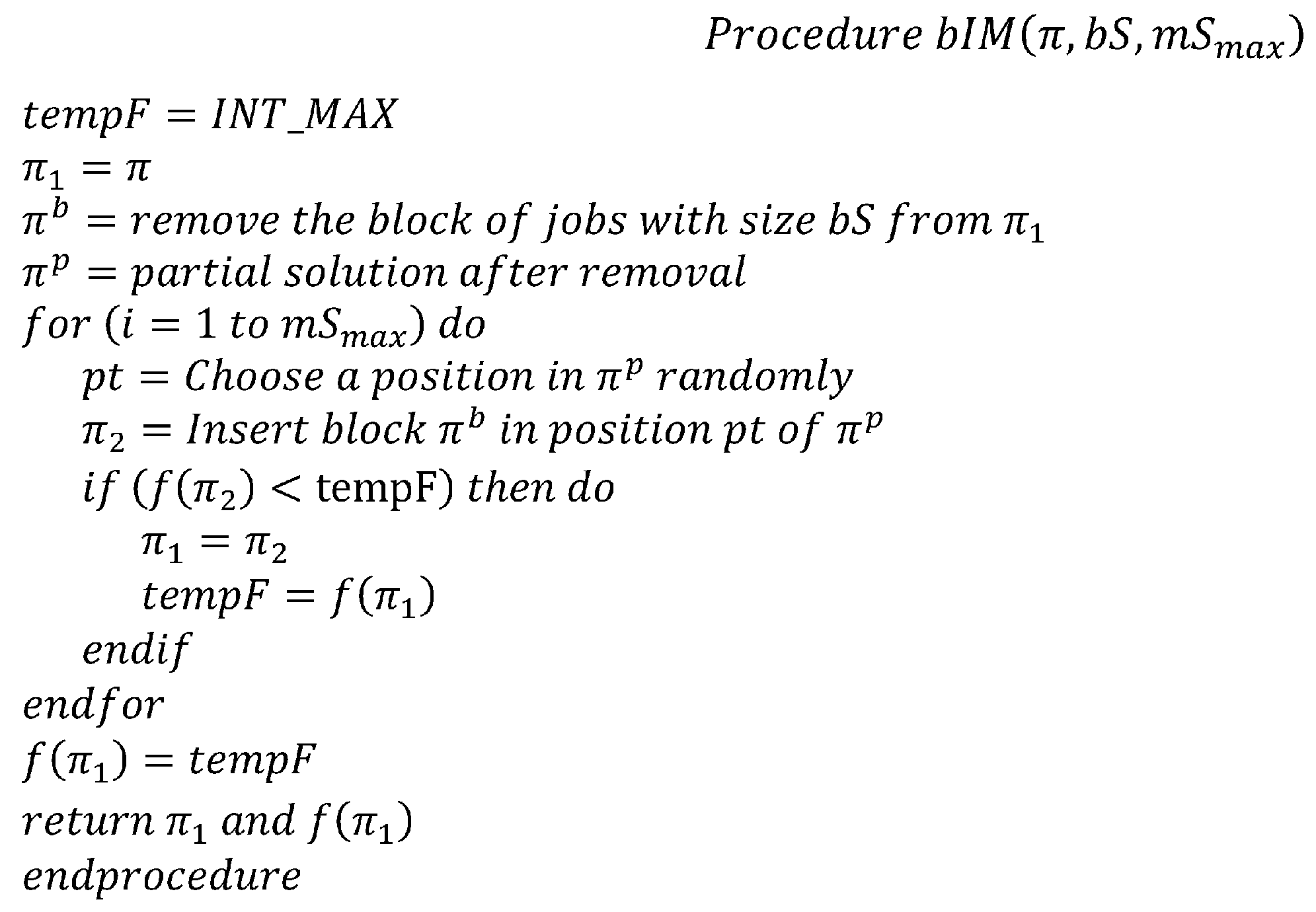
3.2. Block Insertion Move Procedure
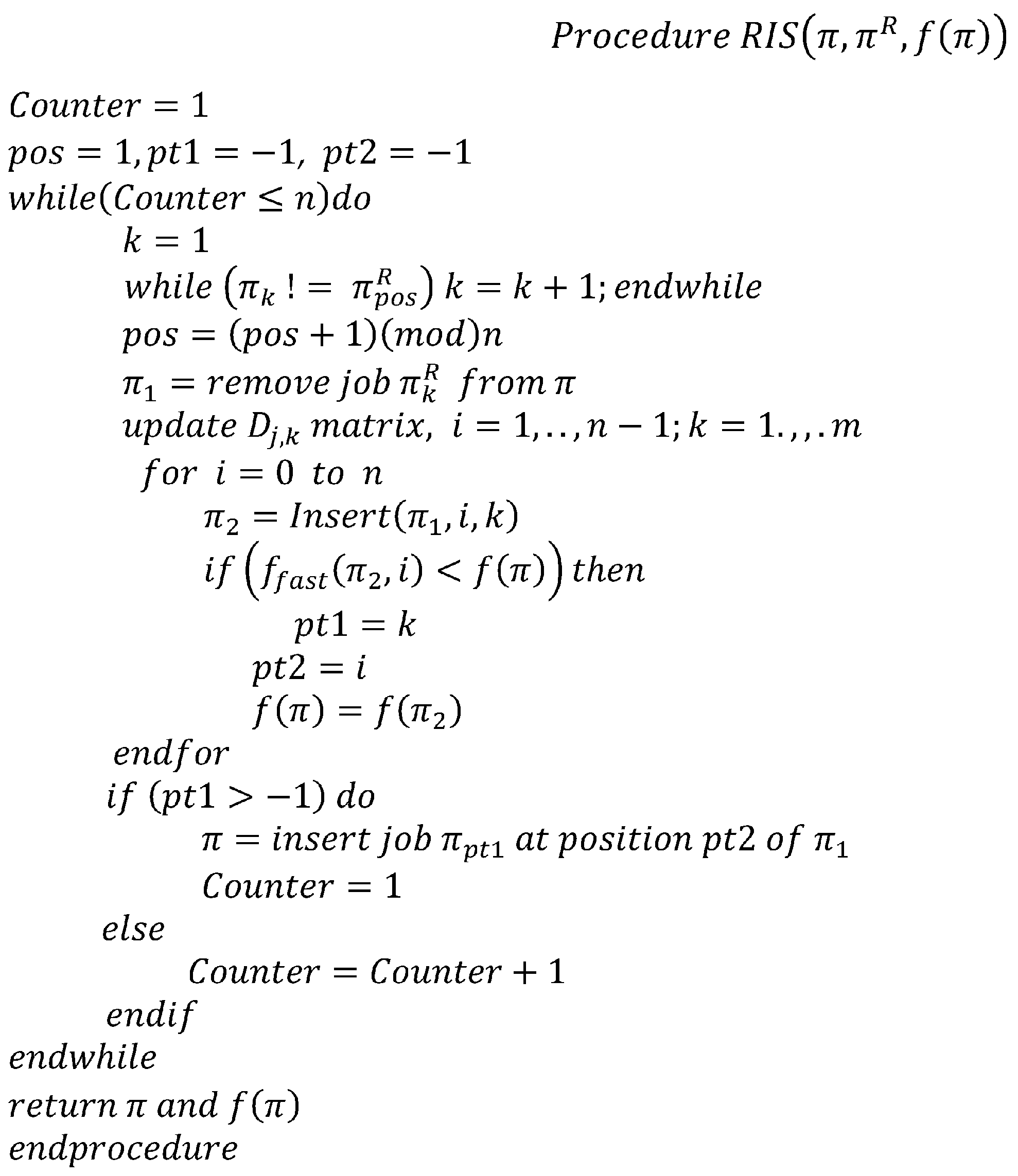
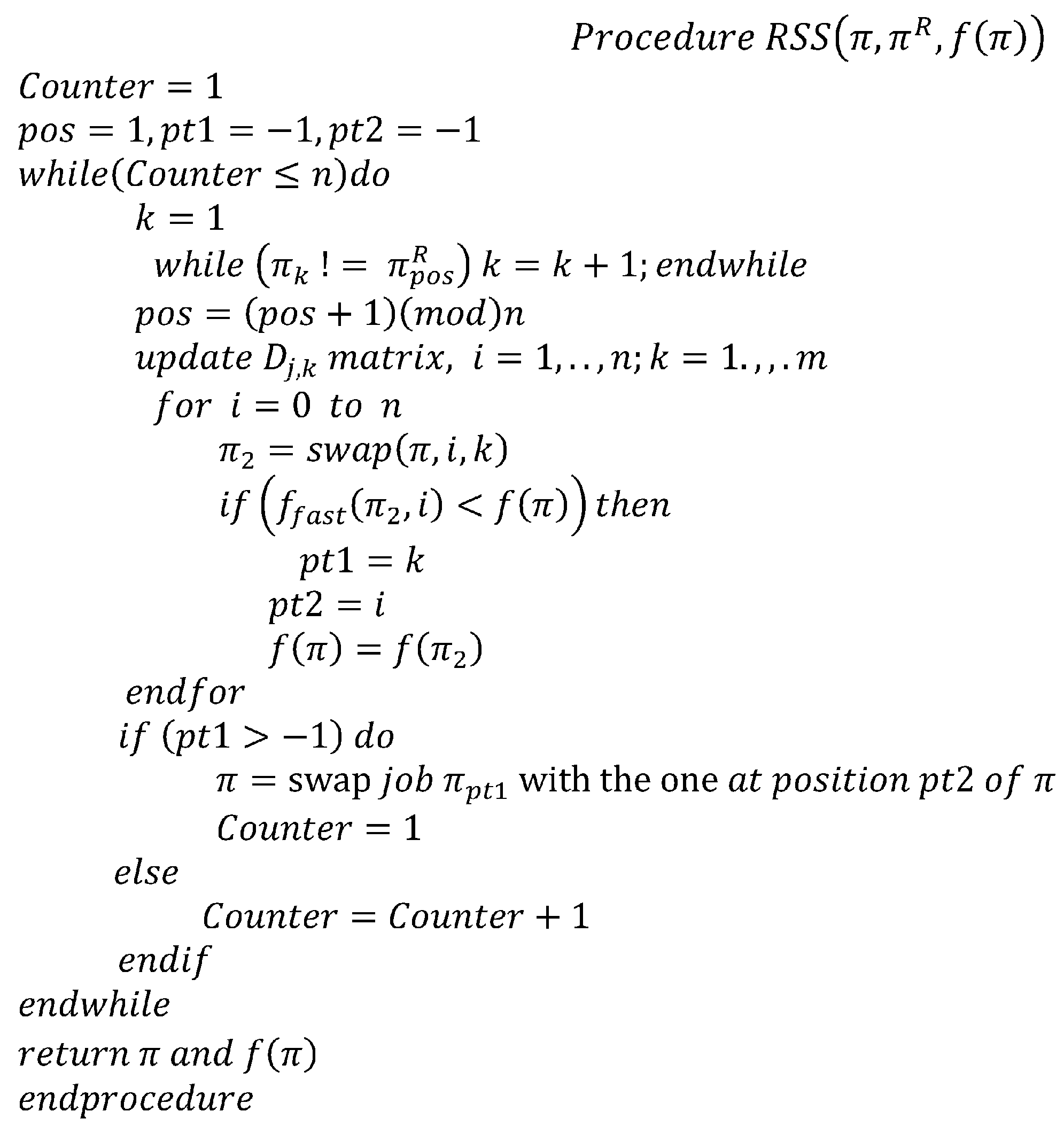
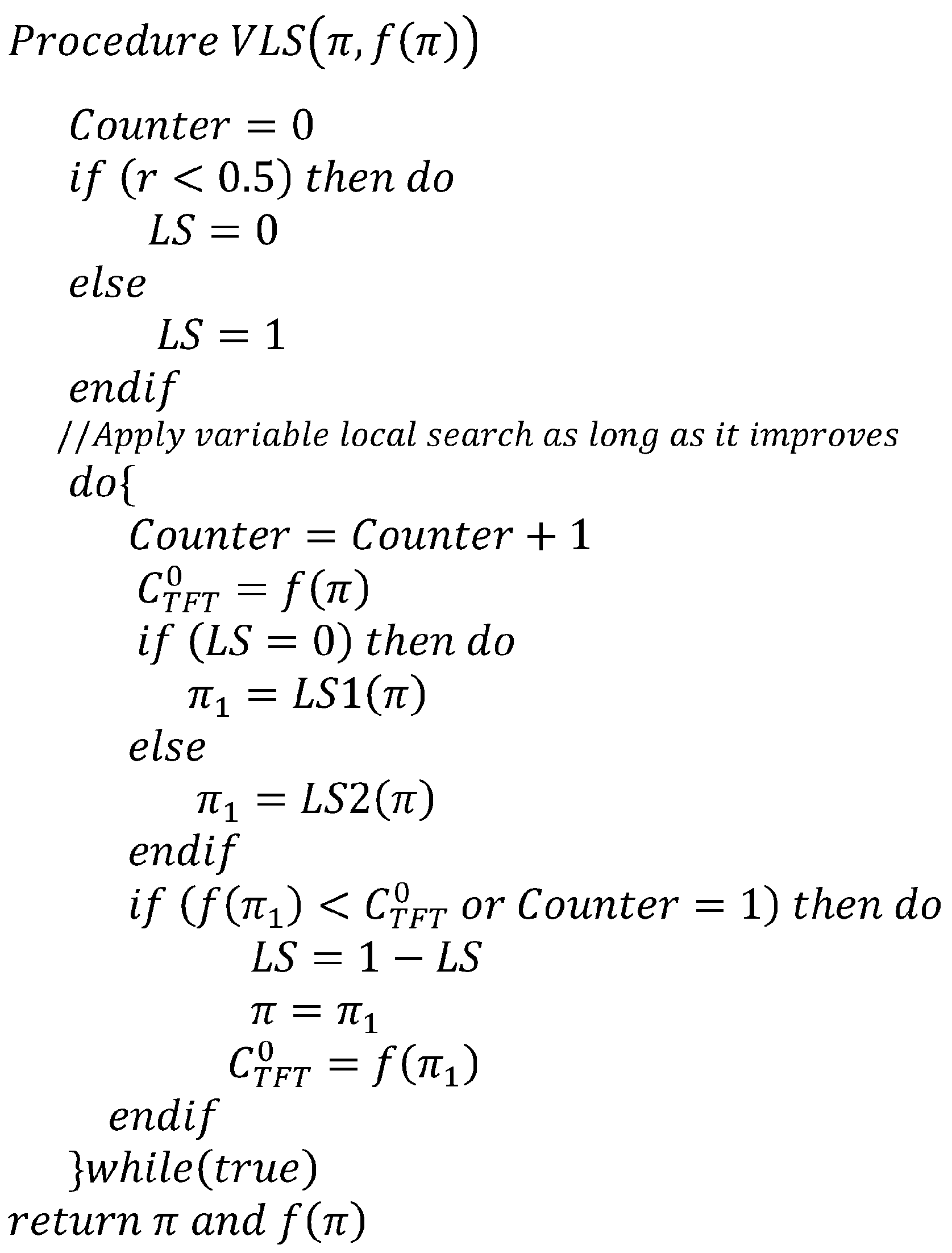
3.3. Variable Local Search
4. Parameter Tuning
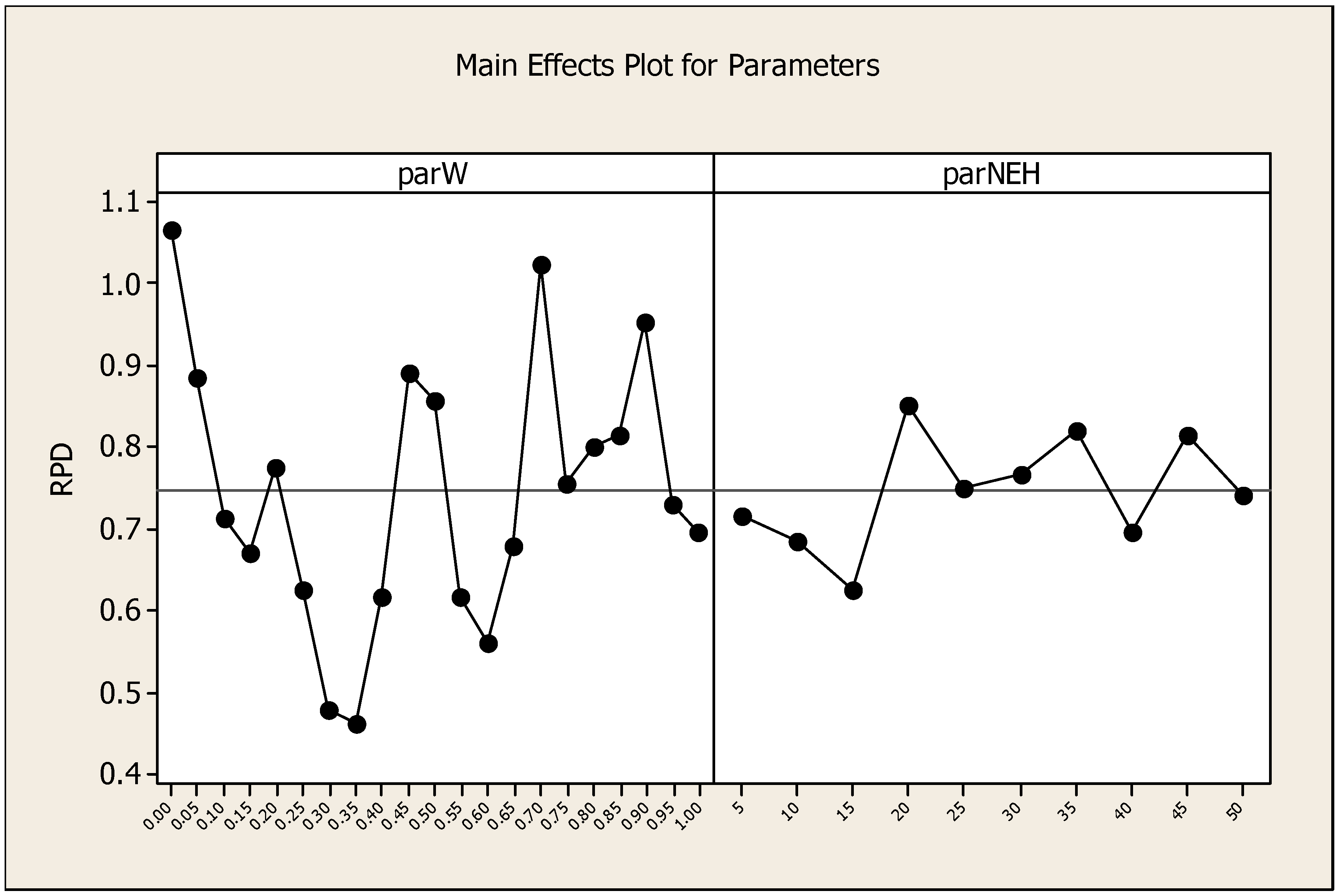
4.1. Parameter Tuning of PFT_NEX(x) Heuristic
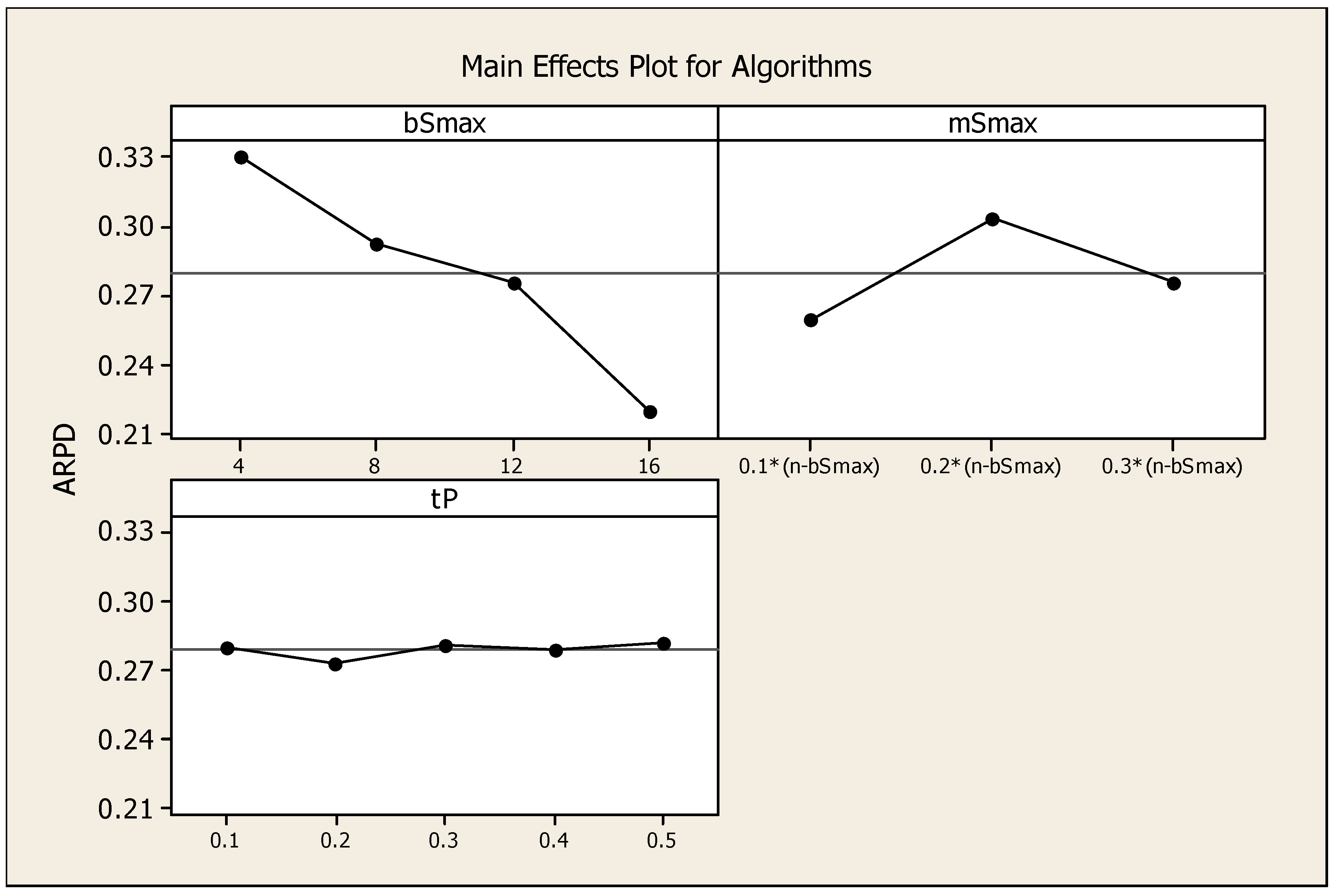
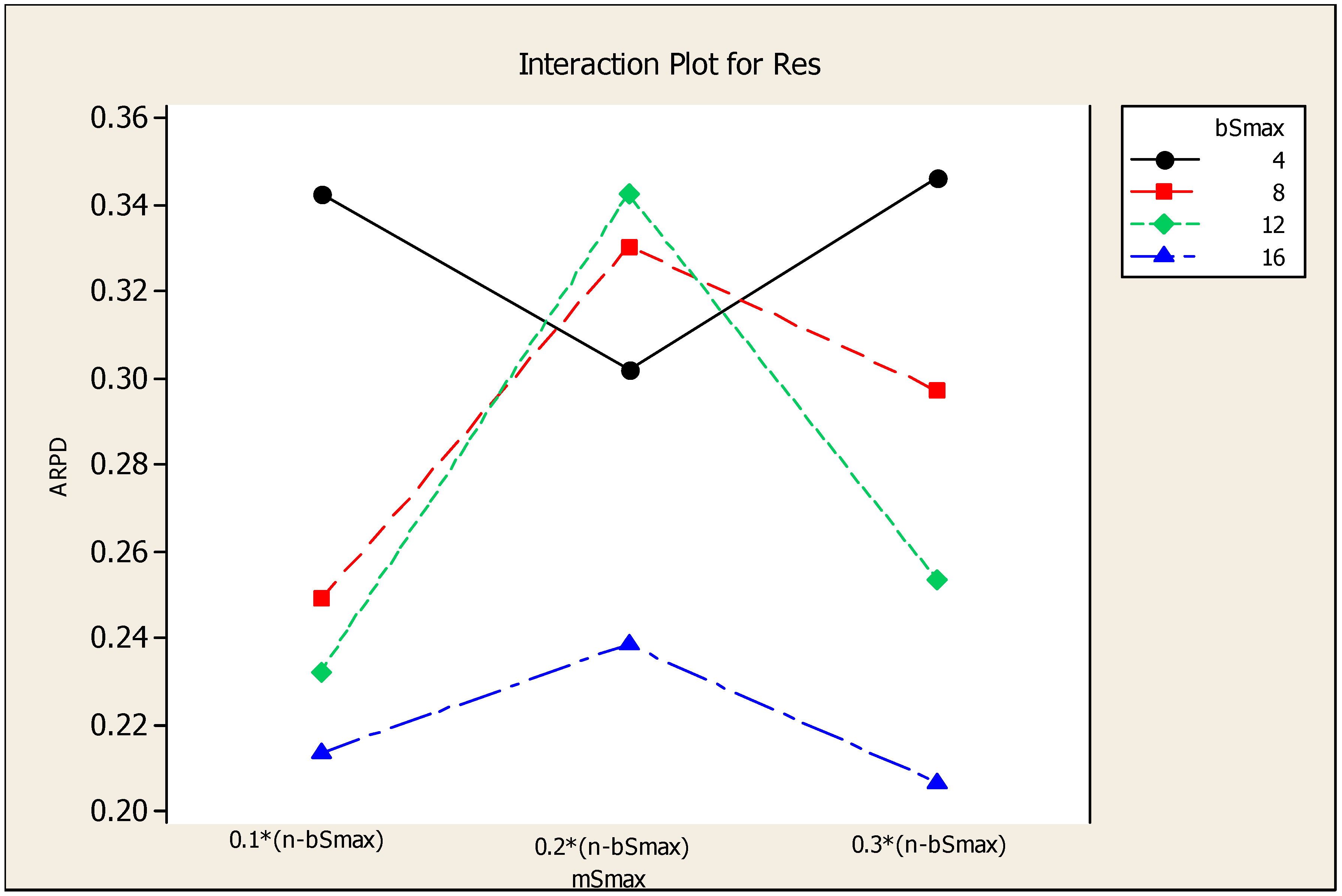
4.2. Parameter Tuning of VBIH Algorithm
5. Computational Results
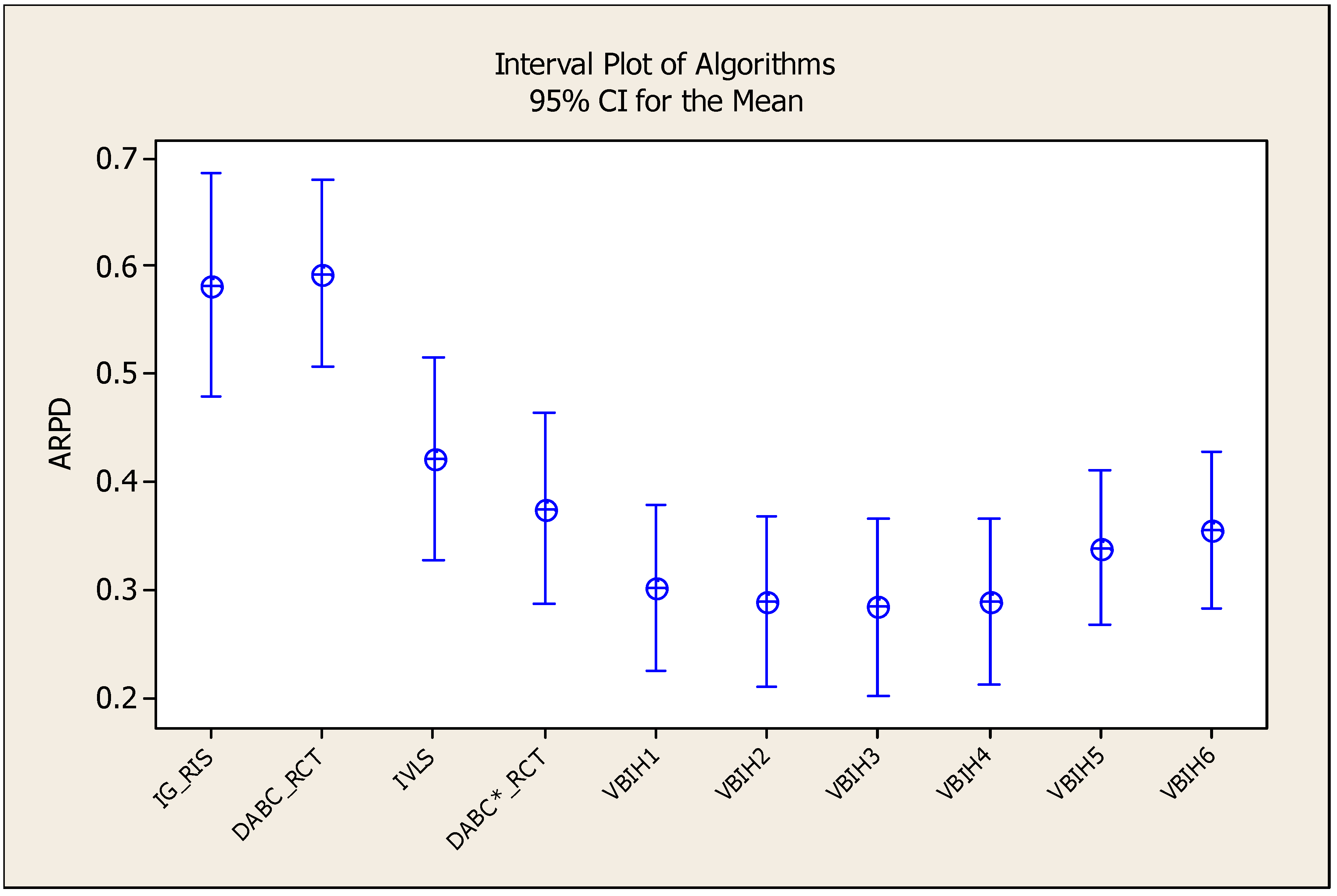
- DABC_RCT in [41]. The DABC_RCT algorithm is a very efficient algorithm and has three phases. In the employed bee phase, the TNO procedure is employed with the VLS local search. In the onlooker bee phase, the path-relinking approach is employed to generate the onlooker bees. In the scout bee phase, HPF2 is used to generate the scout bees. We refer to [41] for the details. We have coded the DABC_RCT algorithm in Visual C+13 to have a fair comparison. Note that the DABC_RCT algorithm uses HPF2 heuristic as an initial solution. Since our PFT_NEH(x) heuristic is substantially better than HPF2 heuristic, we employ the PFT_NEH(x) heuristic with and as one of the solution in the population. The rest of the population individuals are constructed randomly as suggested in the DABC_RCT algorithm and we denote it as the DABC*_RCT algorithm to have a fair comparison. The same parameters are also used which are suggested in the DABC_RCT algorithm [41]. Note that fast fitness calculation is employed to accelerate the insertion and swap neighborhood structures in the VLS local search they employed in the TNO procedure.
- IG_RIS algorithm in [47,54,55,56,57,58,59]. To be fair again, we employ PFT_NEH(x) heuristic with and as an initial solution in the IG_RIS algorithm. IG_RIS algorithm relies on the destruction and construction procedure, where number of jobs is removed from a solution and they are reinserted to the partial solution sequentially. Then RIS local search is applied to the solution obtained after destruction and construction procedure. Note that fast fitness calculation is employed to accelerate the RIS insertion local search as in this paper. It is also employed in the destruction and construction procedure, too.
- VBIH algorithms in this paper. Since the PFT_NEH(x) heuristics provide very diversified initial solutions, we run the VBIH algorithm with values with 0.25, 0.30, 0.35, 0.40, 0.55 and 0.60 with . Then we denote them as VBIH1, VBIH2, VBIH3, VBIH4, VBIH5 and VBIH6. In addition, when the maximum block size is equal to 1, the VBIH algorithm becomes an iterated local search. In other words, the current solution is perturbed with several insertion moves and then the VLS local search is applied to the solution after perturbation. Then, the acceptance criterion is imposed to the solution obtained. We denote this variant of the VBIH algorithm as IVLS algorithm.
6. Conclusions
Supplementary Materials
Author Contributions
Conflicts of Interest
References
- Błażewicz, J.; Ecker, K.H.; Pesch, E.; Schmidt, G.; Weglarz, J. Handbook on Scheduling: From Theory to Applications; Springer: Berlin/Heidelberg, Germany, 2007. [Google Scholar]
- Pan, Q.K.; Ruiz, R. An estimation of distribution algorithm for lot-streaming flow shop problems with setup times. Omega 2012, 40, 166–180. [Google Scholar] [CrossRef]
- Vallada, E.; Ruiz, R. Genetic algorithms with path relinking for the minimum tardiness permutation flowshop problem. Omega 2010, 38, 57–67. [Google Scholar] [CrossRef]
- Ruiz-Torres, A.J.; Ho, T.J.; Ablanedo-Rosas, J.H. Makespan and workstation utilization minimization in a flowshop with operations flexibility. Omega 2011, 39, 273–282. [Google Scholar] [CrossRef]
- Grabowski, J.; Pempera, J. Sequencing of jobs in some production system. Eur. J. Oper. Res. 2000, 125, 535–550. [Google Scholar] [CrossRef]
- Ronconi, D.P. A note on constructive heuristics for the flowshop problem with blocking. Int. J. Prod. Econ. 2004, 87, 39–48. [Google Scholar] [CrossRef]
- Hall, N.G.; Sriskandarajah, C. A survey of machine scheduling problems with blocking and no-wait in process. Oper. Res. 1996, 44, 510–525. [Google Scholar] [CrossRef]
- Graham, R.L.; Lawler, E.L.; Lenstra, J.K.; Rinnooy Kan, A.H.G. Optimization and approximation in deterministic sequencing and scheduling: A survey. Ann. Discret. Math. 1979, 5, 287–362. [Google Scholar]
- Gilmore, P.C.; Lawler, E.L.; Shmoys, D.B. Well-solved special cases. In The Traveling Salesman Problem: A Guided Tour of Combinatorial Optimization; Lawler, E.L., Lenstra, K.L., Rinooy Kan, A.H.G., Shmoys, D.B., Eds.; John Wiley & Sons: Hoboken, NJ, USA, 1985; pp. 87–143. [Google Scholar]
- McCormick, S.T.; Pinedo, M.L.; Shenker, S.; Wolf, B. Sequencing in an assembly line with blocking to minimize cycle time. Oper. Res. 1989, 37, 925–936. [Google Scholar] [CrossRef]
- Leisten, R. Flowshop sequencing problems with limited buffer storage. Int. J. Prod. Res. 1990, 28, 2085–2100. [Google Scholar] [CrossRef]
- Nawaz, M.; Enscore, E.E.J.; Ham, I. A heuristic algorithm for the m-machine, n-job flow shop sequencing problem. Omega 1983, 11, 91–95. [Google Scholar] [CrossRef]
- Ronconi, D.P.; Armentano, V.A. Lower bounding schemes for flowshops with blocking in-process. J. Oper. Res. Soc. 2001, 52, 1289–1297. [Google Scholar] [CrossRef]
- Abadi, I.N.K.; Hall, N.G.; Sriskandarajh, C. Minimizing cycle time in a blocking flowshop. Oper. Res. 2000, 48, 177–180. [Google Scholar] [CrossRef]
- Ronconi, D.P.; Henriques, L.R.S. Some heuristic algorithms for total tardiness minimization in a flowshop with blocking. Omega 2009, 37, 272–281. [Google Scholar] [CrossRef]
- Pan, Q.K.; Wang, L. Effective heuristics for the blocking flowshop scheduling problem with makespan minimization. Omega 2012, 40, 218–229. [Google Scholar] [CrossRef]
- Liu, J.Y.; Reeves, C.R. Constructive and composite heuristic solutions to the P// ∑ Ci scheduling problem. Eur. J. Oper. Res. 2001, 132, 439–452. [Google Scholar] [CrossRef]
- Caraffa, V.; Ianes, S.; Bagchi, T.P.; Sriskandarajah, C. Minimizing makespan in a blocking flowshop using genetic algorithms. Int. J. Prod. Econ. 2001, 70, 101–115. [Google Scholar] [CrossRef]
- Ronconi, D.P. A branch-and-bound algorithm to minimize the makespan in a flowshop problem with blocking. Ann. Oper. Res. 2005, 138, 53–65. [Google Scholar] [CrossRef]
- Taillard, E. Benchmarks for basic scheduling problems. Eur. J. Oper. Res. 1993, 64, 278–285. [Google Scholar] [CrossRef]
- Grabowski, J.; Pempera, J. The permutation flow shop problem with blocking. A tabu search approach. Omega 2007, 35, 302–311. [Google Scholar] [CrossRef]
- Wang, L.; Zhang, L.; Zheng, D. An effective hybrid genetic algorithm for flow shop scheduling with limited buffers. Comput. Oper. Res. 2006, 33, 2960–2971. [Google Scholar] [CrossRef]
- Liu, B.; Wang, L.; Jin, Y. An effective hybrid PSO-based algorithm for flow shop scheduling with limited buffers. Comput. Oper. Res. 2008, 35, 2791–2806. [Google Scholar] [CrossRef]
- Qian, B.; Wang, L.; Huang, D.X.; Wang, X. An effective hybrid DE-based algorithm for flow shop scheduling with limited buffers. Int. J. Prod. Res. 2009, 47, 1–24. [Google Scholar] [CrossRef]
- Liang, J.J.; Pan, Q.; Tiejun, C.; Wang, L. Solving the blocking flow shop scheduling problem by a dynamic multi-swarm particle swarm optimizer. Int. J. Adv. Manuf. Technol. 2011, 55, 755–762. [Google Scholar] [CrossRef]
- Wang, L.; Pan, Q.K.; Tasgetiren, M.F. A Hybrid Harmony Search Algorithm for the Blocking Permutation Flow Shop Scheduling Problem. Comput. Ind. Eng. 2011, 61, 76–83. [Google Scholar] [CrossRef]
- Wang, L.; Pan, Q.K.; Suganthan, P.N.; Wang, W.H.; Wang, Y.M. A novel hybrid discrete differential evolution algorithm for blocking flow shop scheduling problems. Comput. Oper. Res. 2010, 37, 509–520. [Google Scholar] [CrossRef]
- Ribas, I.; Companys, R.; Tort-Martorell, X. An iterated greedy algorithm for the flowshop scheduling with blocking. Omega 2011, 39, 293–301. [Google Scholar] [CrossRef]
- Wang, C.; Song, S.; Gupta, J.N.D.; Wu, C. A three-phase algorithm for flowshop scheduling with blocking to minimize makespan. Comput. Oper. Res. 2012, 39, 2880–2887. [Google Scholar] [CrossRef]
- Lin, S.W.; Ying, K.C. Minimizing makespan in a blocking flowshop using a revised artificial immune system algorithm. Omega 2013, 41, 383–389. [Google Scholar] [CrossRef]
- Pan, Q.K.; Wang, L.; Sang, H.Y.; Li, J.Q.; Liu, M. A high performing memetic algorithm for the flowshop scheduling problem with blocking. IEEE Trans. Autom. Sci. Eng. 2013, 10, 741–756. [Google Scholar]
- Ribas, I.; Companys, R.; Tort-Martorell, X. A competitive variable neighbourhood search algorithm for the blocking flow shop problem. Eur. J. Ind. Eng. 2013, 7, 729–754. [Google Scholar] [CrossRef]
- Ding, J.-Y.; Song, S.; Gupta, N.D.J.; Wang, C.; Zhang, R.; Wu, C. New block properties for flowshop scheduling with blocking and their application in an iterated greedy algorithm. Int. J. Prod. Res. 2015, 54, 4759–4772. [Google Scholar] [CrossRef]
- Armentano, V.A.; Ronconi, D.P. Minimização do tempo total de atraso no problema de flowshop com buffer zero através de busca tabu. Gestao Produçao 2000, 7, 352–362. (In Portuguese) [Google Scholar] [CrossRef]
- Ribas, I.; Companys, R.; Tort-Martorell, X. An efficient iterated local search algorithm for the total tardiness blocking flow shop problem. Int. J. Prod. Res. 2013, 51, 5238–5252. [Google Scholar] [CrossRef]
- Wang, L.; Pan, Q.K.; Tasgetiren, M.F. Minimizing the total flow time in a flow shop with blocking by using hybrid harmony search algorithms. Expert Syst. Appl. 2010, 37, 7929–7936. [Google Scholar] [CrossRef]
- Deng, G.; Xu, Z.; Gu, X. A discrete artificial bee colony algorithm for minimizing the total flow time in the blocking flow shop scheduling. Chin. J. Chem. Eng. 2012, 20, 1067–1073. [Google Scholar] [CrossRef]
- Khorasanian, D.; Moslehi, G. An iterated greedy algorithm for solving the blocking flowshop scheduling problem with total flow time criteria. Int. J. Ind. Eng. Prod. Res. 2012, 23, 301–308. [Google Scholar]
- Moslehi, G.; Khorasanian, D. Optimizing blocking flow shop scheduling total completion time criterion. Comput. Oper. Res. 2013, 40, 1874–1883. [Google Scholar] [CrossRef]
- Ribas, I.; Companys, R. Efficient heuristic algorithms for the blocking flow shop scheduling problem with total flow time minimization. Comput. Ind. Eng. 2015, 87, 30–39. [Google Scholar] [CrossRef]
- Ribas, I.; Companys, R. Xavier Tort-Martorell, An efficient Discrete Artificial Bee Colony algorithm for the blocking flow shop problem with total flowtime minimization. Expert Syst. Appl. 2015, 42, 6155–6167. [Google Scholar] [CrossRef] [Green Version]
- Lia, X.; Wang, Q.; Wu, C. Efficient composite heuristics for total flowtime minimization in permutation flowshops. Omega 2009, 37, 155–164. [Google Scholar] [CrossRef]
- Kirlik, G.; Oguz, C. A Variable Neighborhood Search for Minimizing Total Weighted Tardiness with Sequence Dependent Setup Times on a Single Machine. Comput. Oper. Res. 2012, 39, 1506–1520. [Google Scholar] [CrossRef]
- Subramanian, A.; Battarra, M.; Potts, C.N. An Iterated Local Search heuristic for the single machine total weighted tardiness scheduling problem with sequence-dependent setup times. Int. J. Prod. Res. 2014, 52, 2729–2742. [Google Scholar] [CrossRef]
- Xu, H.; Lü, Z.; Cheng, T.C.E. Iterated Local Search for single-machine scheduling with sequence dependent setup times to minimize total weighted tardiness. J. Sched. 2014, 17, 271–287. [Google Scholar] [CrossRef]
- González, M.A.; Vela, C.R. An efficient memetic algorithm for total weighted tardiness minimization in a single machine with setups. Appl. Soft Comput. 2015, 37, 506–518. [Google Scholar] [CrossRef]
- Tasgetiren, M.F.; Kizilay, D.; Pan, Q.K.; Suganthan, P.N. Iterated Greedy Algorithms for the Blocking Flowshop Scheduling Problem with Makespan Criterion. Comput. Oper. Res. 2016. [Google Scholar] [CrossRef]
- Mladenovic, N.; Hansen, P. Variable neighborhood search. Comput. Oper. Res. 1997, 24, 1097–1100. [Google Scholar] [CrossRef]
- Tasgetiren, M.F.; Liang, Y.-C.; Sevkli, M.; Gencyilmaz, G. A particle swarm optimization algorithm for makespan and total flowtime minimization in the permutation flowshop sequencing problem. Eur. J. Oper. Res. 2007, 177, 1930–1947. [Google Scholar] [CrossRef]
- Pan, Q.-K.; Tasgetiren, M.F.; Liang, Y.-C. A Discrete Particle Swarm Optimization Algorithm for the No-Wait Flowshop Scheduling Problem with Makespan and Total Flowtime Criteria. Comput. Oper. Res. 2008, 35, 2807–2839. [Google Scholar] [CrossRef]
- Pan, Q.-K.; Wang, L.; Tasgetiren, M.F.; Zhao, B.-H. A hybrid discrete particle swarm optimization algorithm for the no-wait flow shop scheduling problem with makespan criterion. Int. J. Adv. Manuf. Technol. 2008, 38, 337–347. [Google Scholar] [CrossRef]
- Tasgetiren, M.F.; Liang, Y.-C.; Sevkli, M.; Gencyilmaz, G. Particle swarm optimization and differential evolution for single machine total weighted tardiness problem. Int. J. Prod. Res. 2006, 44, 4737–4754. [Google Scholar] [CrossRef]
- Tasgetiren, M.F.; Sevkli, M.; Liang, Y.-C.; Yenisey, M.M. A particle swarm optimization and differential evolution algorithms for job shop scheduling problem. Int. J. Oper. Res. 2006, 3, 120–135. [Google Scholar]
- Tasgetiren, M.F.; Pan, Q.K.; Suganthan, P.N.; Buyukdagli, O. A variable iterated greedy algorithm with differential evolution for the no-idle permutation flowshop scheduling problem. Comput. Oper. Res. 2013, 40, 1729–1743. [Google Scholar] [CrossRef]
- Pan, Q.K.; Tasgetiren, M.F.; Liang, Y.C. A discrete differential evolution algorithm for the permutation flowshop scheduling problem. Comput. Ind. Eng. 2008, 55, 795–816. [Google Scholar] [CrossRef]
- Tasgetiren, M.F.; Pan, Q.K.; Liang, Y.C. A discrete differential evolution algorithm for the single machine total weighted tardiness problem with sequence dependent setup times. Comput. Oper. Res. 2009, 36, 1900–1915. [Google Scholar] [CrossRef]
- Tasgetiren, M.F.; Pan, Q.K.; Suganthan, P.N.; Chen, A.H.L. A discrete artificial bee colony algorithm for the total flowtime minimization in permutation flow shops. Inf. Sci. 2011, 181, 3459–3475. [Google Scholar] [CrossRef]
- Tasgetiren, M.F.; Pan, Q.K.; Suganthan, P.N.; Oner, A. A Discrete Artificial Bee Colony Algorithm for the No-Idle Permutation Flowshop Scheduling Problem with the Total Tardiness Criterion. Appl. Math. Model. 2013, 37, 6758–6779. [Google Scholar] [CrossRef]
- Tasgetiren, M.F.; Pan, Q.K.; Suganthan, P.N.; Chua, T.J. A Differential Evolution Algorithm for the No-Idle Flowshop Scheduling Problem with Total Tardiness Criterion. Int. J. Prod. Res. 2011, 49, 5033–5050. [Google Scholar] [CrossRef]
- Osman, I.; Potts, C. Simulated annealing for permutation flow-shop scheduling. Omega 1989, 17, 551–557. [Google Scholar] [CrossRef]
- Montgomery, D.C. Design and Analysis of Experiments; John Wiley & Sons: Hoboken, NJ, USA, 2008. [Google Scholar]
- Pan, Q.K.; Ruiz, R. Local search methods for the flowshop scheduling problem with flowtime minimization. Eur. J. Oper. Res. 2012, 222, 31–43. [Google Scholar] [CrossRef]
- Schenker, N.; Gentleman, J.F. On judging the significance of differences by examining the overlap between confidence intervals. Am. Stat. 2001, 55, 182–186. [Google Scholar] [CrossRef]


| Values and CPU (s) | |||||||||||||||
|---|---|---|---|---|---|---|---|---|---|---|---|---|---|---|---|
| n × m | HPF2 [41] | NHPF1 [40] | NHPF2 [40] | CPU (s) | CPU (s) | CPU (s) | CPU (s) | CPU (s) | CPU (s) | ||||||
| 20 × 5 | 4.038 | 2.928 | 3.059 | 1.368 | 0.002 | 1.190 | 0.000 | 1.158 | 0.003 | 1.014 | 0.003 | 1.264 | 0.000 | 1.190 | 0.002 |
| 20 × 10 | 3.156 | 2.719 | 2.340 | 1.069 | 0.000 | 1.228 | 0.003 | 1.005 | 0.002 | 1.154 | 0.000 | 1.175 | 0.000 | 1.005 | 0.003 |
| 20 × 20 | 3.989 | 2.857 | 2.766 | 1.011 | 0.002 | 0.942 | 0.003 | 1.016 | 0.003 | 1.063 | 0.003 | 1.009 | 0.002 | 1.047 | 0.003 |
| 50 × 5 | 3.929 | 3.903 | 3.528 | 3.029 | 0.022 | 2.775 | 0.023 | 2.774 | 0.024 | 3.204 | 0.025 | 2.881 | 0.022 | 2.915 | 0.025 |
| 50 × 10 | 3.664 | 4.191 | 3.665 | 2.718 | 0.039 | 2.651 | 0.039 | 2.608 | 0.041 | 2.671 | 0.039 | 2.655 | 0.041 | 2.871 | 0.041 |
| 50 × 20 | 5.318 | 4.398 | 4.237 | 2.453 | 0.078 | 2.409 | 0.077 | 2.274 | 0.073 | 2.310 | 0.075 | 2.210 | 0.080 | 2.258 | 0.078 |
| 100 × 5 | 3.816 | 3.757 | 3.668 | 2.989 | 0.116 | 2.743 | 0.114 | 2.702 | 0.125 | 2.692 | 0.116 | 2.822 | 0.116 | 2.913 | 0.120 |
| 100 × 10 | 4.087 | 4.450 | 3.964 | 2.611 | 0.211 | 2.783 | 0.216 | 2.598 | 0.213 | 2.569 | 0.213 | 2.755 | 0.223 | 2.863 | 0.217 |
| 100 × 20 | 5.554 | 4.428 | 4.539 | 2.223 | 0.431 | 2.030 | 0.434 | 2.125 | 0.433 | 2.064 | 0.433 | 2.353 | 0.434 | 2.207 | 0.436 |
| 200 × 10 | 2.362 | 2.505 | 1.915 | 1.057 | 1.730 | 0.944 | 1.740 | 1.053 | 1.737 | 1.070 | 1.736 | 1.160 | 1.731 | 1.336 | 1.736 |
| 200 × 20 | 2.811 | 2.676 | 2.478 | 0.777 | 3.553 | 0.669 | 3.580 | 0.889 | 3.594 | 0.780 | 3.552 | 1.000 | 3.552 | 1.122 | 3.555 |
| 500 × 20 | 1.595 | 1.464 | 1.533 | −0.177 | 2.352 | −0.158 | 2.402 | −0.111 | 2.358 | −0.082 | 2.349 | 0.066 | 2.350 | 0.048 | 2.352 |
| 200 × 5 | 2.394 | 2.260 | 1.936 | 1.400 | 0.917 | 1.292 | 0.920 | 1.264 | 0.917 | 1.314 | 0.919 | 1.727 | 0.917 | 1.833 | 0.920 |
| 500 × 5 | 1.191 | 1.330 | 1.027 | 0.545 | 0.755 | 0.356 | 0.758 | 0.317 | 0.750 | 0.475 | 0.775 | 0.825 | 0.761 | 0.916 | 0.758 |
| 500 × 10 | 1.398 | 1.399 | 1.307 | 0.272 | 1.194 | 0.247 | 1.195 | 0.353 | 1.189 | 0.248 | 1.188 | 0.477 | 1.191 | 0.564 | 1.191 |
| Average | 3.287 | 3.018 | 2.797 | 1.556 | 0.760 | 1.473 | 0.767 | 1.468 | 0.764 | 1.503 | 0.762 | 1.625 | 0.761 | 1.673 | 0.762 |
| 3 | 0.095370 | 0.095370 | 0.031790 | 98.55 | 0.00 | |
| 2 | 0.019873 | 0.019873 | 0.009937 | 30.80 | 0.00 | |
| 4 | 0.000676 | 0.000676 | 0.000169 | 0.52 | 0.72 | |
| 6 | 0.039930 | 0.039930 | 0.006655 | 20.63 | 0.00 | |
| 12 | 0.002395 | 0.002395 | 0.000200 | 0.62 | 0.81 | |
| 8 | 0.001585 | 0.001585 | 0.000198 | 0.61 | 0.76 | |
| 24 | 0.007742 | 0.007742 | 0.000323 | - | - | |
| 59 | 0.167569 | - | - | - | - |
| n × m | IG_RIS | DABC_RCT | IVLS | DABC*_RCT | VBIH1 | VBIH2 | VBIH3 | VBIH4 | VBIH5 | VBIH6 |
|---|---|---|---|---|---|---|---|---|---|---|
| 20 × 5 | 0.049 | 0.004 | 0.068 | 0.006 | 0.001 | 0.000 | 0.000 | 0.000 | 0.000 | 0.000 |
| 20 × 10 | 0.016 | 0.021 | 0.151 | 0.031 | 0.000 | 0.000 | 0.000 | 0.000 | 0.000 | 0.000 |
| 20 × 20 | 0.010 | 0.015 | 0.032 | 0.002 | 0.000 | 0.000 | 0.000 | 0.000 | 0.000 | 0.000 |
| 50 × 5 | 0.901 | 0.788 | 0.713 | 0.490 | 0.418 | 0.354 | 0.346 | 0.376 | 0.296 | 0.325 |
| 50 × 10 | 0.819 | 0.752 | 0.916 | 0.752 | 0.562 | 0.455 | 0.457 | 0.424 | 0.463 | 0.502 |
| 50 × 20 | 0.521 | 0.561 | 0.652 | 0.490 | 0.318 | 0.378 | 0.316 | 0.355 | 0.330 | 0.321 |
| 100 × 5 | 1.555 | 1.135 | 1.133 | 0.937 | 0.650 | 0.764 | 0.709 | 0.650 | 0.696 | 0.714 |
| 100 × 10 | 1.639 | 1.301 | 1.358 | 1.285 | 1.070 | 1.179 | 1.126 | 1.098 | 1.112 | 1.118 |
| 100 × 20 | 1.147 | 1.279 | 0.927 | 0.983 | 0.759 | 0.833 | 0.799 | 0.903 | 0.796 | 0.750 |
| 200 × 10 | 0.633 | 0.559 | 0.236 | 0.312 | 0.427 | 0.243 | 0.377 | 0.293 | 0.297 | 0.308 |
| 200 × 20 | 0.337 | 0.581 | 0.193 | 0.201 | 0.146 | 0.227 | 0.211 | 0.255 | 0.430 | 0.421 |
| 500 × 20 | −0.229 | 0.426 | −0.381 | −0.274 | −0.353 | −0.374 | −0.395 | −0.303 | −0.192 | −0.185 |
| 200 × 5 | 0.854 | 0.470 | 0.373 | 0.358 | 0.392 | 0.325 | 0.341 | 0.372 | 0.388 | 0.401 |
| 500 × 5 | 0.259 | 0.397 | −0.014 | −0.022 | 0.150 | −0.012 | −0.053 | −0.042 | 0.299 | 0.369 |
| 500 × 10 | 0.234 | 0.607 | −0.033 | 0.092 | 0.000 | −0.031 | 0.035 | −0.046 | 0.174 | 0.282 |
| Average | 0.583 | 0.593 | 0.422 | 0.376 | 0.303 | 0.289 | 0.285 | 0.289 | 0.339 | 0.355 |
| Algorithm vs. algorithm | 95% CI for Mean Difference | p-Value |
|---|---|---|
| IVLS − DABC*_RCT | (0.0041, 0.0875) | 0.032 |
| VBIH1 − DABC*_RCT | (−0.1162, −0.0298) | 0.001 |
| VBIH2 − DABC*_RCT | (−0.1242, −0.0486) | 0.000 |
| VBIH3 − DABC*_RCT | (−0.1193, −0.0639) | 0.000 |
| VBIH4 − DABC*_RCT | (−0.1258, −0.0474) | 0.000 |
| VBIH5 − DABC*_RCT | (−0.0843, 0.0117) | 0.137 |
| VBIH6 − DABC*_RCT | (−0.0671, 0.0252) | 0.371 |
| BKS [41] | IVLS | VBIH1 | VBIH2 | VBIH3 | VBIH4 | VBIH5 | VBIH6 | DABC_RCT | DABC*_RCT |
|---|---|---|---|---|---|---|---|---|---|
| Problem Set 20 × 5 | |||||||||
| 14953 | 14953 | 14953 | 14953 | 14953 | 14953 | 14953 | 14953 | 14953 | 14953 |
| 16343 | 16349 | 16343 | 16343 | 16343 | 16343 | 16343 | 16343 | 16343 | 16343 |
| 14297 | 14297 | 14297 | 14297 | 14297 | 14297 | 14297 | 14297 | 14297 | 14297 |
| 16483 | 16483 | 16483 | 16483 | 16483 | 16483 | 16483 | 16483 | 16483 | 16483 |
| 14212 | 14212 | 14212 | 14212 | 14212 | 14212 | 14212 | 14212 | 14212 | 14212 |
| 14624 | 14624 | 14624 | 14624 | 14624 | 14624 | 14624 | 14624 | 14624 | 14624 |
| 14936 | 14938 | 14936 | 14936 | 14936 | 14936 | 14936 | 14936 | 14938 | 14938 |
| 15193 | 15240 | 15193 | 15193 | 15193 | 15193 | 15193 | 15193 | 15193 | 15193 |
| 15544 | 15544 | 15544 | 15544 | 15544 | 15544 | 15544 | 15544 | 15544 | 15544 |
| 14392 | 14392 | 14392 | 14392 | 14392 | 14392 | 14392 | 14392 | 14392 | 14392 |
| Problem Set 20 × 10 | |||||||||
| 22358 | 22537 | 22358 | 22358 | 22358 | 22358 | 22358 | 22358 | 22358 | 22358 |
| 23881 | 23881 | 23881 | 23881 | 23881 | 23881 | 23881 | 23881 | 23881 | 23881 |
| 20873 | 20873 | 20873 | 20873 | 20873 | 20873 | 20873 | 20873 | 20873 | 20873 |
| 19916 | 20020 | 19916 | 19916 | 19916 | 19916 | 19916 | 19916 | 19916 | 19916 |
| 20196 | 20196 | 20196 | 20196 | 20196 | 20196 | 20196 | 20196 | 20196 | 20196 |
| 20126 | 20126 | 20126 | 20126 | 20126 | 20126 | 20126 | 20126 | 20126 | 20126 |
| 19471 | 19471 | 19471 | 19471 | 19471 | 19471 | 19471 | 19471 | 19471 | 19471 |
| 21330 | 21369 | 21330 | 21330 | 21330 | 21330 | 21330 | 21330 | 21330 | 21330 |
| 21585 | 21585 | 21585 | 21585 | 21585 | 21585 | 21585 | 21585 | 21585 | 21585 |
| 22582 | 22582 | 22582 | 22582 | 22582 | 22582 | 22582 | 22582 | 22582 | 22582 |
| Problem Set 20 × 20 | |||||||||
| 34683 | 34683 | 34683 | 34683 | 34683 | 34683 | 34683 | 34683 | 34683 | 34683 |
| 32855 | 32855 | 32855 | 32855 | 32855 | 32855 | 32855 | 32855 | 32855 | 32855 |
| 34825 | 34825 | 34825 | 34825 | 34825 | 34825 | 34825 | 34825 | 34825 | 34825 |
| 33006 | 33006 | 33006 | 33006 | 33006 | 33006 | 33006 | 33006 | 33006 | 33006 |
| 35328 | 35328 | 35328 | 35328 | 35328 | 35328 | 35328 | 35328 | 35328 | 35328 |
| 33720 | 33720 | 33720 | 33720 | 33720 | 33720 | 33720 | 33720 | 33720 | 33720 |
| 33992 | 33992 | 33992 | 33992 | 33992 | 33992 | 33992 | 33992 | 33992 | 33992 |
| 33388 | 33388 | 33388 | 33388 | 33388 | 33388 | 33388 | 33388 | 33388 | 33388 |
| 34798 | 34798 | 34798 | 34798 | 34798 | 34798 | 34798 | 34798 | 34798 | 34798 |
| 33174 | 33174 | 33174 | 33174 | 33174 | 33174 | 33174 | 33174 | 33174 | 33174 |
| Problem Set 50 × 5 | |||||||||
| 72672 | 72758 | 72672 | 72696 | 72672 | 72696 | 72758 | 72827 | 73135 | 72768 |
| 78140 | 78707 | 78254 | 78332 | 78181 | 78181 | 78181 | 78284 | 78327 | 78295 |
| 72913 | 73211 | 73096 | 73224 | 73101 | 73224 | 72913 | 72994 | 72913 | 73224 |
| 77399 | 77711 | 77513 | 77571 | 77547 | 77586 | 77547 | 77547 | 77582 | 77607 |
| 78353 | 78705 | 78627 | 78579 | 78544 | 78363 | 78511 | 78511 | 78767 | 78620 |
| 75402 | 75402 | 75661 | 75606 | 75475 | 75593 | 75402 | 75514 | 76122 | 75615 |
| 73842 | 74322 | 73952 | 74202 | 73952 | 73890 | 73952 | 73891 | 73954 | 73890 |
| 73442 | 73964 | 73945 | 73442 | 73834 | 73442 | 73549 | 73549 | 73858 | 73442 |
| 70871 | 71360 | 70905 | 70871 | 70871 | 70883 | 70883 | 70883 | 71096 | 71105 |
| 78729 | 79271 | 78773 | 78729 | 78729 | 78807 | 78729 | 78729 | 78773 | 79093 |
| Problem Set 50 × 10 | |||||||||
| 99674 | 100508 | 100373 | 99674 | 100299 | 100059 | 99721 | 100410 | 99900 | 100325 |
| 95608 | 95669 | 95907 | 96157 | 95669 | 96047 | 95876 | 95876 | 96565 | 96367 |
| 91791 | 92760 | 91956 | 92090 | 91791 | 92090 | 92090 | 92276 | 92588 | 92524 |
| 98454 | 98767 | 98475 | 98689 | 98454 | 98454 | 98507 | 98507 | 98692 | 98576 |
| 98164 | 98286 | 98243 | 98164 | 98230 | 98164 | 98228 | 98228 | 98610 | 98228 |
| 97246 | 97826 | 97637 | 97779 | 97431 | 97530 | 97558 | 97333 | 98029 | 97625 |
| 99953 | 100142 | 100030 | 99965 | 99965 | 99953 | 99971 | 100116 | 100440 | 100584 |
| 98027 | 98231 | 98149 | 98271 | 98476 | 98436 | 98543 | 98270 | 98723 | 98521 |
| 96708 | 97248 | 96708 | 96996 | 96996 | 96708 | 97142 | 96708 | 96978 | 97634 |
| 98019 | 99012 | 98316 | 98316 | 98316 | 98316 | 98053 | 98053 | 98316 | 98362 |
| Problem Set 50 × 20 | |||||||||
| 136865 | 137240 | 136881 | 137075 | 137075 | 136968 | 137005 | 137005 | 136958 | 137161 |
| 129958 | 130333 | 130115 | 129975 | 130292 | 130244 | 130248 | 129975 | 130176 | 130303 |
| 127617 | 128784 | 127617 | 127957 | 127617 | 128073 | 127617 | 127617 | 128033 | 128393 |
| 131889 | 132452 | 132270 | 132169 | 132270 | 132103 | 131943 | 131943 | 132283 | 132169 |
| 130967 | 131159 | 130979 | 131217 | 131233 | 130967 | 131196 | 130979 | 131351 | 131064 |
| 131760 | 132121 | 131985 | 131760 | 131760 | 131929 | 131926 | 131921 | 131593 | 132007 |
| 134217 | 134857 | 134222 | 134534 | 134572 | 134534 | 134726 | 134451 | 134715 | 134636 |
| 132990 | 133502 | 132990 | 133210 | 133210 | 133210 | 133309 | 133309 | 133526 | 133210 |
| 132599 | 132819 | 132757 | 132715 | 132901 | 132757 | 132599 | 132599 | 132599 | 133120 |
| 135710 | 136166 | 135985 | 136162 | 136224 | 136363 | 136248 | 136146 | 136483 | 136473 |
| Problem Set 100 × 5 | |||||||||
| 288332 | 289888 | 288446 | 289216 | 288765 | 288854 | 290346 | 288904 | 289463 | 288807 |
| 280491 | 282897 | 281066 | 280743 | 280853 | 280073 | 280873 | 280929 | 282857 | 282563 |
| 276228 | 277904 | 275863 | 276229 | 276322 | 277751 | 276589 | 276695 | 278117 | 277968 |
| 259596 | 262968 | 261462 | 261867 | 261601 | 261985 | 261715 | 261231 | 263990 | 261478 |
| 273086 | 275571 | 274651 | 274335 | 274451 | 274690 | 274005 | 274817 | 274804 | 275092 |
| 267381 | 271534 | 269418 | 267899 | 270406 | 269506 | 270408 | 269194 | 268899 | 269356 |
| 274744 | 277150 | 275884 | 277009 | 277342 | 276656 | 275491 | 276609 | 277163 | 277535 |
| 269689 | 272776 | 271187 | 270939 | 270945 | 270774 | 270668 | 271001 | 271916 | 271719 |
| 284816 | 286683 | 285308 | 285238 | 284901 | 284652 | 284952 | 284755 | 287494 | 284856 |
| 282005 | 282659 | 282969 | 283292 | 282814 | 282366 | 282367 | 282719 | 283596 | 283939 |
| Problem Set 100 × 10 | |||||||||
| 354083 | 357361 | 354586 | 355794 | 356308 | 354892 | 353321 | 354624 | 354570 | 356911 |
| 333379 | 335775 | 335738 | 336636 | 335905 | 335268 | 336469 | 336601 | 337164 | 336403 |
| 343957 | 346543 | 344337 | 345157 | 345524 | 345069 | 344824 | 345654 | 344863 | 345889 |
| 359259 | 362441 | 361621 | 363410 | 360537 | 361230 | 360709 | 359680 | 361328 | 364095 |
| 338537 | 339455 | 339573 | 339976 | 338941 | 341468 | 341261 | 340741 | 340771 | 341207 |
| 327254 | 331594 | 329327 | 328482 | 330769 | 328075 | 328693 | 329377 | 330296 | 329454 |
| 335366 | 339300 | 338219 | 337094 | 339001 | 338948 | 338091 | 338091 | 337997 | 338643 |
| 343174 | 346305 | 345286 | 344609 | 344905 | 346013 | 345217 | 343843 | 344417 | 344886 |
| 344563 | 357006 | 354676 | 357664 | 356781 | 356050 | 355165 | 354659 | 356177 | 356628 |
| 347845 | 349966 | 349546 | 348910 | 350290 | 349351 | 350879 | 350580 | 350674 | 350693 |
| Problem Set 100 × 20 | |||||||||
| 425224 | 427753 | 427810 | 426032 | 427688 | 426582 | 427549 | 426845 | 427899 | 426093 |
| 435289 | 438146 | 436000 | 436495 | 437478 | 436409 | 437908 | 436205 | 439020 | 437380 |
| 430634 | 431419 | 432953 | 433663 | 431713 | 434502 | 431905 | 432067 | 435222 | 434241 |
| 432314 | 436203 | 435708 | 435999 | 435001 | 437256 | 435401 | 435880 | 437725 | 438501 |
| 426405 | 429524 | 428737 | 429044 | 428845 | 430388 | 428200 | 429321 | 429886 | 429472 |
| 430308 | 434216 | 432099 | 431680 | 432345 | 433041 | 432139 | 434523 | 434105 | 431202 |
| 436642 | 440171 | 440174 | 441664 | 438725 | 441037 | 437488 | 439062 | 440081 | 442024 |
| 440930 | 445900 | 443867 | 445170 | 445219 | 443812 | 443648 | 444357 | 444299 | 445169 |
| 432876 | 435264 | 434452 | 435075 | 434655 | 433631 | 434701 | 434806 | 437318 | 435536 |
| 437286 | 440819 | 440918 | 438439 | 440992 | 438621 | 440484 | 438530 | 443779 | 439693 |
| Problem Set 200 × 10 | |||||||||
| 1281633 | 1281292 | 1286077 | 1283314 | 1281947 | 1281401 | 1280745 | 1282445 | 1285819 | 1281919 |
| 1283164 | 1279913 | 1285268 | 1279947 | 1280799 | 1280548 | 1280432 | 1281886 | 1279240 | 1280107 |
| 1277933 | 1280412 | 1281905 | 1279882 | 1282228 | 1282447 | 1281843 | 1284700 | 1282812 | 1276690 |
| 1271502 | 1275865 | 1280417 | 1280027 | 1274711 | 1273979 | 1274071 | 1277414 | 1278833 | 1280871 |
| 1275901 | 1282570 | 1276110 | 1286907 | 1279126 | 1280511 | 1275710 | 1279823 | 1277954 | 1285519 |
| 1251213 | 1252110 | 1258463 | 1248655 | 1252536 | 1254724 | 1252145 | 1248058 | 1258054 | 1244667 |
| 1304158 | 1307602 | 1303545 | 1311626 | 1305541 | 1305201 | 1306954 | 1302585 | 1309672 | 1309810 |
| 1298900 | 1296591 | 1301184 | 1303103 | 1297501 | 1295844 | 1302459 | 1299302 | 1296469 | 1302829 |
| 1277801 | 1270883 | 1278023 | 1273946 | 1270118 | 1277145 | 1278259 | 1277646 | 1278808 | 1272519 |
| 1273794 | 1281472 | 1279452 | 1284374 | 1281680 | 1278887 | 1282278 | 1282763 | 1280799 | 1283774 |
| Problem Set 200 × 20 | |||||||||
| 1499623 | 1505301 | 1509409 | 1506809 | 1503861 | 1508265 | 1516354 | 1511393 | 1512033 | 1508941 |
| 1541253 | 1538208 | 1540131 | 1531179 | 1538989 | 1538626 | 1538036 | 1536971 | 1538890 | 1534481 |
| 1546279 | 1546915 | 1553963 | 1557771 | 1550237 | 1553555 | 1558080 | 1558445 | 1559908 | 1558470 |
| 1540822 | 1542961 | 1537852 | 1545112 | 1544472 | 1544429 | 1548607 | 1547062 | 1541447 | 1544097 |
| 1514600 | 1515692 | 1514609 | 1520799 | 1515470 | 1517899 | 1520051 | 1521375 | 1518989 | 1520058 |
| 1528885 | 1535006 | 1533907 | 1532007 | 1535114 | 1534306 | 1533721 | 1533357 | 1543380 | 1528532 |
| 1532090 | 1535822 | 1534243 | 1532903 | 1536909 | 1534423 | 1540592 | 1540200 | 1539144 | 1529204 |
| 1543229 | 1537885 | 1540539 | 1542855 | 1540221 | 1538906 | 1541537 | 1542151 | 1543159 | 1543637 |
| 1524293 | 1522771 | 1517701 | 1516868 | 1522958 | 1525068 | 1524214 | 1519558 | 1524550 | 1514130 |
| 1535329 | 1533492 | 1528995 | 1534456 | 1534830 | 1535504 | 1538711 | 1536245 | 1540038 | 1534682 |
| Problem Set 500 × 20 | |||||||||
| 8719682 | 8706102 | 8701976 | 8693435 | 8705502 | 8691397 | 8704588 | 8720565 | 8730777 | 8702888 |
| 8849228 | 8823698 | 8804700 | 8813687 | 8825577 | 8816790 | 8820512 | 8825084 | 8908220 | 8814543 |
| 8789777 | 8745145 | 8746129 | 8742781 | 8728918 | 8750421 | 8759822 | 8746826 | 8811943 | 8739388 |
| 8828454 | 8791325 | 8807711 | 8793936 | 8793088 | 8795242 | 8807649 | 8803254 | 8862426 | 8795162 |
| 8796337 | 8735014 | 8722394 | 8741122 | 8736988 | 8755137 | 8781374 | 8756332 | 8791516 | 8774397 |
| 8837577 | 8804938 | 8821880 | 8793126 | 8803399 | 8820331 | 8809748 | 8824192 | 8870293 | 8791898 |
| 8729909 | 8718042 | 8734168 | 8734722 | 8719324 | 8737033 | 8750115 | 8748411 | 8802463 | 8733839 |
| 8800506 | 8766044 | 8756165 | 8773136 | 8772308 | 8774052 | 8761218 | 8787988 | 8796375 | 8772084 |
| 8782791 | 8739864 | 8751027 | 8727721 | 8743741 | 8743940 | 8761953 | 8747533 | 8799104 | 8773353 |
| 8849551 | 8791671 | 8802420 | 8780952 | 8788594 | 8796622 | 8810047 | 8818606 | 8878995 | 8805877 |
| Problem Set 200 × 5 | |||||||||
| 1071652 | 1073055 | 1072760 | 1076925 | 1071889 | 1073065 | 1073348 | 1071170 | 1071705 | 1070790 |
| 1026640 | 1026510 | 1021433 | 1025826 | 1025310 | 1023515 | 1028051 | 1024432 | 1019431 | 1025138 |
| 1059120 | 1064728 | 1062714 | 1064025 | 1064244 | 1060982 | 1065879 | 1064569 | 1062759 | 1061449 |
| 1044074 | 1048420 | 1051225 | 1042391 | 1048350 | 1049298 | 1042292 | 1047066 | 1048212 | 1044776 |
| 1064274 | 1064019 | 1064175 | 1060847 | 1064649 | 1061081 | 1060213 | 1062069 | 1060420 | 1062216 |
| 1021482 | 1024893 | 1027578 | 1029903 | 1025409 | 1027670 | 1029104 | 1030626 | 1026561 | 1029891 |
| 1082018 | 1081107 | 1079945 | 1082921 | 1081033 | 1081780 | 1083320 | 1084464 | 1083668 | 1081968 |
| 1043921 | 1047490 | 1048609 | 1050141 | 1045691 | 1048150 | 1051041 | 1048321 | 1050936 | 1049380 |
| 1057482 | 1057673 | 1058438 | 1056355 | 1058281 | 1058369 | 1056063 | 1055705 | 1058199 | 1059175 |
| 1037496 | 1043719 | 1043777 | 1039727 | 1042310 | 1045628 | 1039183 | 1043266 | 1036938 | 1039695 |
| Problem Set 500 × 5 | |||||||||
| 6389122 | 6375325 | 6381517 | 6371100 | 6371117 | 6366762 | 6397170 | 6387506 | 6403589 | 6369864 |
| 6415066 | 6413469 | 6433713 | 6392620 | 6400361 | 6396807 | 6432279 | 6436552 | 6421048 | 6392856 |
| 6460745 | 6426771 | 6426591 | 6435399 | 6434882 | 6434628 | 6440953 | 6454047 | 6478507 | 6430821 |
| 6334201 | 6303859 | 6323236 | 6305175 | 6306089 | 6318146 | 6337465 | 6334555 | 6364065 | 6318682 |
| 6373873 | 6383164 | 6392640 | 6369007 | 6383774 | 6355801 | 6408507 | 6413732 | 6397351 | 6369219 |
| 6282522 | 6275452 | 6281428 | 6283594 | 6277932 | 6274362 | 6292695 | 6301826 | 6302507 | 6283635 |
| 6244926 | 6262136 | 6262957 | 6262423 | 6260089 | 6261444 | 6285376 | 6273743 | 6261620 | 6258574 |
| 6352627 | 6367281 | 6395544 | 6370417 | 6370566 | 6377367 | 6376438 | 6392365 | 6350755 | 6366156 |
| 6328390 | 6335967 | 6342425 | 6336154 | 6335220 | 6343154 | 6342796 | 6359365 | 6354617 | 6330549 |
| 6309180 | 6309639 | 6314591 | 6297997 | 6307224 | 6300714 | 6320912 | 6323148 | 6346828 | 6307074 |
| Problem Set 500 × 10 | |||||||||
| 7552404 | 7514159 | 7534854 | 7522904 | 7519846 | 7523259 | 7533739 | 7549934 | 7577869 | 7541901 |
| 7665025 | 7632382 | 7633377 | 7649655 | 7635561 | 7622243 | 7642501 | 7652010 | 7658541 | 7643615 |
| 7626599 | 7590037 | 7599850 | 7580415 | 7588202 | 7590780 | 7622675 | 7622445 | 7652497 | 7603273 |
| 7626405 | 7618385 | 7600996 | 7633161 | 7619058 | 7615308 | 7645654 | 7623706 | 7635679 | 7635154 |
| 7479900 | 7484025 | 7468087 | 7472600 | 7468703 | 7478446 | 7464923 | 7496738 | 7504574 | 7476013 |
| 7537299 | 7548071 | 7546071 | 7563456 | 7551273 | 7551039 | 7572887 | 7566574 | 7586150 | 7562912 |
| 7510712 | 7505921 | 7502693 | 7490848 | 7504096 | 7482595 | 7478959 | 7514666 | 7534649 | 7491561 |
| 7562013 | 7577902 | 7599263 | 7598437 | 7588036 | 7598947 | 7599345 | 7635525 | 7607737 | 7599718 |
| 7550242 | 7538219 | 7537118 | 7533874 | 7539127 | 7547730 | 7577922 | 7574227 | 7581486 | 7536618 |
| 7549596 | 7577156 | 7596351 | 7588889 | 7580750 | 7562898 | 7611269 | 7589683 | 7662823 | 7594287 |
© 2016 by the authors; licensee MDPI, Basel, Switzerland. This article is an open access article distributed under the terms and conditions of the Creative Commons Attribution (CC-BY) license (http://creativecommons.org/licenses/by/4.0/).
Share and Cite
Tasgetiren, M.F.; Pan, Q.-K.; Kizilay, D.; Gao, K. A Variable Block Insertion Heuristic for the Blocking Flowshop Scheduling Problem with Total Flowtime Criterion. Algorithms 2016, 9, 71. https://doi.org/10.3390/a9040071
Tasgetiren MF, Pan Q-K, Kizilay D, Gao K. A Variable Block Insertion Heuristic for the Blocking Flowshop Scheduling Problem with Total Flowtime Criterion. Algorithms. 2016; 9(4):71. https://doi.org/10.3390/a9040071
Chicago/Turabian StyleTasgetiren, Mehmet Fatih, Quan-Ke Pan, Damla Kizilay, and Kaizhou Gao. 2016. "A Variable Block Insertion Heuristic for the Blocking Flowshop Scheduling Problem with Total Flowtime Criterion" Algorithms 9, no. 4: 71. https://doi.org/10.3390/a9040071