A Modified Cloud Particles Differential Evolution Algorithm for Real-Parameter Optimization

Abstract

The issue of exploration-exploitation remains one of the most challenging tasks within the framework of evolutionary algorithms. To effectively balance the exploration and exploitation in the search space, this paper proposes a modified cloud particles differential evolution algorithm (MCPDE) for real-parameter optimization. In contrast to the original Cloud Particles Differential Evolution (CPDE) algorithm, firstly, control parameters adaptation strategies are designed according to the quality of the control parameters. Secondly, the inertia factor is introduced to effectively keep a better balance between exploration and exploitation. Accordingly, this is helpful for maintaining the diversity of the population and discouraging premature convergence. In addition, the opposition mechanism and the orthogonal crossover are used to increase the search ability during the evolutionary process. Finally, CEC2013 contest benchmark functions are selected to verify the feasibility and effectiveness of the proposed algorithm. The experimental results show that the proposed MCPDE is an effective method for global optimization problems.

1. Introduction

Recently, many real-world problems which belong to optimization problems are very complex and are quite difficult to solve. Traditional optimization methods are weak in some problems which are multi-modal, high dimension, discontinuous, multi-objective, and dynamic, etc. Nature-inspired meta-heuristic algorithms which can be called artificial evolution (AE) [1] are becoming more and more popular in engineering applications by building feasible solutions. These evolutionary algorithms (EAs) which are known to be capable of finding the near-optimum solution to the real-parameter optimization problems, have been successfully applied to many optimization problems, such as optimization, scheduling, economic problems, neural network training, data clustering, large-scale, constrained, forecasting and multi-objective [2,3,4,5,6,7,8,9].

The meta-heuristic algorithms can be grouped in three main categories [10]: evolution-based, physics-based, and swarm intelligence-based methods. The evolutionary algorithms which are based on evolutionary process include Genetic Algorithm (GA) [11], Genetic Programming (GP) [12], Differential Evolution (DE) [13], Derandomized Evolution Strategy with Covariance Matrix Adaptation (CMA-ES) [14], and Biogeography-Based Optimizer (BBO) [15], et al. DE is a classical global optimization algorithm which is proposed by Storn and Price. CMA-ES, proposed by Hansen and Ostermeier, adapts the complete covariance matrix of the normal mutation distribution to solve optimization problems. Some other methods which are based on physical processes include the Simulated Annealing (SA) [16,17], Brain Storm Optimization (BSO) [18], Chemical Reaction Optimization (CRO) [19], etc. SA is a heuristic algorithm which is based on an analog of thermodynamics that describes the way metals cool and anneal [20]. BSO mimics the brainstorming process in which a group of people solves a problem together [21]. CRO is a chemical-reaction-inspired metaheuristic algorithm which mimics the characteristics of chemical reactions in solving optimization problems [19]. Moreover, there are some swarm intelligent methods based on animal-behavior phenomena such as Artificial Bee Colony (ABC) [22], Teaching-Learning-Based Optimization (TLBO) [23,24] et al. ABC, proposed by Karaboga, simulates the foraging behavior of the honeybee swarm and has been applied to solve many engineering optimization problems [25,26]. The TLBO method, proposed by Rao, is based on the effect of the influence of a teacher on the output of learners in a class [23].

The Cloud Particles Differential Evolution (CPDE) algorithm [27], which is inspired by the cloud formation and state change, is a population-based algorithm. CPDE employs phase transformation mechanism to promote the superior cloud particle to lead the swarm through the evolution. The evolutionary process is divided into three stages in CPDE. They are gaseous, liquid and solid, respectively. The cloud particles explore the searching area by condensation operation in a gaseous state. In a liquid state, the liquefaction operation is carried out to realize macro-local exploitation. In a solid state, solidification operation is carried out to realize micro-local exploitation. CPDE has been shown to perform well on many optimization problems. However, it should be noted that the new cloud particles are generated by the superior cloud particles, and then CPDE may easily trap in a local optima when solving complex problems containing multiple local optimal solutions, such as CEC2013 benchmark functions.

This paper proposes a modified cloud particles differential evolution algorithm (MCPDE). Firstly, control parameters adaptation strategies are designed by tuning the movement step and crossover factor used at different evolutionary stages. Secondly, the inertia factor is introduced to effectively balance exploration and exploitation. Superior cloud particles which are assigned with a smaller movement step guide the searching direction and exploit the area where better particles may exist, while inferior cloud particles which are assigned with a larger movement step maintain population diversity. In addition, the opposition mechanism and the orthogonal crossover are used to increase the search ability during the evolutionary process. Finally, the size of population is gradually decreased during the evolution process to result in faster convergence.

The rest of the paper is organized as follows. Section 2 reviews the basic differential evolution algorithm and variants of DE. Section 3 describes the modified cloud particles differential evolution algorithm. To evaluate the performance of MCPDE, experiments are carried out on the CEC2013 contest which includes latest 28 standard benchmark functions in Section 4. For the source code used for the compared algorithms, one may refer to http://ist.csu.edu.cn/YongWang.htm. Finally, the conclusions and possible future research are drawn up in Section 5.

2. Background

2.1. Basic Differential Evolution Algorithm

DE is a well-known global optimization algorithm which includes mutation, crossover and selection. During each generation, trial vectors are produced by mutation and crossover operations. Then, vectors, which will survive to the next generation, are determined by the selection operation.

2.1.1. Mutation

With respect to each individual $x_{i,G}$ (called target vector) at generation G, a new individual $v_{i,G}=\left(v_{i,G}^1,v_{i,G}^2,\cdots v_{i,G}^D\right)$, which is called the mutant vector, is produced by mutation operation and arithmetic recombination. Many mutation strategies can be found in the literature [28,29], the classical one is “DE/rand/1”:

$$v_{i,G}=x_{r1,G}+F\times \left(x_{r2,G}-x_{r3,G}\right)$$

(1)

The indices $r1$, $r2$, $r3$ are three uniformly distributed random numbers within the range [1, N]. Index i is different from the indices $r1$, $r2$, $r3$. The control parameter F, namely mutation factor, is defined by the user for scaling the difference vector.

2.1.2. Crossover

To increase the population diversity, crossover operation is generally employed on the target vector $x_{i,G}=\left(x_{i,G}^1,x_{i,G}^2,\dots ,x_{i,G}^D\right)$ to generate a trial vector $u_{i,G}=\left(u_{i,G}^1,u_{i,G}^2,\dots ,u_{i,G}^D\right)$. Binomial (uniform) crossover and exponential crossover are generally used in DE. In the basic version of DE, binomial crossover is used and is defined as follows:

$$u_{i,G}^j=\{\begin{array}{ll}{v}_{i,G}^j,& if \left(ran{d}_j\left(0,1\right)\le Cr or j=j_{rand}\right)\\ x_{i,G}^j ,& otherwise\end{array}j=1,2,\dots , D$$

(2)

In Equation (2), the crossover rate $Cr\in \left[0,1\right]$ is a control parameter. $ran{d}_j\left(0,1\right)$ is randomly selected in the range $\left[0,1\right]$. $j_{rand}$ is randomly selected in the range $\left[1,D\right]$. Mutant vector $v_{i,G}$ is generated according to Equation (1).

2.1.3. Selection

Selection operator determines the vectors which will survive for the next generation. If the fitness of $u_{i,G}$ is better than or as good as $x_{i,G}$, $u_{i,G}$ is selected. Otherwise, $x_{i,G}$ is selected. The selection operation is defined as follows:

$$x_{i,G+1}=\{\begin{array}{ll}{u}_{i,G},& if f\left(u_{i,G}\right)\le f\left(x_{i,G}\right)\\ x_{i,G},& otherwise\end{array}$$

(3)

2.2. Related Works

The performance of DE is directly affected by the control parameters and related evolutionary strategies. Therefore, many variants of DE are proposed for improving the performance of the algorithm.

2.2.1. Adapting Control Parameters of Differential Evolution

In jDE [30], the self-adaptation of control parameters is proposed. F and Cr are encoded into the individuals and updated with some probabilities so that better control parameters are used in the next generation. In SaDE [28], promising solutions are generated with self-adapted control parameter. The parameter F is generated by N(0.5, 0.3). The crossover rate Cr is generated by N(Cr_m, 0.1) with Cr_m initialized to 0.5. In JADE [29], “DE/current-to-pbest” with optional external archive is introduced. The external archive stores inferior solutions to provide a promising direction for the search process and improve the population diversity. Control parameters are automatically updated according to previously successful experiences. In success-history based adaptive DE (SHADE) [31], a new parameter adaptation mechanism which is based on the successful searching experience is proposed. Many variants of parameters control such as FiADE, DMPSADE and DESSA are available in the literature [32,33,34].

2.2.2. Generation Strategy of Differential Evolution

DE researchers have suggested that some trial vector generation strategies and operations can improve the performance of DE. CoDE [35] combines three well-studied trial vector generation strategies with three random control parameter settings to generate trial vectors. In L-SHADE [36], the Linear Population Size Reduction (LPSR) is embedded into SHADE so that the robustness of the algorithm is improved. Swagatam [37] proposed an improvement mechanism of DE by using the concept of the neighborhood of each population member. Wenyin Gong et al. [38] proposed a crossover rate repair technique for the adaptive DE algorithms. The crossover rate in DE is repaired by its corresponding binary string which is used to replace the original crossover rate. In addition, some algorithms [39,40,41,42] are based on population initialization and population tuning strategy.

2.2.3. Hybridized Versions of Differential Evolution

Some useful techniques or different evolutionary algorithms are combined with DE algorithm for improving the performance of DE. A hybrid of the DE algorithm (DE/EDA) [43], proposed by Sun et al., produces new promising solutions by DE/EDA offspring generation scheme. Adam [44] proposed an adaptive memetic differential evolution algorithm. The algorithm uses Nelder-Mead algorithm as a local search method. Zheng [45] combines DE with fireworks algorithm (FA) to improve the performance of DE. Ali [46] presents a hybrid optimization approach based on DE and receptor editing property of immune system. A detailed survey of the hybrid DE algorithms can be found in [4,47,48,49,50,51].

3. Modified Cloud Particles Differential Evolution Algorithm

Control parameters and evolutionary strategies can significantly influence the performance of the algorithm. Based on our previous work [27], a modified cloud particles differential evolution algorithm (MCPDE) is proposed.

3.1. The Proposed MCPDE

The relation between exploration and exploitation is an important issue in the framework of EAs. The performance of the algorithm can be effectively improved by a balance between exploration and exploitation in algorithm. Research results show that the algorithm should start with exploration and then gradually change into exploitation. Based on this analysis, inertia factor and adaptive control parameters strategies in different stage are designed to keep the balance between exploration-exploitation. The opposition mechanism and the orthogonal crossover are employed to increase the search ability during the evolutionary process. Finally, the size of population is gradually decreased during the evolution process to result in faster convergence.

Like other optimization algorithms, the proposed algorithm starts with an initial population which is composed of the cloud particles. Each cloud particle represents a feasible solution of the problem. An MCPDE population is represented as a set of real parameter vectors which is defined as follows:

$$x_i=\left(x_1,x_2,\cdots ,x_D\right), i=1,...,N$$

(4)

where D is the dimensionality of the optimization problem, and N is the population size.

At each generation, in order to find better solutions, superior particles exploit the searching area with a smaller step and guide the searching direction, and inferior particles explore promising areas with a relatively large radius and maintain population diversity. The evolutionary strategy, based on DE/current-to-pbest with optional archive, is generated as follows:

$${\omega }_1=0.85+{10}^{\frac{FES}{MaxFES}-1.9}$$

(5)

$${\omega }_2=2-{\omega }_1$$

(6)

$$v_i=x_{r1}+{\omega }_1\times F_i\times \left(x_{best}-x_{r1}\right)+{\omega }_2\times F_i\times \left(x_{r2}-{\tilde{x}}_{r3}\right)$$

(7)

where ω₁ and ω₂ are inertia factors, i $\in \left\{1,\dots ,N\right\}$, r₁, r₂ and r₃ are mutually different random integer indices selected in the range [1,N]. FES and MaxFES are the number of function evaluations and the maximum number of function evaluations, respectively. In Equation (5), 0.85 and 1.9 are achieved by experiments. The value of FES/MaxFES gradually increases as the iteration progresses. Therefore, the superior particles attract the new particle to exploit better solutions with increasing ω₁. $F_i$ is the mutation factor that controls the speed of the algorithm process. It is used by each cloud particle $x_i$ and is generated at each generation. $x_{best}$ is randomly chosen as one of the top p cloud particles in the current population. p is 15% of the population size. ${\tilde{x}}_{r3}$ is selected from the union of the population and the archive. If the archive size exceeds 150% of the population size, some solutions are randomly removed from the archive so that some new cloud particles can be inserted into the archive. The archive is the set of archived inferior solutions in JADE [29]. However, a mathematical proof has been proposed to indicate that opposite numbers may likely to be closer to the optimal solution [52]. Motivated by this, some inferior solutions of the archive are randomly selected and replaced by their opposite solutions. The opposite mechanism [39] on these inferior solutions is defined as follows:

$${\tilde{x}}_i=a+b-x_i$$

(8)

where $x_i\in \left[a,b\right]$, i = 1, …, D. $\tilde{x}=\left({\tilde{x}}_1,{\tilde{x}}_2,\cdots ,{\tilde{x}}_D\right)$ is the opposite of $x=\left(x_1,x_2,\cdots ,x_D\right)$. The interchange number is $\frac{N}{D}$.

Figure 1 shows the curves of ω₁ and ω₂. It can be seen that ω₁ tends to increase continually and ω₂ tends to decrease as the iteration progresses. The variation of ω₁ and ω₂ ensure that the proposed algorithm smoothly transits between exploration and exploitation. At the early evolution stage, inferior particles try to search for further areas in the solution space, and a larger ω₂ is able to maintain the diversity and exploration capability. Then, as the generation increases, ω₂ tends to decrease while ω₁ tends to increase. In this way, the new particle is strongly attracted around the current superior particles and tries to exploit better solutions which may exist in their neighborhoods. Meanwhile, the convergence speed is enhanced.

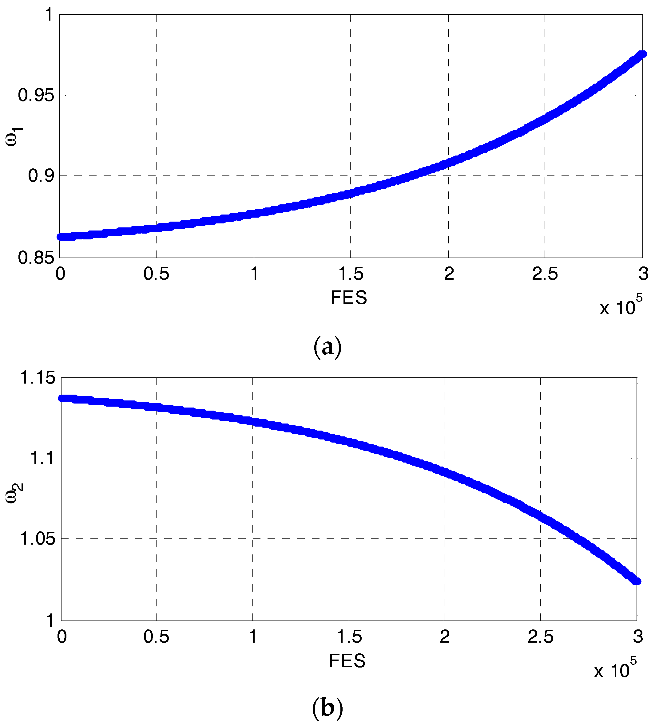
3.2. Control Parameters Assignments

In classic DE, control parameters are preset and fixed during the entire iteration process. However, it is impossible to find one constant parameter setting that can fit all problems. As pointed out in [53], the different parameter settings not only play an important role in the performance of DE, but also may be used to solve specific test problems. Thus, a novel parameter adaptation scheme is presented to adjust the parameter F and Cr at different evolutionary stage.

In MCPDE algorithm, the parameter settings are divided into three stages according to the successful mutation factors F at current generation. The initial F_i and Cr_i used by each cloud particle $x_i$ are generated independently and formulated as follows, respectively:

$$F_i=r_2\times (r_1\times \frac{f_0}{5\sqrt{MaxFES}}+\frac{f_0}{5})+f_0$$

(9)

$$C{r}_i=r_2\times (r_1\times \frac{c{r}_0}{5\sqrt{MaxFES}}+\frac{c{r}_0}{5})+c{r}_0$$

(10)

where f₀ and cr₀ are initialized to be 0.5, respectively. r₁ and r₂ are random numbers in [0, 1].

In each generation, the set S_F is used to store all successful mutation factors at current generation. Similarly, the set S_Cr stores all the successful crossover rates at current generation. The size of S_F is recorded as |S_F|. If |S_F| exceeds the current population size N, randomly selected elements are deleted from S_F and S_Cr. Then S_F and S_Cr are preserved for the next generation. When the set S_F is empty, it indicates that F and Cr at current generation are the proper parameters for the algorithm. Then, they are preserved for the next generation. When |S_F| is less than the current population size N, new control parameters $F_1^{\text{'}},F_2^{\text{'}},\cdots , F_{N-\left|S_F\right|}^{\text{'}}$ are produced according to Equation (9). $C{r}_1^{\text{'}},C{r}_2^{\text{'}},\cdots ,C{r}_{N-\left|S_F\right|}^{\text{'}}$ are defined by

$$C{r}_i^{\text{'}}=\mathsf{\sigma }\left({\mathrm{S}}_{Cr}\right)+r_i \left(i=1,\cdots ,N-\left|S_{Cr}\right|\right)$$

(11)

where $\mathsf{\sigma }\left({\mathrm{S}}_{Cr}\right)$ refers to the standard deviation of ${\mathrm{S}}_{Cr}$. $r_i$ is randomly selected in the range [0, 1].

By the end of each generation, the parameters F and Cr are updated when |S_F| is less than the current population size N, as defined by

$$F={\mathrm{S}}_F{\displaystyle \cup }{F}^{\prime }$$

(12)

$$Cr={\mathrm{S}}_{Cr}{\displaystyle \cup }C{r}^{\text{'}}$$

(13)

where $F^{\prime }=(F_1^{\text{'}},F_2^{\text{'}},\cdots ,F_{N-\left|S_F\right|}^{\text{'}})$, $C{r}^{\text{'}}=(C{r}_1^{\text{'}},C{r}_2^{\text{'}},\cdots ,C{r}_{N-\left|S_F\right|}^{\text{'}})$.

In MCPDE algorithm, different control parameters are chosen at different stages. At the early stage of evolution, the control parameter values near f₀ and cr₀ with the randomization according to Equations (9) and (10). Better diversity may improve the exploration ability. Then, cloud particles try to explore further areas in the solution space. At each generation, better control parameters are preserved for the next generation. The population diversity is improved and the convergence speed is accelerated with better control parameters. However, it is difficult to find better control parameters with the increasing generation. Thus, the algorithm may hard to jump out of the local optimum because of faster convergence and poorer diversity. In order to solve these problems, some new parameters F are introduced to maintain search efficiency according to Equations (9) and (12) while some new parameters Cr are produced to improve population diversity according to Equations (11) and (13). Therefore, the performance of the algorithm MCPDE is improved by choosing different control parameters strategies at different evolutionary stages.

The size of the population used by EAs plays a significant role in controlling exploration and exploitation. Large population sizes can encourage wider exploration of the search space, while small population sizes may promote exploitation of the search space. Therefore, the population size is gradually decreased as the iteration continues. By the end of each generation, the population size N is updated and is defined by

$$N^{\prime }=N_0-\frac{N_0}{MaxFES}\times FES$$

(14)

$$N=\{\begin{array}{ll}N-1& if N<N^{\prime }\\ N& otherwise\end{array}$$

(15)

where N₀ is the initial population size. FES is the current number of fitness evaluation, and MaxFES is the maximum number of fitness evaluations. If $N< N^{\text{'}}$, the worst individual is deleted and the archive size is resized. Because Equation (7) requires at least four particles, the minimum population size N is set to 4.

3.3. Orthogonal Crossover

It is well known that crossover operation is helpful for sharing the better gene segment by exchanging the gene information of the parents. However, the quality of the offspring produced by the crossover operator is highly dependent on the characteristics of target problems, so that multiple crossover operators are employed instead of a single crossover operator for solving different optimization problems [54]. As pointed out in [55], OX (orthogonal crossover) operators can conduct effective search in a region proposed by the parents. Hence, we come up with the idea that uses QOX (quantization technique with orthogonal crossover) [55] operator to enhance the search ability of MCPDE. In order to save the computational cost, we apply QOX only on a better particle which is randomly selected from $P_{best,G}$. The orthogonal array used in QOX operator is often denoted by $L_M\left(Q^K\right)$, namely K factors (i.e., variables) with Q levels (i.e., values) and M combinations. In MCPDE, let Q = 3, M = 9, and then $L_9\left(3^4\right)$ is used.

$$L_9\left(3^4\right)=\left[\begin{array}{c}1 1 1 1\\ 1 2 2 2\\ 1 3 3 3\\ 2 1 2 3\\ 2 2 3 1\\ 2 3 1 2\\ 3 1 3 2\\ 3 2 1 3\\ 3 3 2 1\end{array}\right]$$

(16)

Q levels for the cloud particle $P_{i,G}$ is defined as follows:

$$l_{i,j}=\min \left(C_{i,G}^{best},C_{i,G} \right)+\frac{j-1}{Q-1}\times \left(\max \left(C_{i,G}^{best},C_{i,G}\right)-\min \left(C_{i,G}^{best},C_{i,G}\right)\right)$$

(17)

where j = 1, …, Q. $C_{i,G}^{best}$ and $C_{i,G}$ are the parents which define a search range [$\min \left(C_{i,G}^{best},C_{i,G}\right)$, $\max \left(C_{i,G}^{best},C_{i,G}\right)$] for particle $P_{i,G}$. $C_{i,G}^{best}$ is randomly selected from $P_{best,G}$.

The particle $P_{i,G}$ is divided into K subvectors:

$$\{\begin{array}{l}{H}_1=\left(p_{i,G}^1,p_{i,G}^2,\cdots ,p_{i,G}^{t_1}\right)\\ H_2=\left(p_{i,G}^{t_1+1},p_{i,G}^{t_1+2},\cdots ,p_{i,G}^{t_2}\right)\\ \cdots \\ H_k=\left(p_{i,G}^{t_{k-1}+1},p_{i,G}^{t_{k-1}+2},\cdots ,p_{i,G}^D\right)\end{array}$$

(18)

where t₁, t₂, …, t_k−1 are randomly generated integers and 1 < t₁ < t₂ < t_k−1 <…< D.

H_i is treated as a factor in QOX operator, and Q levels for are H_i defined as follows:

$$\{\begin{array}{l}{L}_{i1}=\left(l_{t_{i-1}+1,1},l_{t_{i-1}+2,1},\cdots ,l_{t_i,1}\right) \\ L_{i2}=\left(l_{t_{i-1}+1,2},l_{t_{i-1}+2,2},\cdots ,l_{t_i,2}\right)\\ \cdots \\ L_{iQ}=\left(l_{t_{i-1}+1,Q},l_{t_{i-1}+2,Q},\cdots ,l_{t_i,Q}\right) \end{array}$$

(19)

Then, M solutions are constructed on factors H₁, H₂, …, H_k.

The pseudo-code of MCPDE is illustrated in Algorithm 1.

Algorithm 1. MCPDE Algorithm
1:	Initialize D (number of dimensions), N (number of population), $L_M\left(Q^K\right)$; Archive A = φ;
2:	Initialize population randomly
3:	Generate mutation factors F and Cr according to Equations (9) and (10)
4:	while the termination criteria are not met do
5:	Randomly replace N/D inferior solutions by their opposite solutions according to Equation (8)
6:	Generate new individuals according to Equations (5)–(7)
7:	Randomly select an index i from {1, …, N}
8:	Qrthogonal Crossover according to Equations (17)–(19)
9:	for i = 1 to N do
10:	if f(ui) < f(xi) then
11:	xi → A; xi = ui
12:	endif
13:	endfor
14:	Calcute N for the next generation according to Equations (14) and (15)
15:	if |SF| ≥ N then
16:	delete randomly selected elements from the SF and SCr so that the parameters size are N
17:	elseif (|SF| < N and SF ≠ φ) then
18:	Update F and Cr are according to Equations (11)–(13)
19:	elseif SF = φ then
20:	Fg+1 = Fg; Crg+1 = Crg;
21:	endif
22:	endwhile

4. Experiments and Discussion

4.1. General Experimental Setting

(1) Test Problems and Dimension Setting: For a comprehensive evaluation of MCPDE, all the CEC2013 [36] benchmark functions are used to evaluate the performance of MCPDE. The CEC2013 benchmark set consists of 28 test functions. According to their shape characteristics, these benchmark functions can be broadly classified into three kinds of optimization functions [56].

• unimodal problems f₁–f₅
• basic multimodal problems f₆–f₂₀, and
• composition problems f₂₁–f₂₈

For all of the problems, the search space is [–100,100]^D. In this paper, the dimension (D) of all functions is set to 10 and 30.

(2) Experimental Platform and Termination Criterion: For all experiments, 30 independent runs are carried out on the same machine with a Celoron 3.40 GHz CPU, 4 GB memory, and windows 7 operating system with Matlab R2009b, and conducted with D × 10,000 (number of function evaluations, FES).

(3) Performance Metrics: In our experimental studies, the mean value (F_mean), standard deviation (SD), maximum value (Max) and minimum value (Min) of the solution error measure [57] which is defined as f(x)$-$f(x^*) are recorded for evaluating the performance of each algorithm, where f(x) is the best fitness value found by an algorithm in a run, and f(x^*) is the real global optimization value of tested problem. In order to statistically compare the proposed algorithm with its peers, Wilcoxon’s rank-sum test at the 5% significance level is used to evaluate whether the median fitness values of two sets of obtained results are statistically different from each other. Three marks “−”, “+” and “≈” are also used to denote that the performance of MCPDE is better than, worse than, and similar to that of the compared algorithm, respectively.

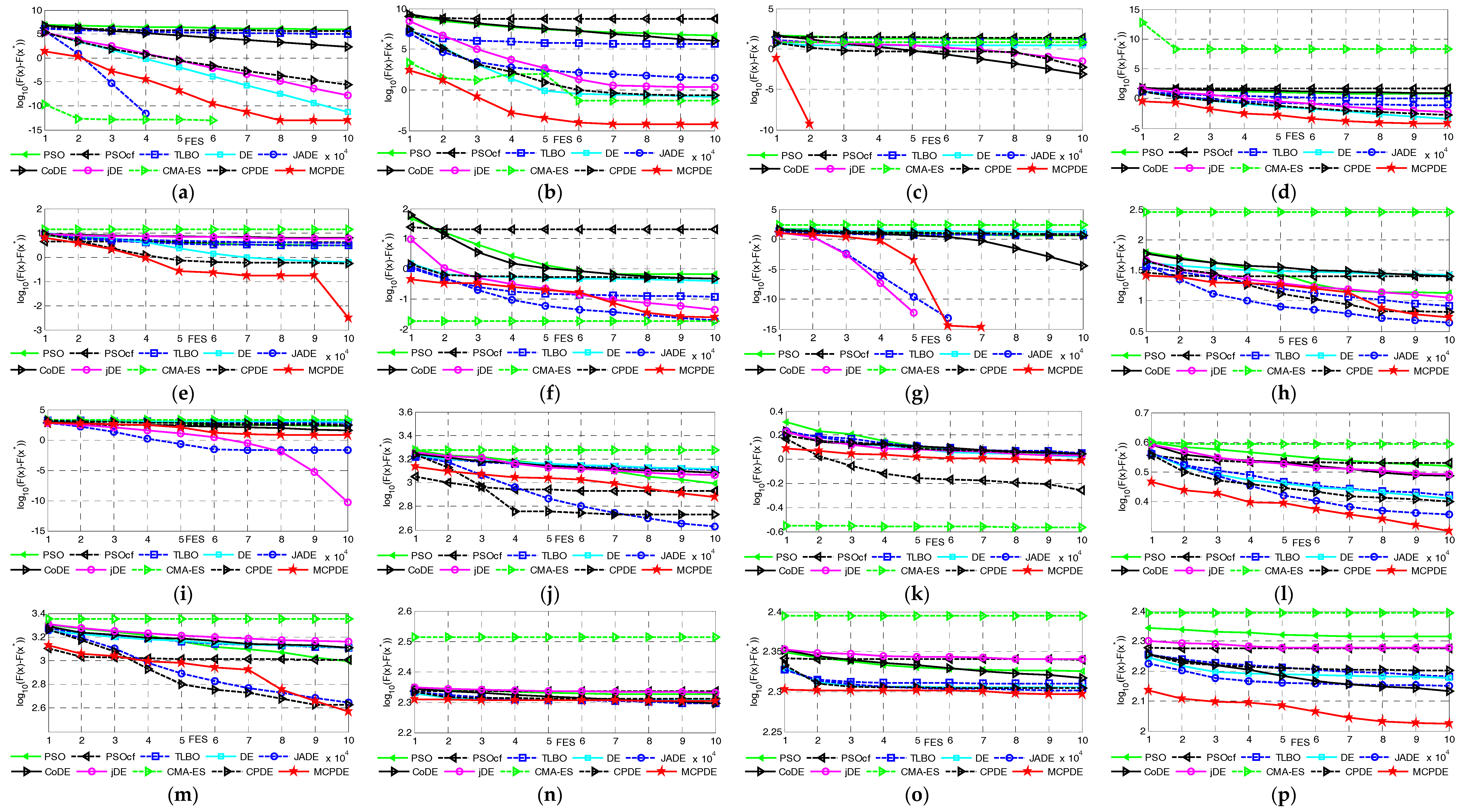
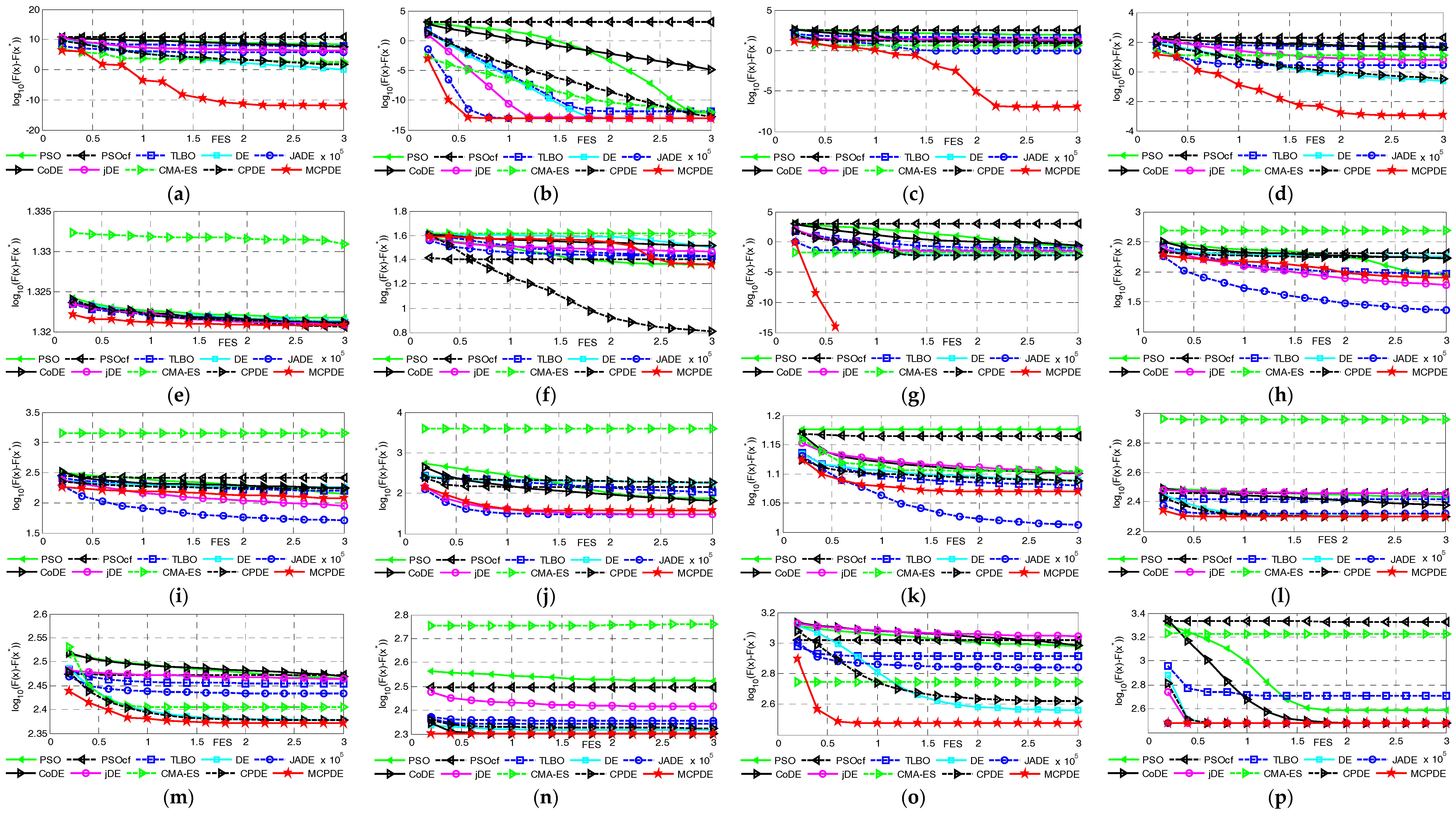
4.2. Comparison with Nine State-of-the-Art Intelligent Algorithms on 10 and 30 Dimension

In this part, MCPDE is compared with PSO, PSOcf (PSO with constriction factor) [58], TLBO, DE, JADE, CoDE, jDE, CMA-ES and CPDE. The appropriate parameters are important for the performance of the intelligent optimization algorithms. Therefore, the setting of parameters of different algorithms is given in the following:

For MCPDE, The population size N is set to 13 × D. The maximum size of the archive is set to 1.5 × N. For DE, the population size N is set to 100. F and CR are set to 0.5 and 0.9, respectively. For PSO, the population size N is set to 40, the linearly decreasing inertia ω from 0.9 to 0.4 is adopted over the course of the search, and the acceleration coefficients c₁, c₂ are both set to 1.49445. For JADE, the population size N is set to 100, p = 0.05 and c = 0.1. The parameters of other algorithms are the same as those used in the corresponding references.

The statistical results, in terms of F_mean, SD, Max and Min obtained in 30 independent runs by each algorithm, are reported in

Table 1. Experimental results of PSO, PSOcf, TLBO, DE, JADE, CoDE, jDE, CMA-ES, CPDE and MCPDE over 30 independent runs on f₁–f₅ test functions with 10D.

F		PSO	PSOcf	TLBO	DE	JADE	CoDE	jDE	CMA-ES	CPDE	MCPDE
f1	Fmean	5.30 × 10−14	31.2	3.03 × 10−14	0	0	1.80 × 10−11	0	0	0	0
	SD	9.78 × 10−14	171	7.86 × 10−14	0	0	7.98 × 10−12	0	0	0	0
	Max	2.27 × 10−14	938	2.27 × 10−13	0	0	3.66 × 10−11	0	0	0	0
	Min	0	0	0	0	0	5.45 × 10−12	0	0	0	0
Compare/Rank		−/8	−/10	−/7	≈/1	≈/1	−/9	≈/1	≈/1	≈/1	\/1
f2	Fmean	9.59 × 105	5.00 × 105	1.06 × 105	5.98 × 10−12	0	198	1.61 × 10−8	0	3.04 × 10−6	9.85 × 10−14
	SD	9.33 × 105	5.85 × 105	9.08 × 104	4.39 × 10−12	0	89	7.90 × 10−8	0	1.61 × 10−6	1.14 × 10−13
	Max	3.48 × 106	2.36 × 106	3.87 × 105	2.18 × 10−11	0	425	4.33 × 10−7	0	6.71 × 10−6	2.27 × 10−13
	Min	9.70 × 104	3.02 × 104	1.58 × 104	1.13 × 10−12	0	61.6	0	0	6.78 × 10−7	0
Compare/Rank		−/10	−/9	−/8	−/4	+/1	−/7	−/5	+/1	−/6	\/3
f3	Fmean	4.66 × 106	4.99 × 108	4.82 × 105	0.135	26.8	1.05 × 106	2.15	4.35 × 10−2	0.194	6.34 × 10−5
	SD	1.39 × 107	8.24 × 108	1.98 × 106	0.174	35.8	7.04 × 105	3.70	0.238	0.288	4.82 × 10−5
	Max	7.39 × 107	3.62 × 109	1.07 × 107	0.688	116	2.65 × 106	15.1	1.30	1.15	1.42 × 10−4
	Min	4.67 × 10−3	8.16 × 105	2.29 × 10−2	1.06 × 10−9	0	9.83 × 104	8.73 × 10−4	0	1.21 × 10−5	2.27 × 10−13
Compare/Rank		−/9	−/10	−/7	−/3	−/6	−/8	−/5	−/2	−/4	\/1
f4	Fmean	3.87 × 103	2.05 × 103	2.98 × 103	7.57 × 10−14	320	9.83 × 10−1	3.72 × 10−12	0	0	0
	SD	3.40 × 103	3.80 × 103	1.23 × 103	1.24 × 10−13	1.26 × 103	4.45 × 10−1	1.28 × 10−11	0	0	0
	Max	1.85 × 104	2.12 × 104	6.90 × 103	4.54 × 10−13	6.04 × 103	1.89	6.91 × 10−11	0	0	0
	Min	334	104	1.38 × 103	0	0	2.61 × 10−1	0	0	0	0
Compare/Rank		−/10	−/8	−/9	−/4	−/7	−/6	−/5	≈/1	≈/1	\/1
f5	Fmean	1.21 × 10−13	18.2	1.47 × 10−13	0	0	5.17 × 10−8	0	2.08 × 10−13	0	0
	SD	5.92 × 10−14	42.2	6.08 × 10−14	0	0	1.88 × 10−8	0	1.12 × 10−13	0	0
	Max	2.27 × 10−13	136	3.41 × 10−13	0	0	1.04 × 10−7	0	6.82 × 10−13	0	0
	Min	0	1.13 × 10−13	1.13 × 10−13	0	0	1.45 × 10−8	0	1.13 × 10−13	0	0
Compare/Rank		−/6	−/10	−/7	≈/1	≈/1	−/9	≈/1	−/8	≈/1	\/1
−/≈/+		5/0/0	5/0/0	5/0/0	3/2/0	2/2/1	5/0/0	3/2/0	2/2/1	2/3/0	\
Avg-Rank		8.60	9.40	7.60	2.60	3.20	7.80	3.40	2.60	2.60	1.40

and

Table 2. Experimental results of PSO, PSOcf, TLBO, DE, JADE, CoDE, jDE, CMA-ES, CPDE and MCPDE over 30 independent runs on f₁–f₅ test functions with 30D.

F		PSO	PSOcf	TLBO	DE	JADE	CoDE	jDE	CMA-ES	CPDE	MCPDE
f1	Fmean	6.29 × 10−13	7.90 × 103	1.11 × 10−12	0	0	3.63 × 10−8	0	4.32 × 10−13	2.27 × 10−14	0
	SD	2.78 × 10−13	3.56 × 103	6.49 × 10−13	0	0	1.18 × 10−8	0	1.92 × 10−13	6.99 × 10−14	0
	Max	1.81 × 10−12	1.97 × 104	3.63 × 10−12	0	0	6.32 × 10−8	0	9.09 × 10−13	2.27 × 10−13	0
	Min	2.27 × 10−13	2.70 × 103	4.54 × 10−13	0	0	1.26 × 10−8	0	2.27 × 10−13	0	0
Compare/Rank		−/7	−/10	−/8	≈/1	≈/1	−/9	≈/1	−/6	≈/1	\/1
f2	Fmean	1.51 × 107	3.91 × 107	1.23 × 106	3.47 × 105	6.25 × 103	1.24 × 105	2.26 × 105	4.32 × 10−13	2.97 × 105	344
	SD	1.12 × 107	4.06 × 107	5.38 × 105	2.59 × 105	6.93 × 103	1.40 × 105	1.59 × 105	1.61 × 10−13	2.04 × 105	252
	Max	4.32 × 107	1.43 × 108	2.31 × 106	9.68 × 105	3.43 × 104	7.28 × 105	7.46 × 105	6.82 × 10−13	7.35 × 105	951
	Min	7.68 × 105	2.30 × 106	2.41 × 105	4.85 × 104	545	2.42 × 104	5.69 × 104	2.27 × 10−13	8.34 × 104	21.4
Compare/Rank		−/9	−/10	−/8	−/7	−/3	−/4	−/5	+/1	−/6	\/2
f3	Fmean	2.64 × 108	5.51 × 1010	5.44 × 107	1.22	6.46 × 105	2.88 × 107	1.53 × 106	263	44.7	1.31 × 10−12
	SD	5.76 × 108	3.91 × 1010	8.74 × 107	5.22	1.97 × 106	1.40 × 107	3.19 × 106	1.01 × 103	167	2.61 × 10−12
	Max	2.89 × 109	1.51 × 1011	2.99 × 108	28.5	9.62 × 106	7.14 × 107	1.28 × 107	5.42 × 103	753	1.11 × 10−11
	Min	3.57 × 106	5.18 × 109	6.45 × 105	2.14 × 10−7	7.50 × 10−12	7.79 × 106	2.83 × 10−1	2.04 × 10−12	1.52 × 10−2	0
Compare/Rank		−/9	−/10	−/8	−/2	−/5	−/7	−/6	−/4	−/3	\/1
f4	Fmean	7.34 × 103	4.68 × 103	8.05 × 103	1.32 × 103	1.03 × 104	17.8	4.90	3.94 × 10−13	776	3.91 × 10−3
	SD	2.77 × 103	3.98 × 103	2.60 × 103	840	1.67 × 104	14.2	4.37	1.57 × 10−13	303	5.19 × 10−3
	Max	1.60 × 104	1.67 × 104	1.46 × 104	3.61 × 103	5.57 × 104	60.5	19.7	6.82 × 10−13	1.51 × 103	1.55 × 10−2
	Min	3.13 × 103	1.03 × 103	3.32 × 103	302	5.03 × 10−8	3.17	4.61 × 10−1	2.27 × 10−13	364	1.30 × 10−4
Compare/Rank		−/8	−/7	−/9	−/6	−/10	−/4	−/3	+/1	−/5	\/2
f5	Fmean	7.50 × 10−13	1.29 × 103	1.44 × 10−12	9.47 × 10−14	9.09 × 10−14	1.35 × 10−5	9.09 × 10−14	9.32 × 10−13	1.53 × 10−13	9.47 × 10−14
	SD	5.11 × 10−13	962	7.16 × 10−13	4.30 × 10−14	4.62 × 10−14	3.73 × 10−6	4.62 × 10−14	1.74 × 10−12	5.56 × 10−14	4.30 × 10−14
	Max	2.27 × 10−12	3.31 × 103	4.32 × 10−12	1.13 × 10−13	1.13 × 10−13	2.26 × 10−5	1.13 × 10−13	7.73 × 10−12	2.27 × 10−13	1.13 × 10−13
	Min	3.41 × 10−13	191	6.82 × 10−13	0	0	7.04 × 10−6	0	2.27 × 10−13	1.13 × 10−13	0
Compare/Rank		−/6	−/10	−/8	≈/1	≈/1	−/9	≈/1	−/7	−/5	\/1
−/≈/+		5/0/0	5/0/0	5/0/0	3/2/0	3/2/0	5/0/0	3/2/0	3/0/2	4/1/0	\
Avg-Rank		7.80	9.40	8.20	3.40	4.00	6.60	3.20	3.80	4.00	1.40

.

(1) Unimodal problems f₁–f₅: From the statistical results of Table 1 and Table 2, we can see that MCPDE is better than other compared algorithms on unimodal problems f₁–f₅ according to the average rank (Avg-rank) for 10 dimensions and 30 dimensions. Considering f₁–f₅ with 10 dimensions, for f₁, MCPDE, DE, JADE, jDE, CMA-ES and CPDE work well and obtain better results. For f₂, MCPDE performs better than other algorithms except JADE and CMA-ES. Moreover, for f₃, MCPDE performs significantly better than the compared algorithms. For f₄, MCPDE, CMA-ES and CPDE beat other compared algorithms. For f₅, MCPDE, DE, JADE, jDE and CPDE are better than other algorithms. On f₁–f₅, MCPDE performs better than PSO, PSOcf, TLBO, DE, JADE, CoDE, jDE, CMA-ES and CPDE on 5, 5, 5, 3, 2, 5, 3, 2, 2 test problems, respectively. The overall ranking sequences for unimodal problems are MCPDE, CMA-ES, DE, CPDE, JADE, jDE, TLBO, CoDE, PSO and PSOcf in descending direction. When the search space dimension D is set to 30, according to Table 2, MCPDE is much better than PSO, PSOcf, TLBO, DE, JADE, CoDE, jDE, CMA-ES and CPDE on 5, 5, 5, 3, 3, 5, 3, 3, 4 test functions, respectively. MCPDE performs better than all compared algorithms for the unimodal problems except f₂ and f₄. For f₂ and f₄, MCPDE ranks secondly. The overall ranking sequences for unimodal problems are MCPDE, jDE, DE, CMA-ES, JADE, CPDE, CoDE, PSO, TLBO and PSOcf in descending direction. The reason that MCPDE has the outstanding performance may be the use of the inertia factors, which are helpful for guiding the search direction.

(2) Multimodal problems f₆–f₂₀: Considering the multimodal functions f₆–f₂₀ in

Table 3. Experimental results of PSO, PSOcf, TLBO, DE, JADE, CoDE, jDE, CMA-ES, CPDE and MCPDE over 30 independent runs on f₆–f₂₀ test functions with 10D.

F		PSO	PSOcf	TLBO	DE	JADE	CoDE	jDE	CMA-ES	CPDE	MCPDE
f6	Fmean	16.6	26.5	6.64	2.61	6.21	8.43 × 10−4	3.19 × 10−2	7.01	5.67 × 10−3	0
	SD	24.9	27.3	4.57	4.41	4.80	2.93 × 10−4	4.26 × 10−2	4.41	2.53 × 10−2	0
	Max	96.8	90.8	9.81	9.81	9.81	1.42 × 10−3	2.04 × 10−1	9.81	1.13 × 10−1	0
	Min	2.06 × 10−1	9.81	2.05 × 10−3	0	0	1.75 × 10−4	3.31 × 10−4	0	2.72 × 10−12	0
Compare/Rank		−/9	−/10	−/7	−/5	−/6	−/2	−/4	−/8	−/3	\/1
f7	Fmean	5.56	46.3	1.07	3.43 × 10−4	7.97 × 10−2	8.29	4.96 × 10−3	2.07 × 108	1.48 × 10−3	7.58 × 10−5
	SD	5.33	26.4	3.17	2.50 × 10−4	1.17 × 10−1	1.93	5.68 × 10−3	1.13 × 109	1.45 × 10−3	1.00 × 10−4
	Max	20.5	117	17.1	9.58 × 10−4	4.81 × 10−1	12.8	2.00 × 10−2	6.21 × 109	5.79 × 10−3	3.65 × 10−4
	Min	3.80 × 10−1	8.06	1.90 × 10−4	2.98 × 10−5	2.04 × 10−8	4.30	9.58 × 10−5	1.09	3.73 × 10−4	6.56 × 10−8
Compare/Rank		−/7	−/9	−/6	−/2	−/5	−/8	−/4	−/10	−/3	\/1
f8	Fmean	20.3	20.3	20.3	20.3	20.3	20.3	20.3	20.3	20.3	20.3
	SD	8.88 × 10−2	8.26 × 10−2	5.93 × 10−2	8.49 × 10−2	8.25 × 10−2	7.42 × 10−2	6.74 × 10−2	4.55 × 10−1	7.43 × 10−2	7.12 × 10−2
	Max	20.5	20.4	20.4	20.4	20.5	20.4	20.4	21.6	20.4	20.4
	Min	20.1	20.1	20.2	20	20.1	20.1	20.1	20	20.2	20.1
Compare/Rank		≈/1	≈/1	≈/1	≈/1	≈/1	≈/1	≈/1	−/10	≈/1	\/1
f9	Fmean	3.11	4.21	2.95	6.20 × 10−1	3.74	6.06	5.76	14.1	5.60 × 10−1	1.66 × 10−1
	SD	1.54	1.65	8.69 × 10−1	7.40 × 10−1	7.45 × 10−1	6.31 × 10−1	6.96 × 10−1	3.72	6.41 × 10−1	3.23 × 10−1
	Max	6.99	7.01	4.35	2.24	4.98	7.04	7.04	20.3	2.39	9.78 × 10−1
	Min	2.65 × 10−1	8.70 × 10−1	1.19	6.92 × 10−8	1.89	4.61	4.50	7.71	2.60 × 10−4	0
Compare/Rank		−/5	−/7	−/4	−/3	−/6	−/9	−/8	−/10	−/2	\/1
f10	Fmean	6.52 × 10−1	20.7	1.16 × 10−1	3.91 × 10−1	1.95 × 10−2	4.59 × 10−1	4.47 × 10−2	1.83 × 10−2	4.82 × 10−1	2.51 × 10−2
	SD	4.56 × 10−1	35.8	5.60 × 10−2	1.45 × 10−1	1.04 × 10−2	5.96 × 10−2	3.71 × 10−2	3.20 × 10−2	9.18 × 10−2	1.08 × 10−2
	Max	1.86	165	2.26 × 10−1	5.57 × 10−1	4.03 × 10−2	5.57 × 10−1	1.48 × 10−1	1.75 × 10−1	6.30 × 10−1	4.18 × 10−2
	Min	1.08 × 10−1	1.72 × 10−2	2.27 × 10−2	1.72 × 10−2	2.26 × 10−3	3.32 × 10−1	2.56 × 10−9	0	3.10 × 10−1	5.68 × 10−14
Compare/Rank		−/9	−/10	−/5	−/6	+/2	−/7	≈/3	+/1	−/8	\/3
f11	Fmean	3.78	8.29	5.29	16.7	0	3.41 × 10−5	0	286	3.79	0
	SD	2.11	9.65	2.33	3.81	0	2.87 × 10−5	0	331	3.14	0
	Max	7.95	39.4	9.94	23.8	0	1.40 × 10−4	0	921	9.35	0
	Min	9.94 × 10−1	0	1.99	9.08	0	3.73 × 10−6	0	3.97	2.43 × 10−8	0
Compare/Rank		−/5	−/8	−/7	−/9	≈/1	−/4	≈/1	−/10	−/6	\/1
f12	Fmean	13.5	25	8.18	26.8	4.38	25	11.4	284	6.57	5.36
	SD	5.23	12	3.64	4.25	1.22	5.15	3.22	327	4.06	1.75
	Max	22.8	54.1	14.8	35.5	7.07	33.4	19	1.37 × 103	19.1	8.66
	Min	4.97	6.96	1.25	17.3	1.83	11	5.20	5.96	1.98	1.52
Compare/Rank		−/6	−/7	−/4	−/9	≈/1	−/7	−/5	−/10	≈/2	\/2
f13	Fmean	22.1	33.5	11.6	24.7	5.27	26.6	14.8	311	7.92	6.69
	SD	7.35	11.3	5.08	3.85	2.39	4.31	3.84	412	4.50	2.83
	Max	40.1	55.9	25.6	31.8	11.5	32.6	22.4	1.36 × 103	16.5	13.5
	Min	7.22	3.45	3.55	16.5	2.45	13.7	6.73	12.6	2.03	1.98
Compare/Rank		−/6	−/9	−/4	−/7	+/1	−/8	−/5	−/10	≈/2	\/2
f14	Fmean	226	236	598	995	2.28 × 10−2	38.8	4.74 × 10−11	1.80 × 103	275	6.97
	SD	161	157	256	136	3.47 × 10-2	7.97	1.83 × 10-10	423	115	4.94
	Max	605	667	1.09 × 103	1.17 × 103	1.24 × 10-1	53.2	9.72 × 10-10	2.80 × 103	506	15.1
	Min	3.47	3.60	32.3	472	0	19.3	0	993	72.3	6.24 × 10-2
Compare/Rank		−/5	−/6	−/8	−/9	−/2	−/4	+/1	−/10	−/7	\/3
f15	Fmean	982	847	1.28 × 103	1.31 × 103	426	1.20 × 103	1.15 × 103	1.88 × 103	535	760
	SD	345	231	188	155	109	141	151	438	195	142
	Max	1.55 × 103	1.27 × 103	1.56 × 103	1.53 × 103	653	1.46 × 103	1.48 × 103	2.75 × 103	772	983
	Min	290	187	743	809	189	963	901	1.00 × 103	113	479
Compare/Rank		−/5	−/4	−/8	−/9	+/1	−/7	−/6	−/10	+/2	\/3
f16	Fmean	1.09	5.56 × 10−1	1.13	1.04	1.11	1.10	1.07	2.72 × 10−1	1.10	9.92 × 10−1
	SD	2.88 × 10−1	1.80 × 10−1	2.43 × 10−1	2.39 × 10−1	2.07 × 10−1	2.12 × 10−1	1.82 × 10−1	2.55 × 10−1	2.05 × 10−1	1.04 × 10−1
	Max	1.72	9.09 × 10−1	1.60	1.50	1.45	1.54	1.39	1.23	1.41	1.14
	Min	4.49 × 10−1	2.50 × 10−1	6.79 × 10−1	5.48 × 10−1	6.63 × 10−1	6.40 × 10−1	7.12 × 10−1	3.62 × 10−2	5.14 × 10−1	7.16 × 10−1
Compare/Rank		−/6	+/2	−/10	≈/3	−/9	−/7	−/5	+/1	−/7	\/3
f17	Fmean	14.2	13.3	24.7	27.7	10.1	11.4	10.1	956	28	10.3
	SD	4.68	1.46	3.31	3.28	1.44 × 10−14	5.07 × 10−1	2.05 × 10−10	469	2.80	3.33 × 10−1
	Max	21.7	17.9	34.4	35.7	10.1	12.3	10.1	1.58 × 103	33.9	11.3
	Min	4.06	11	18.2	22.2	10.1	9.56	10.1	22.4	23.6	10.1
Compare/Rank		≈/4	≈/4	−/7	−/8	+/1	+/4	+/1	−/10	−/9	\/3
f18	Fmean	34.6	21.8	32.6	36.1	18.8	42.2	31.1	925	36.3	25.9
	SD	10.7	7.60	4.00	3.85	2.24	5.46	3.32	462	3.30	4.38
	Max	54.2	40.2	41.5	42.9	22.9	52.2	36.5	1.85 × 103	42.6	32.7
	Min	5.60	7.21	25.6	26.9	15.4	31.8	23.6	15.1	30.8	15.6
Compare/Rank		−/6	+/2	−/5	−/7	+/1	−/9	−/4	−/10	−/8	\/3
f19	Fmean	6.33 × 10−1	1.99	9.83 × 10−1	2.17	3.37 × 10−1	9.24 × 10−1	4.00 × 10−1	1.10	1.95	4.44 × 10−1
	SD	1.78 × 10−1	5.08	2.24 × 10−1	3.47 × 10−1	4.32 × 10−2	1.49 × 10−1	9.80 × 10−2	4.74 × 10−1	3.22 × 10−1	1.05 × 10−1
	Max	1.00	20.9	1.35	2.66	3.94 × 10−1	1.24	5.74 × 10−1	2.52	2.34	6.60 × 10−1
	Min	2.99 × 10−1	3.66 × 10−1	5.86 × 10−1	9.78 × 10−1	2.08 × 10−1	5.82 × 10−1	1.48 × 10−1	3.99 × 10−1	1.25	2.39 × 10−1
Compare/Rank		≈/3	−/9	−/7	−/10	+/1	−/6	≈/2	−/7	−/8	\/2
f20	Fmean	3.31	3.39	2.64	2.57	2.27	3.06	3.10	3.92	2.50	1.99
	SD	7.65 × 10−1	4.09 × 10−1	4.20 × 10−1	2.61 × 10−1	4.49 × 10−1	2.37 × 10−1	1.75 × 10−1	4.20 × 10−1	2.77 × 10−1	1.87 × 10−1
	Max	5.00	4.01	3.32	3.29	3.23	3.39	3.45	4.99	3.07	2.24
	Min	1.97	2.26	1.83	1.93	1.72	2.58	2.73	2.92	2.09	1.55
Compare/Rank		−/8	−/9	−/5	−/4	≈/1	−/6	−/7	−/10	−/3	\/1
−/≈/+		14/1/0	12/1/2	14/1/0	14/1/0	4/3/8	14/1/0	9/4/2	13/0/2	11/3/1	\
Avg-Rank		5.67	6.47	5.87	6.20	2.60	5.93	3.80	8.47	4.73	2.00

, MCPDE is significantly better than other algorithms on f₆, f₇, f₉ and f₂₀. Considering f₈, most of the compared algorithms can achieve the similar results except CMA-ES. MCPDE beats most of the compared algorithms except that JADE and jDE have a similar performance on f₁₁. JADE performs best on f₁₂, f₁₃, f₁₅ and f₁₈–f₁₉. jDE performs best on f₁₄. CMA-ES performs best on f₁₀ and f₁₆. JADE and jDE perform best on f₁₇. On these 15 multimodal problems, MCPDE performs better than PSO, PSOcf, TLBO, DE, JADE, CoDE, jDE, CMA-ES and CPDE on 14, 12, 14, 14, 4, 14, 9, 13 and 11 problems respectively. The overall ranking sequences on multimodal problems are MCPDE, JADE, jDE, CPDE, PSO, TLBO, CoDE, DE, PSOcf and CMA-ES in descending direction. When the search space dimension D is set to 30, according to the experimental results on 15 test problems from

Table 4. Experimental results of PSO, PSOcf, TLBO, DE, JADE, CoDE, jDE, CMA-ES, CPDE and MCPDE over 30 independent runs ON f₆–f₂₀ test functions with 30D.

F		PSO	PSOcf	TLBO	DE	JADE	CoDE	jDE	CMA-ES	CPDE	MCPDE
f6	Fmean	90.4	339	36.6	8.88	8.80 × 10−1	13.5	18.1	4.40	8.05	1.18 × 10−7
	SD	41.2	252	28.2	6.12	4.82	2.51	8.43 × 10−1	10	4.39	1.72 × 10−7
	Max	150	1.03 × 103	80.1	26.4	26.4	26.4	20.5	26.4	26.4	5.58 × 10−7
	Min	6.90	50.4	3.35	4.18 × 10−2	0	11.9	16.4	1.13 × 10−13	5.63	1.34 × 10−10
Compare/Rank		−/9	−/10	−/8	−/5	−/2	−/6	−/7	−/3	−/4	\/1
f7	Fmean	45.9	197	49.2	2.40 × 10−1	2.68	40.4	5.90	12.1	3.30 × 10−1	1.07 × 10−3
	SD	18.4	61.5	18	5.52 × 10−1	2.58	6.67	5.11	6.38	5.47 × 10−1	7.68 × 10−4
	Max	97	324	84.9	2.84	12.4	55	17.7	27.9	2.20	2.99 × 10−3
	Min	17.7	80.2	25.7	2.39 × 10−3	1.09 × 10−1	30.3	4.15 × 10−1	1.85	6.64 × 10−3	5.42 × 10−5
Compare/Rank		−/8	−/10	−/9	−/2	−/4	−/7	−/5	−/6	−/3	\/1
f8	Fmean	20.9	20.9	20.9	20.9	20.9	20.9	20.9	21.4	20.9	20.9
	SD	5.97 × 10−2	6.20 × 10−2	4.74 × 10−2	4.61 × 10−2	1.13 × 10−1	5.74 × 10−2	5.75 × 10−2	8.31 × 10−2	5.46 × 10−2	5.16 × 10−2
	Max	21	21	21	21	21	21	21	21.6	21	20.9
	Min	20.7	20.6	20.8	20.8	20.4	20.7	20.8	21.2	20.8	20.7
Compare/Rank		≈/1	≈/1	≈/1	≈/1	≈/1	≈/1	≈/1	−/10	≈/1	\/1
f9	Fmean	22.8	25.2	26.8	32	26.8	32.5	29.2	41	6.48	22.9
	SD	3.85	4.00	4.37	11.1	1.75	1.46	1.83	10.1	2.28	3.96
	Max	2.90 × 10	32.8	37.2	40.1	29.7	34.2	34	54.9	11.2	28
	Min	15.4	18.5	16.6	9.49	23.5	29.1	25.2	19.8	2.86	15
Compare/Rank		≈/2	≈/2	−/6	−/8	−/5	−/9	−/7	−/10	−/1	\/2
f10	Fmean	1.61 × 10−1	1.01 × 103	1.20 × 10−1	7.88 × 10−3	4.54 × 10−2	2.46 × 10−1	3.80 × 10−2	1.78 × 10−2	6.53 × 10−3	0
	SD	9.72 × 10−2	6.21 × 102	7.75 × 10−2	6.85 × 10−3	2.61 × 10−2	1.76 × 10−1	2.03 × 10−2	1.29 × 10−2	4.81 × 10−3	0
	Max	4.60 × 10−1	2.44 × 103	3.40 × 10−1	2.95 × 10−2	1.03 × 10−1	5.98 × 10−1	8.86 × 10−2	5.66 × 10−2	1.47 × 10−2	0
	Min	2.46 × 10−2	2.13 × 102	2.21 × 10−2	0	0	2.79 × 10−2	7.39 × 10−3	5.68 × 10−14	5.68 × 10−14	0
Compare/Rank		−/8	−/10	−/7	−/3	−/6	−/9	−/5	−/4	−/2	\/1
f11	Fmean	33.9	151	105	129	0	25.1	0	109	71	2.77
	SD	8.52	44.1	26.6	25.8	0	2.15	0	337	13.4	1.69
	Max	58.7	261	190	176	0	28.8	0	1.89 × 103	104	7.59
	Min	18.9	74.7	67.6	73	0	19	0	26.8	48.4	5.68 × 10-14
Compare/Rank		−/5	−/10	−/7	−/9	+/1	−/4	+/1	−/8	−/6	\/3
f12	Fmean	88.2	201	92.1	180	22.9	165	59.6	484	173	80.1
	SD	37.7	91.2	24.1	9.38	3.34	12.1	8.38	828	7.87	22.2
	Max	227	421	147	196	29.8	190	70.6	2.65 × 103	191	113
	Min	41.7	78.3	43.7	156	25.7	141	34.3	25.8	161	44.1
Compare/Rank		≈/3	−/9	≈/3	−/8	+/1	−/6	+/2	−/10	−/7	\/3
f13	Fmean	140	255	156	180	50.8	175	89.5	1.44 × 103	173	117
	SD	32.8	50.4	32.2	11.3	13.5	14.7	18.3	1.41 × 103	8.86	21.9
	Max	186	378	224	198	76.5	201	131	5.06 × 103	188	140
	Min	83.4	179	76.7	146	17.9	129	58.8	79.3	155	65.7
Compare/Rank		−/4	−/9	−/5	−/8	+/1	−/7	+/2	−/10	−/6	\/3
f14	Fmean	1.22 × 103	2.65 × 103	5.64 × 103	6.08 × 103	3.12 × 10−2	1.39 × 103	8.13 × 10−1	5.27 × 103	3.36 × 103	292
	SD	317	656	1.21 × 103	549	2.49 × 10−2	154	2.11	690	644	118
	Max	1.84 × 103	3.79 × 103	7.11 × 103	6.87 × 103	1.04 × 10−1	1.70 × 103	8.89	7.44 × 103	4.43 × 103	592
	Min	634	1.56 × 103	1.71 × 103	4.43 × 103	1.81 × 10−12	1.08 × 103	5.07 × 10−9	4.07 × 103	1.94 × 103	91.8
Compare/Rank		+/4	−/6	−/9	−/10	+/1	+/5	+/2	−/8	−/7	\/3
f15	Fmean	6.19 × 103	4.34 × 103	7.07 × 103	7.12 × 103	3.20 × 103	6.92 × 103	5.60 × 103	5.16 × 103	7.04 × 103	6.66 × 103
	SD	1.25 × 103	784	331	216	347	369	392	798	288	391
	Max	7.92 × 103	6.65 × 103	7.62 × 103	7.47 × 103	3.70 × 103	7.43 × 103	6.57 × 103	6.69 × 103	7.37 × 103	7.19 × 103
	Min	3.37 × 103	3.07 × 103	6.18 × 103	6.67 × 103	2.37 × 103	6.13 × 103	4.39 × 103	3.79 × 103	6.37 × 103	6.08 × 103
Compare/Rank		≈/5	+/2	−/9	−/10	+/1	−/7	+/4	+/3	−/8	\/5
f16	Fmean	2.53	1.87	2.41	2.52	2.00	2.36	2.48	8.14 × 10−2	2.50	1.92
	SD	4.26 × 10−1	4.64 × 10−1	2.88 × 10−1	3.76 × 10−1	7.07 × 10−1	2.49 × 10−1	1.69 × 10−1	5.62 × 10−2	2.94 × 10−1	1.69 × 10−1
	Max	3.34	2.66	2.92	3.07	2.96	2.90	2.76	2.85 × 10−1	3.01	2.06
	Min	1.46	7.24 × 10−1	1.64	1.32	5.95 × 10−1	1.78	2.13	1.99 × 10−2	1.54	1.23
Compare/Rank		−/10	≈/2	−/6	−/9	≈/2	−/5	−/7	+/1	−/8	\/2
f17	Fmean	74.6	142	106	180	30.4	65.1	30.4	3.88 × 103	182	37.5
	SD	19	88.5	27.1	16.3	1.05 × 10−14	3.62	1.70 × 10−6	665	18.4	2.55
	Max	105	352	173	211	30.4	71.2	30.4	5.00 × 103	213	42.3
	Min	35.7	58.9	69.8	151	30.4	56.7	30.4	2.54 × 103	146	33.6
Compare/Rank		−/5	−/7	−/6	−/8	+/1	−/4	+/1	−/10	−/9	\/3
f18	Fmean	207	156	220	212	78.3	230	161	4.08 × 103	206	187
	SD	30.2	51.7	15.5	9.55	6.43	9.76	16	911	10	10.1
	Max	268	252	253	229	94.8	248	187	5.97 × 103	223	199
	Min	140	81.9	182	193	65.5	211	133	1.76 × 103	178	155
Compare/Rank		−/6	+/2	−/8	−/7	+/1	−/9	+/3	−/10	−/5	\/4
f19	Fmean	4.43	1.83 × 103	12.4	15	1.44	8.25	1.63	3.43	14.6	2.55
	SD	1.19	3.59 × 103	5.75	8.57 × 10−1	1.18 × 10−1	8.60 × 10−1	1.48 × 10−1	8.32 × 10−1	1.15	4.83 × 10−1
	Max	6.69	1.62 × 104	26.2	16.5	1.70	9.60	1.87	5.24	16.2	3.26
	Min	2.31	5.85	5.00	13.1	1.11	6.46	1.31	1.66	12.4	1.53
Compare/Rank		−/5	−/10	−/7	−/9	+/1	−/6	+/2	−/4	−/8	\/3
f20	Fmean	15	14.5	12	12.2	10.3	12.5	12.6	12.7	12.2	11.7
	SD	0	9.53 × 10−1	3.30 × 10−1	2.38 × 10−1	6.17 × 10−1	2.28 × 10−1	3.51 × 10−1	9.28 × 10−1	3.22 × 10−1	3.37 × 10−1
	Max	15	15	12.6	12.6	11.9	13	13.3	14.3	12.7	12.1
	Min	15	11.5	11.4	11.6	9.05	12	12	10	11.3	10.6
Compare/Rank		−/10	−/9	−/3	−/4	+/1	−/6	−/7	−/8	−/5	\/2
−/≈/+		11/4/0	10/3/2	13/2/0	14/1/0	4/2/9	14/1/0	6/1/8	13/0/2	13/1/1	\
Avg-Rank		5.67	6.60	6.27	6.73	1.93	6.07	3.73	7.00	5.33	2.47

, we find that MCPDE outperforms PSO, PSOcf, TLBO, DE, JADE, CoDE, jDE, CMA-ES and on 11, 10, 13, 14, 4, 14, 6, 13, 13 testproblems, respectively. The overall ranking sequences on multimodal problems are JADE, MCPDE, jDE, CPDE, PSO, CoDE, TLBO, PSOcf, DE and CMA-ES in descending direction.

(3) Composite problems f₂₁–f₂₈: As is known to all, composite problems are very time consuming for fitness evaluation compared to others because these functions combine multiple test problems into a complex landscape. Therefore, it is extremely difficult for state-of-the-art intelligent optimization algorithms to obtain relatively ideal results. Concerning the composition functions f₂₁–f₂₈ in

Table 5. Experimental results of PSO, PSOcf, TLBO, DE, JADE, CoDE, jDE, CMA-ES, CPDE and MCPDE over 30 independent runs on f₂₁–f₂₈ test functions with 10D.

F		PSO	PSOcf	TLBO	DE	JADE	CoDE	jDE	CMA-ES	CPDE	MCPDE
f21	Fmean	360	400	400	373	393	210	400	363	365	393
	SD	85.5	2.97 × 10−13	1.58 × 10−1	69.2	36.5	54.8	2.89 × 10−13	96.4	87.5	36.5
	Max	400	400	400	400	400	400	400	400	400	400
	Min	100	400	399	200	200	100	400	100	100	200
Compare/Rank		≈/2	−/8	−/8	≈/2	≈/2	+/1	−/8	≈/2	≈/2	\/2
f22	Fmean	295	433	366	1.04 × 103	4.07	232	56	2.31 × 103	336	27.7
	SD	130	219	307	188	4.93	47.8	18.4	475	156	18.1
	Max	531	876	1.24 × 103	1.36 × 103	17.3	318	93.4	3.11 × 103	68.5	88
	Min	69.6	33.9	41.4	491	4.42 × 10-6	111	22.8	1.31 × 103	120	0
Compare/Rank		−/5	−/8	−/7	−/9	+/1	−/4	−/3	−/10	−/6	\/2
f23	Fmean	981	1.02 × 103	1.29 × 103	1.28 × 103	445	1.27 × 103	1.44 × 103	2.24 × 103	426	371
	SD	369	398	238	134	175	199	212	518	234	157
	Max	1.65 × 103	1.88 × 103	1.77 × 103	1.61 × 103	897	1.66 × 103	1.82 × 103	3.12 × 103	793	675
	Min	246	245	706	1.06 × 103	163	879	766	1.14 × 103	72.9	33.9
Compare/Rank		−/4	−/5	−/8	−/7	≈/1	−/6	−/9	−/10	≈/1	\/1
f24	Fmean	211	216	197	202	201	197	214	327	204	202
	SD	4.09	18.9	19.3	16.6	6.82	28.9	11.2	149	3.09	3.31
	Max	218	228	219	209	211	215	222	758	209	208
	Min	200	119	148	115	168	133	160	107	200	200
Compare/Rank		−/7	−/9	≈/2	−/5	≈/2	+/1	−/8	−/10	−/6	\/2
f25	Fmean	211	218	204	202	200	207	218	247	201	200
	SD	5.12	4.26	3.65	2.96	8.77	11.2	2.10	50.5	2.27	1.15
	Max	223	227	212	212	209	213	222	350	204	204
	Min	201	210	200	200	155	148	213	200	200	200
Compare/Rank		−/7	−/8	−/5	−/4	−/2	−/6	−/8	−/10	−/3	\/1
f26	Fmean	206	188	151	150	141	136	188	247	158	105
	SD	75.8	61.8	34.5	36.1	45.3	4.20	29.2	1202	42.8	2.17
	Max	321	321	200	200	200	146	200	618	200	109
	Min	110	105	103	105	102	126	106	40.1	104	100
Compare/Rank		−/9	−/7	−/5	−/4	−/3	−/2	−/7	−/10	−/6	\/1
f27	Fmean	506	562	359	323	300	344	480	360	315	300
	SD	104	72.5	82.7	61.3	4.88 × 10-1	30.8	18.4	62.8	48.8	0
	Max	635	652	534	481	302	440	512	520	481	300
	Min	300	400	300	300	300	316	435	300	300	300
Compare/Rank		−/9	−/10	−/6	−/4	−/2	−/5	−/8	−/7	−/3	\/1
f28	Fmean	320	403	308	246	293	193	286	1.00 × 103	270	300
	SD	80.6	163	90.2	89.9	36.5	101	50.7	1.07 × 103	73.2	0
	Max	664	756	579	300	300	300	300	4.00 × 103	300	300
	Min	300	300	100	100	100	100	100	300	100	300
Compare/Rank		−/8	−/9	−/7	≈/1	≈/1	≈/1	≈/1	−/10	≈/1	\/1
−/≈/+		7/0/1	8/0/0	7/1/0	6/2/0	3/4/1	5/1/2	7/1/0	7/1/0	5/3/0	\
Avg-Rank		6.38	8.00	6.00	4.50	1.75	3.25	6.50	8.63	3.50	1.38

, MCPDE performs better than PSO, PSOcf, TLBO, DE, JADE, CoDE, jDE, CMA-ES, and CPDE on 7, 8, 7, 6, 3, 5, 7, 7 and 5 out of 8 test problems, respectively. Conversely, PSO, PSOcf, TLBO, DE, JADE, CoDE, jDE, CMA-ES and CPDE surpass MCPDE on 1, 0, 0, 0, 1, 2, 0, 0 and 0 problems respectively. The overall ranking sequences of composite problems are MCPDE, JADE, CoDE, CPDE, DE, TLBO, PSO, jDE, PSOcf and CMA-ES in descending direction. It can be observed from

Table 6. Experimental results of PSO, PSOcf, TLBO, DE, JADE, CoDE, jDE, CMA-ES, CPDE and MCPDE over 30 independent runs on f₂₁–f₂₈ test functions with 30D.

F		PSO	PSOcf	TLBO	DE	JADE	CoDE	jDE	CMA-ES	CPDE	MCPDE
f21	Fmean	290	774	318	302	305	330	295	316	269	256
	SD	83.1	343	70.2	83.7	64.7	101	72.3	94.2	76.9	50.4
	Max	443	1.89 × 103	443	443	443	443	443	443	443	300
	Min	200	200	200	200	200	200	200	200	200	200
Compare/Rank		−/3	−/10	−/8	−/5	−/6	−/9	−/4	−/7	−/2	\/1
f22	Fmean	1.30 × 103	2.60 × 103	1.92 × 103	6.13 × 103	93.5	2.21 × 103	232	7.08 × 103	3.56 × 103	353
	SD	405	627	1.18 × 103	727	30.6	268	43	868	760	118
	Max	2.36 × 103	3.74 × 103	6.04 × 103	7.18 × 103	122	2.64 × 103	314	8.45 × 103	4.58 × 103	678
	Min	754	1.48 × 103	609	4.69 × 103	15.3	1.66 × 103	160	4.66 × 103	1.73 × 103	167
Compare/Rank		−/4	−/7	−/5	−/9	+/1	−/6	+/2	−/10	−/8	\/3
f23	Fmean	6.19 × 103	4.76 × 103	7.06 × 103	7.18 × 103	3.53 × 103	7.24 × 103	6.18 × 103	7.07 × 103	7.15 × 103	5.96 × 103
	SD	1.26 × 103	999	315	203	325	223	418	634	381	483
	Max	7.77 × 103	7.07 × 103	7.57 × 103	7.66 × 103	4.13 × 103	7.65 × 103	7.52 × 103	8.18 × 103	7.76 × 103	6.68 × 103
	Min	2.99 × 103	3.01 × 103	6.44 × 103	6.78 × 103	2.73 × 103	6.70 × 103	5.49 × 103	5.51 × 103	5.98 × 103	4.99 × 103
Compare/Rank		≈/3	+/2	−/6	−/9	+/1	−/10	≈/3	−/7	−/8	\/3
f24	Fmean	272	288	261	200	208	237	284	909	200	200
	SD	10.5	10	7.89	3.25	7.42	6.97	4.30	687	2.72 × 10-1	6.02 × 10-3
	Max	296	303	278	217	228	252	291	2.23 × 103	201	200
	Min	255	271	242	200	200	222	275	213	200	200
Compare/Rank		−/7	−/9	−/6	−/3	−/4	−/5	−/8	−/10	−/2	\/1
f25	Fmean	291	296	284	238	271	294	290	254	238	235
	SD	10	9.61	9.88	4.99	15.1	5.42	5.21	27.7	4.12	2.57
	Max	315	316	305	247	289	303	297	387	244	238
	Min	272	278	266	228	239	279	277	201	230	229
Compare/Rank		−/8	−/10	−/6	−/2	−/5	−/9	−/7	−/4	−/2	\/1
f26	Fmean	333	312	219	20.7	226	200	260	574	211	200
	SD	61	84.2	50	27.5	54.2	5.20 × 10-3	86.9	504	35.1	2.26 × 10-4
	Max	373	391	352	316	345	200	389	1.87 × 103	317	200
	Min	200	200	200	200	200	200	200	132	200	200
Compare/Rank		−/9	−/8	−/5	−/3	−/6	−/2	−/7	−/10	−/4	\/1
f27	Fmean	956	1.04 × 103	820	363	691	962	1.11 × 103	555	416	300
	SD	90.5	75.9	85.5 × 10	85.4	228	153	32.7	123	109	1.19 × 10-1
	Max	1.10 × 103	1.20 × 103	961	513	1.00 × 103	1.17 × 103	1.17 × 103	799	617	300
	Min	775	861	660	300	309	659	1.04 × 103	387	300	300
Compare/Rank		−/7	−/9	−/6	−/2	−/5	−/8	−/10	−/4	−/3	\/1
f28	Fmean	385	2.13 × 103	514	300	300	300	300	300	300	300
	SD	325	258	639	2.27 × 10-13	0	6.78 × 10-3	0	3.75 × 103	1.84 × 10-9	2.65 × 10-13
	Max	1.63 × 103	2.84 × 103	2.69 × 103	300	300	300	300	1.34 × 104	300	300
	Min	300	1.67 × 103	100	300	300	300	300	100	300	300
Compare/Rank		−/7	−/10	−/8	≈/1	≈/1	−/6	≈/1	−/9	≈/1	\/1
−/≈/+		7/1/0	7/0/1	8/0/0	7/1/0	5/1/2	8/0/0	5/2/1	8/0/0	7/1/0	\
Avg-Rank		6.00	8.13	6.25	4.25	3.63	6.88	5.25	7.63	3.75	1.50

that MCPDE still performs better on these composition functions when the search space dimension D is set to 30. MCPDE performs better than PSO, PSOcf, TLBO, DE, JADE, CoDE, jDE, CMA-ES and CPDE on 7, 7, 8, 7, 5, 8, 5, 8 and 7 out of 8 test problems, respectively. The overall ranking sequences of composite problems are MCPDE, JADE, CPDE, DE, jDE, PSO, TLBO, CoDE, CMA-ES and PSOcf in descending direction.

All in all, MCPDE performs better than the compared algorithms on the unimodal, multimodal and composition problems with D = 10 and D = 30. Overall,

Table 7. Comparison of MCPDE with PSO, PSOcf, TLBO, DE, JADE, CoDE, jDE, CMA-ES and CPDE on the CEC2013 benchmarks (D = 10 and 30 dimensions).

D		PSO	PSOcf	TLBO	DE	JADE	CoDE	jDE	CMA-ES	CPDE	MCPDE
10	−/≈/+	26/2/0	25/1/2	26/2/0	23/5/0	9/9/10	24/2/2	19/7/2	22/3/3	18/9/1	\
	Avg-rank	6.39	7.43	6.21	5.07	2.46	5.50	4.50	7.46	4.00	1.71
30	−/≈/+	23/5/0	22/3/3	26/2/0	24/4/0	12/5/11	27/1/0	14/5/9	24/0/4	24/3/1	\
	Avg-rank	6.14	7.54	6.61	5.43	2.79	6.39	4.07	6.61	4.64	2.00

shows that MCPDE has a good performance on CEC2013 test problems. When D is set to 10, the overall ranking sequences on CEC2013 test problems are MCPDE, JADE, CPDE, jDE, DE, CoDE, TLBO, PSO, PSOcf and CMA-ES in descending direction. The overall ranking sequences on CEC2013 test functions with D = 30 are MCPDE, JADE, jDE, CPDE, DE, PSO, CoDE, CMA-ES, TLBO and PSOcf in descending direction. The convergence graphs of PSO, PSOcf, TLBO, DE, JADE, CoDE, jDE, CMA-ES, CPDE and MCPDE on different benchmark functions in terms of the mean errors (in logarithmic scale) in 30 runs are plotted in Figure 2 (D = 10) and Figure 3 (D = 30). Sixteen benchmark functions are selected to compare the performance of different algorithms in Figure 2 and Figure 3. From Figure 2, it can be seen that MCPDE performs better than other compared algorithms on 9 out of 16 test problems. Figure 3 shows that MCPDE beats other compared algorithms on 8 out of 16 test problems. The comparison experiments indicate that MCPDE is a challenging method for these functions. Moreover, MCPDE has a higher convergence rate because of good exploration ability.

The experimental results reveal that MCPDE works well for most benchmark problems. This is due to the effective parameter adaptation approach and the inertia factors which are used in MCPDE. Better control parameters are preserved to produce new control parameters for the next generation. Therefore, the probability of finding better solutions is greater and this is helpful for improving the performance of the proposed algorithm. The inertia factors are changed during the evolution process to favor, balance, and combine the exploration with exploitation. At the beginning of the search, the inertia factor ω₁ is less than ω₂, so it favors exploration. Then, ω₁ tends to increase continually while ω₂ tends to decrease. Accordingly, it balances the search direction. Later, the inertia factor ω₁ is greater than ω₂, so the exploitation ability of the algorithm is dynamically adjusted. In addition, the opposition mechanism and the orthogonal crossover are helpful for increasing the search ability during the evolutionary process. Therefore, both the exploration and exploitation aspects are done in parallel during the optimization process. Accordingly, MCPDE not only can improve the convergence rate of algorithm but also can decrease the risk of premature convergence as much as possible.

5. Conclusions

In order to improve the exploration-exploitation dilemma in the whole search space during the evolutionary process of the optimization algorithm, a new meta-heuristic optimization algorithm MCPDE for solving real-parameter optimization problems over continuous space is proposed in this paper. An effective parameter adaptation approach and the inertia factor are introduced into the modified cloud particles differential evolution algorithm. Moreover, the opposition mechanism and the orthogonal crossover are employed to increase the search ability during the evolutionary process. Then, the proposed algorithm is applied to 28 benchmark functions from the CEC2013 benchmark suite. The experimental results indicate that MCPDE performs much better than the compared algorithms for most benchmark problems. Thus, the proposed algorithm MCPDE is effective.

Future work will focus on how to design reasonable topological structures to make the algorithm more efficient and applied to constrained and multi-objective optimization problems. Moreover, it is expected that MCPDE will be used to tackle some practical engineering problems and real word applications.

References

- Wolfgang, B.; Guillaume, B.; Steffen, C.; James, A.F.; François, K.; Virginie, L.; Julian, F.M.; Miroslav, R.; Jeremy, J.R. From artificial evolution to computational evolution: A research agenda. Nature 2006, 7, 729–735. [Google Scholar]
- Tian, G.D.; Ren, Y.P.; Zhou, M.C. Dual-Objective Scheduling of Rescue Vehicles to Distinguish Forest Fires via Differential Evolution and Particle Swarm Optimization Combined Algorithm. IEEE Trans. Intell. Transp. Syst. 2016, 17, 3009–3021. [Google Scholar] [CrossRef]
- Zaman, M.F.; Elsayed, S.M.; Ray, T.; Sarker, R.A. Evolutionary Algorithms for Dynamic Economic Dispatch Problems. IEEE Trans. Power Syst. 2016, 31, 1486–1495. [Google Scholar] [CrossRef]
- Mininno, E.; Neri, F.; Cupertino, F.; Naso, D. Compact differential evolution. IEEE Trans. Evolut. Comput. 2011, 15, 32–54. [Google Scholar] [CrossRef]
- Das, S.; Abraham, A.; Konar, A. Automatic clustering using an improved differential evolution algorithm. IEEE Trans. Syst. Man Cybern. Part A 2008, 38, 218–236. [Google Scholar] [CrossRef]
- Liu, B.; Zhang, Q.F.; Fernandez, F.V.; Gielen, G.G.E. An Efficient Evolutionary Algorithm for Chance-Constrained Bi-Objective Stochastic Optimization. IEEE Trans. Evol. Comput. 2013, 17, 786–796. [Google Scholar] [CrossRef]
- Segura, C.; Coello, C.A.C.; Hernández-Díaz, A.G. Improving the vector generation strategyof Differential Evolution for large-scale optimization. Inf. Sci. 2015, 323, 106–129. [Google Scholar] [CrossRef]
- Jara, E.C. Multi-Objective Optimization by Using Evolutionary Algorithms: The p-Optimality Criteria. IEEE Trans. Evol. Comput. 2014, 18, 167–179. [Google Scholar] [CrossRef]
- Chen, S.-H.; Chen, S.-M.; Jian, W.-S. Fuzzy time series forecasting based on fuzzy logical relationships and similarity measures. Inf. Sci. 2016, 327, 272–287. [Google Scholar] [CrossRef]
- Mirjalili, S.; Lewis, A. The Whale Optimization Algorithm. Adv. Eng. Softw. 2016, 95, 51–67. [Google Scholar] [CrossRef]
- Holland, J.H. Adaptation in Natural and Artificial Systems; University of Michigan Press: Ann Arbor, MI, USA, 1975. [Google Scholar]
- Koza, J.R. Genetic Programming: On the Programming of Computers by Means of Natural Selection; MIT Press: Cambridge, MA, USA, 1992. [Google Scholar]
- Storn, R.; Price, K.V. Differential evolution—A simple and efficient heuristic for global optimization over continuous Spaces. J. Glob. Optim. 1997, 11, 341–359. [Google Scholar] [CrossRef]
- Hansen, N.; Ostermeier, A. Completely derandomized self-adaptation in evolution strategies. Evolut. Comput. 2001, 9, 159–195. [Google Scholar] [CrossRef] [PubMed]
- Simon, D. Biogeography-based optimization. IEEE Trans. Evol. Comput. 2008, 12, 702–713. [Google Scholar] [CrossRef]
- Kirkpatrick, S.; Gelatt, C.D., Jr.; Vecchi, M.P. Optimization by Simulated Annealing. Science 1983, 220, 671–680. [Google Scholar] [CrossRef] [PubMed]
- Černý, V. Thermo dynamical approach to the traveling salesman problem: An efficient simulation algorithm. J. Optim. Theory Appl. 1985, 45, 41–51. [Google Scholar] [CrossRef]
- Shi, Y.H. Brain Storm Optimization Algorithm. Adv. Swarm Intell. Ser. Lect. Notes Comput. Sci. 2011, 6728, 303–309. [Google Scholar]
- Lam, A.Y.S.; Li, V.O.K. Chemical-Reaction-Inspired Metaheuristic for Optimization. IEEE Trans. Evol. Comput. 2010, 14, 381–399. [Google Scholar] [CrossRef] [Green Version]
- Mua, C.H.; Xie, J.; Liu, Y.; Chen, F.; Liu, Y.; Jiao, L.C. Memetic algorithm with simulated annealing strategy and tightness greedy optimization for community detection in networks. Appl. Soft Comput. 2015, 34, 485–501. [Google Scholar] [CrossRef]
- Cheng, S.; Shi, Y.H.; Qin, Q.D.; Ting, T.O.; Bai, R.B. Maintaining Population Diversity in Brain Storm Optimization Algorithm. In Proceedings of the 2014 IEEE Congress on Evolutionary Computation (CEC), Beijing, China, 6–11 July 2014; pp. 3230–3237.
- Basturk, B.; Karaboga, D. An Artifical BEE Colony(ABC) Algorithm for Numeric Function Optimization. In Proceedings of the IEEE Swarm Intelligence Symposium, Indianapolis, IN, USA, 12–14 May 2006.
- Rao, R.V.; Savsani, V.J.; Vakharia, D.P. Teaching-learning-based optimization: A novel method for constrained mechanical design optimization problems. Comput. Aided Des. 2011, 43, 303–315. [Google Scholar] [CrossRef]
- Rao, R.V.; Savsani, V.J.; Vakharia, D.P. Teaching-learning-based optimization: An optimization method for continuous non-linear large scale problems. Inf. Sci. 2012, 183, 1–15. [Google Scholar] [CrossRef]
- Pan, Q.K. An effective co-evolutionary artificial bee colony algorithm for steelmaking-continuous casting scheduling. Eur. J. Oper. Res. 2016, 250, 702–714. [Google Scholar] [CrossRef]
- José, A.; Osuna, D.; Lozano, M.; García-Martínez, C. An alternative artificial bee colony algorithm with destructive–constructive neighbourhood operator for the problem of composing medical crews. Inf. Sci. 2016, 326, 215–226. [Google Scholar]
- Li, W.; Wang, L.; Yao, Q.Z.; Jiang, Q.Y.; Yu, L.; Wang, B.; Hei, X.H. Cloud Particles Differential Evolution Algorithm: A Novel Optimization Method for Global Numerical Optimization. Math. Probl. Eng. 2015, 2015, 497398. [Google Scholar] [CrossRef]
- Qin, A.K.; Huang, V.L.; Suganthan, P.N. Differential evolution algorithm with strategy adaptation for global numerical optimization. IEEE Trans. Evolut. Comput. 2009, 13, 398–417. [Google Scholar] [CrossRef]
- Jingqiao, Z.; Arthur, C.S. JADE: Adaptive Differential Evolution with Optional External Archive. IEEE Trans. Evolut. Comput. 2009, 13, 945–957. [Google Scholar] [CrossRef]
- Brest, J.; Greiner, S.; Boskovic, B.; Mernik, M.; Zumer, V. Self-Adapting Control Parameters in Differential Evolution: A Comparative Study on Numerical Benchmark Problems. IEEE Trans. Evol. Comput. 2006, 10, 646–657. [Google Scholar] [CrossRef]
- Tanabe, R.; Fukunaga, A. Success-History Based Parameter Adaptation for Differential Evolution. In Proceedings of the 2013 IEEE Congresson Evolutionary Computation, Cancun, Mexico, 20–23 June 2013; pp. 71–78.
- Ghosh, A.; Das, S.; Chowdhury, A.; Giri, R. An improved differential evolution algorithm with fitness-based adaptation of the control parameters. Inf. Sci. 2011, 181, 3749–3765. [Google Scholar] [CrossRef]
- Qin, F.Q.; Feng, Y.X. Self-adaptive differential evolution algorithm with discrete mutation control parameters. Expert Syst. Appl. 2015, 42, 1551–1572. [Google Scholar]
- Lu, X.F.; Tang, K.; Bernhard, S.; Yao, X. A new self-adaptation scheme for differential evolution. Neurocomputing 2014, 146, 2–16. [Google Scholar] [CrossRef]
- Wang, Y.; Cai, Z.X.; Zhang, Q.F. Differential evolution with composite trial vector generation strategies and control parameters. IEEE Trans. Evol. Comput. 2011, 15, 55–66. [Google Scholar] [CrossRef]
- Tanabe, R.; Fukunaga, A.S. Improving the Search Performance of SHADE Using Linear Population Size Reduction. In Proceedings of the 2014 IEEE Congress on Evolutionary Computation (CEC), Beijing, China, 6–11 July 2014; pp. 1658–1665.
- Swagatam, D.; Ajith, A.; Uday, K.C.; Amit, K. Differential evolution using a neighborhood-based mutation operator. IEEE Trans. Evol. Comput. 2009, 13, 526–553. [Google Scholar]
- Gong, W.Y.; Cai, Z.H.; Wang, Y. Repairing the crossover rate in adaptive differential evolution. Appl. Soft Comput. 2014, 15, 149–168. [Google Scholar] [CrossRef]
- Rahnamayan, S.; Hamid, R.T.; Magdy, M.A.S. Opposition-based differential evolution. IEEE Trans. Evolut. Comput. 2008, 12, 64–79. [Google Scholar] [CrossRef]
- Zhou, Y.Z.; Li, X.Y.; Gao, L. A differential evolution algorithm with intersect mutation operator. Appl. Soft Comput. 2013, 13, 390–401. [Google Scholar] [CrossRef]
- Michael, G.E.; Dimitris, K.T.; Nicos, G.P.; Vassilis, P.P.; Michael, N.V. Enhancing differential evolution utilizing proximity-based mutation operators. IEEE Trans. Evol. Comput. 2011, 15, 99–119. [Google Scholar]
- Zhu, W.; Tang, Y.; Fang, J.A.; Zhang, W.B. Adaptive population tuning scheme for differential evolution. Inf. Sci. 2013, 223, 164–191. [Google Scholar] [CrossRef]
- Sun, J.; Zhang, Q.; Tsang, E.P. DE/EDA: A new evolutionary algorithm for global optimization. Inf. Sci. 2005, 169, 249–262. [Google Scholar] [CrossRef]
- Adam, P.P. Adaptive Memetic Differential evolution with global and local neighborhood-based mutation operators. Inf. Sci. 2013, 241, 164–194. [Google Scholar]
- Zheng, Y.J.; Xu, X.L.; Ling, H.F.; Chen, S.Y. A hybrid fireworks optimization method with differential evolution operators. Neurocomputing 2015, 148, 75–82. [Google Scholar] [CrossRef]
- Ali, R.Y. A new hybrid differential evolution algorithm for the selection of optimal machining parameters in milling operations. Appl. Soft Comput. 2013, 13, 1561–1566. [Google Scholar]
- Al, R.Y. Hybrid Taguchi-differential evolution algorithm for optimization of multi-pass turning operations. Appl. Soft Comput. 2013, 13, 1433–1439. [Google Scholar]
- Xiang, W.L.; Ma, S.F.; An, M.Q. hABCDE: A hybrid evolutionary algorithm based on artificial bee colony algorithm and differential evolution. Appl. Math. Comput. 2014, 238, 370–386. [Google Scholar] [CrossRef]
- Asafuddoula, M.; Tapabrata, R.; Ruhul, S. An adaptive hybrid differential evolution algorithm for single objective optimization. Appl. Math. Comput. 2014, 231, 601–618. [Google Scholar] [CrossRef]
- Antonin, P.; Carlos, A.C.C. A hybrid Differential Evolution—Tabu Search algorithm for the solution of Job-Shop Scheduling Problems. Appl. Soft Comput. 2013, 13, 462–474. [Google Scholar]
- Zhang, C.M.; Chen, J.; Xin, B. Distributed memetic differential evolution with the synergy of Lamarckian and Baldwinian learning. Appl. Soft Comput. 2013, 13, 2947–2959. [Google Scholar] [CrossRef]
- Rahnamayan, S.; Tizhoosh, H.; Salama, M. Opposition versus randomness in soft computing techniques. Appl. Soft Comput. 2008, 8, 906–918. [Google Scholar] [CrossRef]
- Cui, L.; Li, G.; Lin, Q.; Chen, J.; Lu, N. Adaptive differential evolution algorithm with novel mutation strategies in multiple sub-populations. Comput. Oper. Res. 2016, 67, 155–173. [Google Scholar] [CrossRef]
- Yoon, H.; Moon, B.R. An empirical study on the synergy of multiple crossover operators. IEEE Trans. Evol. Comput. 2002, 6, 212–223. [Google Scholar] [CrossRef]
- Wang, Y.; Cai, Z.X.; Zhang, Q.F. Enhancing the search ability of differential evolution through orthogonal crossover. Inf. Sci. 2012, 185, 153–177. [Google Scholar] [CrossRef]
- Liang, J.J.; Qu, B.Y.; Suganthan, P.N.; Hernndez-Daz, A.G. Problem Definitions and Evaluation Criteria for the CEC 2013 Special Session on Real-Parameter Optimization; Technical Report 201212; Computational Intelligence Laboratory, Zhengzhou University: Zhengzhou, China, Technical Report; Nanyang Technological University: Singapore, January 2013. [Google Scholar]
- Suganthan, P.N.; Hansen, N.; Liang, J.J.; Deb, K.; Chen, Y.-P.; Auger, A.; Tiwari, S. Problem Definitions and Evaluation Criteria for the CEC2005 Special Session on Real-Parameter Optimization; Technical Report; Nanyang Technological University: Singapore, KanGAL Report Number 2005005; Kanpur Genetic Algorithms Laboratory: Kanpur, India, May 2005. [Google Scholar]
- Clerc, M.; Kennedy, J. The particle swarm-explosion, stability, and convergence in a multidimensional complex space. IEEE Trans. Evol. Comput. 2002, 6, 58–73. [Google Scholar] [CrossRef]