
A Procedure for Identification of Appropriate State Space and ARIMA Models Based on Time-Series Cross-Validation


Abstract
:1. Introduction
2. Forecasting Models
2.1. State Space Models
2.2. ARIMA Models
2.3. Forecast Error Measures
3. Model Identification
- Raw data and log-transformed data (to stabilize the variance if necessary) are considered and for each one
- (a)
- in the case of ARIMA,
- if the time series is nonseasonal, the data are differentiated zero, one and two times and for each type of data, p and q vary from 0 to 2 giving 36 models;
- if the time series is seasonal , the data are differentiated considering all of the combinations of with (six in total) and for each type of data, p and q vary from 0 to 5 and P and Q vary from 0 to 2 giving 324 models.
- (b)
- in the case of ETS,
- if the time series is nonseasonal , all of the combinations of (E,T,S), where , and are considered, giving 10 models;
- if the time series is seasonal , all of the combinations of (E,T,S), where , and are considered, giving 30 models.
- The data set is split into a training set and a test set (about 20%–30% of the data set) and time series cross-validation is performed to all ARIMA and ETS models considered in step 1 as follows:
- (a)
- The model is estimated using the observations and then used to forecast the next observation at time . The forecast error for time is computed.
- (b)
- The step (a) is repeated for .
- (c)
- The value of RMSE is computed based on the errors obtained in step (a).
- The model which has the lowest RMSE value and passes the Ljung–Box test using all the available data with a significance level of 5% is selected among all ETS and ARIMA models considered. If none of the fitted models passes the Ljung–Box test, the model with the lowest RMSE value is selected among all considered.
4. Empirical Study
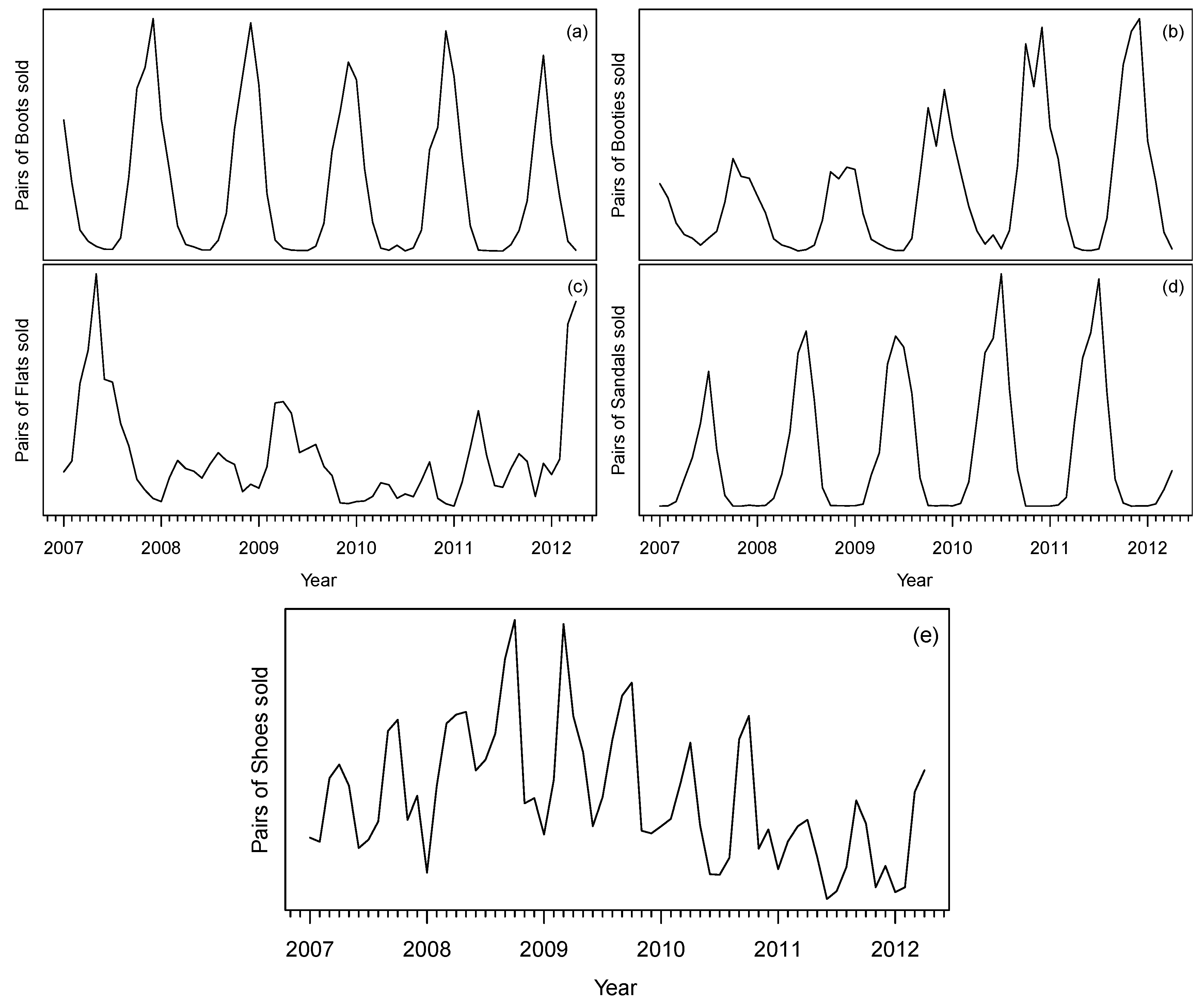
4.1. Data
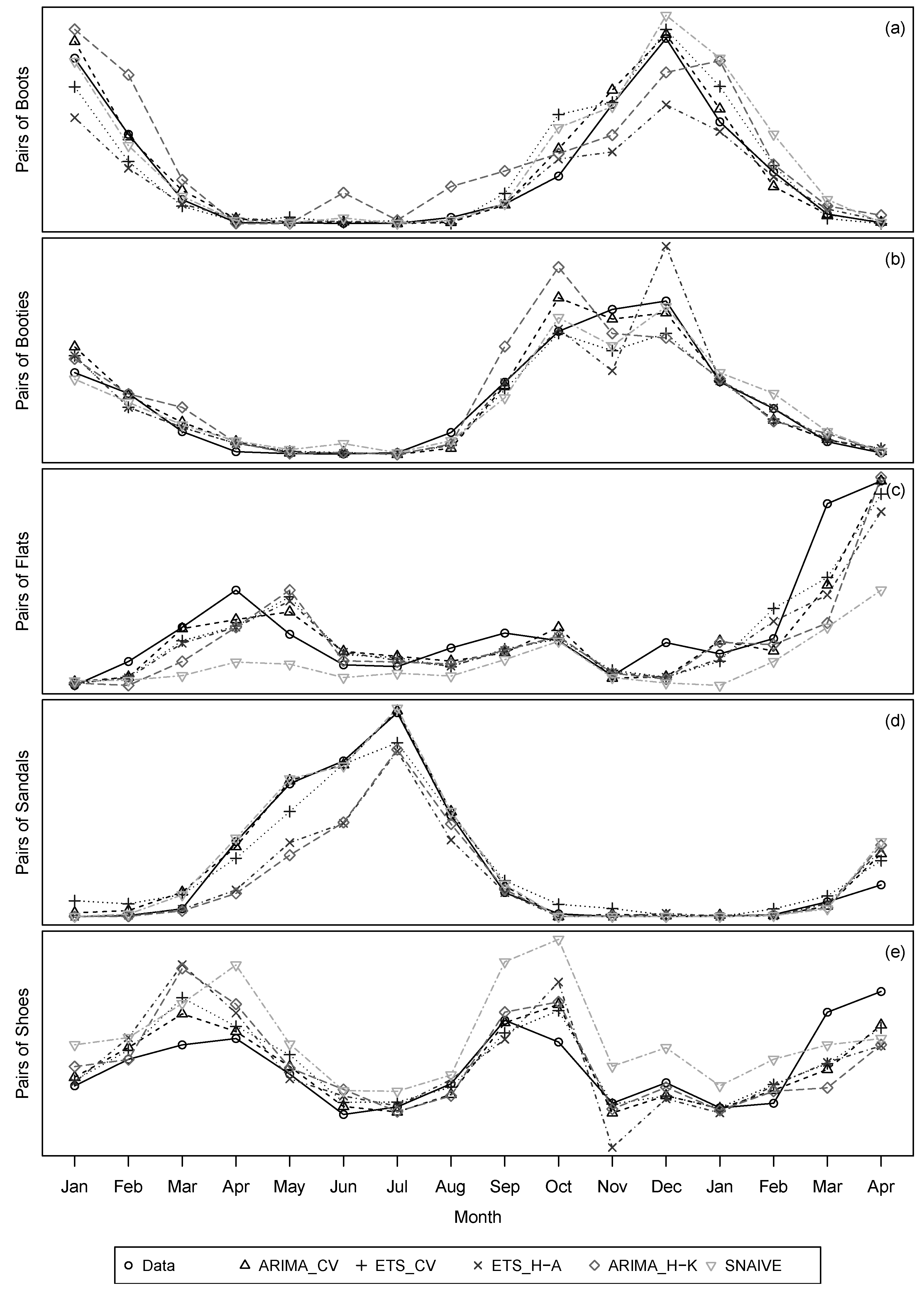
4.2. Results
5. Conclusions
Acknowledgments
Author Contributions
Conflicts of Interest
References
- Alon, I. Forecasting aggregate retail sales: The Winters’ model revisited. In Proceedings of the 1997 Midwest Decision Science Institute Annual Conference, Indianapolis, IN, USA, 24–26 April 1997; pp. 234–236.
- Alon, I.; Min, Q.; Sadowski, R.J. Forecasting aggregate retail sales: A comparison of artificial neural networks and traditional method. J. Retail. Consum. Serv. 2001, 8, 147–156. [Google Scholar] [CrossRef]
- Frank, C.; Garg, A.; Sztandera, L.; Raheja, A. Forecasting women’s apparel sales using mathematical modeling. Int. J. Cloth. Sci. Technol. 2003, 15, 107–125. [Google Scholar] [CrossRef]
- Chu, C.W.; Zhang, P.G.Q. A comparative study of linear and nonlinear models for aggregate retail sales forecasting. Int. J. Prod. Econ. 2003, 86, 217–231. [Google Scholar] [CrossRef]
- Aburto, L.; Weber, R. Improved supply chain management based on hybrid demand forecasts. Appl. Soft Comput. 2007, 7, 126–144. [Google Scholar] [CrossRef]
- Zhang, G.; Qi, M. Neural network forecasting for seasonal and trend time series. Eur. J. Oper. Res. 2005, 160, 501–514. [Google Scholar] [CrossRef]
- Kuvulmaz, J.; Usanmaz, S.; Engin, S.N. Time-series forecasting by means of linear and nonlinear models. In Advances in Artificial Intelligence; Springer: Berlin/Heidelberg, Germany, 2005. [Google Scholar]
- Box, G.; Jenkins, G.; Reinsel, G. Time Series Analysis, 4th ed.; Wiley: Hoboken, NJ, USA, 2008. [Google Scholar]
- Hyndman, R.J.; Koehler, A.B.; Ord, J.K.; Snyder, R.D. Forecasting with Exponential Smoothing: The State Space Approach; Springer: Berlin, Germany, 2008. [Google Scholar]
- Pena, D.; Tiao, G.C.; Tsay, R.S. A Course in Time Series Analysis; John Wiley & Sons: New York, NY, USA, 2001. [Google Scholar]
- Zhao, X.; Xie, J.; Lau, R.S.M. Improving the supply chain performance: Use of forecasting models versus early order commitments. Int. J. Prod. Res. 2001, 39, 3923–3939. [Google Scholar] [CrossRef]
- Gardner, E.S. Exponential smoothing: The state of the art. J. Forecast. 1985, 4, 1–28. [Google Scholar] [CrossRef]
- Makridakis, S.; Wheelwright, S.; Hyndman, R. Forecasting: Methods and Applications, 3rd ed.; John Wiley & Sons: New York, NY, USA, 1998. [Google Scholar]
- Gardner, E.S. Exponential smoothing: The state of the art-Part II. Int. J. Forecast. 2006, 22, 637–666. [Google Scholar] [CrossRef]
- Aoki, M. State Space Modeling of Time Series; Springer: Berlin, Germany, 1987. [Google Scholar]
- Hyndman, R.J.; Athanasopoulos, G. Forecasting: Principles and Practice; OTexts: Melbourne, Australia, 2013. [Google Scholar]
- Ljung, G.M.; Box, G.E.P. On a measure of lack of fit in time series models. Biometrika 1978, 65, 297–303. [Google Scholar] [CrossRef]
- Brockwell, P.J.; Davis, R.A. Introduction to Time Series and Forecasting, 2nd ed.; Springer: New York, NY, USA, 2002. [Google Scholar]
- Shumway, R.H.; Stoffer, D.S. Time Series Analysis and Its Applications: With R Examples, 3rd ed.; Springer: New York, NY, USA, 2011. [Google Scholar]
- Wei, W.S. Time Series Analysis: Univariate and Multivariate Methods, 2nd ed.; Addison Wesley: Boston, MA, USA, 2005. [Google Scholar]
- Hyndman, R.J.; Koehler, A.B. Another look at measures of forecast accuracy. Int. J. Forecast. 2006, 22, 679–688. [Google Scholar] [CrossRef]
- Arlot, S.; Alain, C. A survey of cross-validation procedures for model selection. Stat. Surv. 2010, 4, 40–79. [Google Scholar] [CrossRef]
- Hyndman, R.J.; Khandakar, Y. Automatic time series forecasting: the forecast package for R. J. Stat. Softw. 2008, 27, 1–22. [Google Scholar] [CrossRef]
- Kwiatkowski, D.; Phillips, P.C.; Schmidt, P.; Shin, Y. Testing the null hypothesis of stationariry against the alternative of a unit root. J. Econom. 1992, 54, 159–178. [Google Scholar] [CrossRef]
- R Core Team. R: A Language and Environment for Statistical Computing; R Foundation for Statistical Computing: Vienna, Austria, 2016. [Google Scholar]
- Hyndman, R.J. Forecast: Forecasting Functions for Time Series and Linear Models. R package Version 7.3. Available online: http://github.com/robjhyndman/forecast (accessed on 7 November 2016).
- Fildes, R.A.; Goodwin, P. Against your better judgment? How organizations can improve their use of management judgment in forecasting. Interfaces 2007, 37, 570–576. [Google Scholar] [CrossRef] [Green Version]


| Time Series | Model | RMSE | Rank | MAE | Rank | MAPE (%) | Rank | MASE | Rank | L-B Test |
|---|---|---|---|---|---|---|---|---|---|---|
| Boots | Log ARIMA | 736.37 | 1 | 500.67 | 1 | 90.33 | 1 | 0.60 | 1 | 0.63 |
| ETS | 1470.95 | 2 | 921.14 | 2 | 206.71 | 4 | 1.11 | 2 | 0.05 | |
| ETS Hyndman-Athanasopoulos (2013) framework | 1918.63 | 4 | 1156.32 | 4 | 138.49 | 2 | 1.39 | 4 | 0.10 | |
| ARIMA Hyndman-Khandakar (2008) algorithm | 2104.56 | 5 | 1668.49 | 5 | 978.05 | 5 | 2.00 | 5 | 0.80 | |
| Seasonal naïve method | 1649.37 | 3 | 963.75 | 3 | 179.73 | 3 | 1.16 | 3 | 0.69 | |
| Booties | Log ARIMA | 406.53 | 1 | 284.43 | 1 | 61.54 | 1 | 0.72 | 1 | 0.66 |
| ETS | 480.83 | 3 | 319.66 | 2 | 73.25 | 4 | 0.81 | 2 | 0.10 | |
| ETS Hyndman-Athanasopoulos (2013) framework | 687.41 | 4 | 369.78 | 4 | 67.90 | 3 | 0.93 | 4 | 0.10 | |
| ARIMA Hyndman-Khandakar (2008) algorithm | 733.37 | 5 | 492.01 | 5 | 66.73 | 2 | 1.24 | 5 | 0.80 | |
| Seasonal naïve method | 409.57 | 2 | 321.44 | 3 | 149.30 | 5 | 0.81 | 2 | 0 | |
| Flats | Log ARIMA | 385.69 | 1 | 265.19 | 1 | 29.62 | 1 | 0.45 | 1 | 0.06 |
| ETS | 401.61 | 2 | 299.30 | 2 | 31.32 | 3 | 0.51 | 2 | 0.55 | |
| ETS Hyndman-Athanasopoulos (2013) framework | 450.06 | 3 | 320.84 | 3 | 31.17 | 2 | 0.55 | 3 | 0.84 | |
| ARIMA Hyndman-Khandakar (2008) algorithm | 544.25 | 4 | 341.52 | 4 | 32.94 | 4 | 0.58 | 4 | 1.00 | |
| Seasonal naïve method | 750.80 | 5 | 536.44 | 5 | 47.62 | 5 | 0.92 | 5 | 0 | |
| Sandals | ARIMA | 1021.89 | 1 | 629.08 | 1 | 2217.84 | 4 | 0.55 | 1 | 0.05 |
| ETS | 1594.30 | 3 | 1259.59 | 3 | 7798.43 | 5 | 1.09 | 3 | 0.03 | |
| ETS Hyndman-Athanasopoulos (2013) framework | 3065.38 | 4 | 1866.34 | 4 | 270.90 | 2 | 1.62 | 4 | 0.07 | |
| ARIMA Hyndman-Khandakar (2008) algorithm | 3251.93 | 5 | 1921.29 | 5 | 591.37 | 3 | 1.67 | 5 | 0.41 | |
| Seasonal naïve method | 1287.04 | 2 | 670.00 | 2 | 101.78 | 1 | 0.58 | 2 | 0.44 | |
| Shoes | Log ARIMA | 607.29 | 1 | 443.88 | 1 | 12.84 | 1 | 0.35 | 1 | 0.11 |
| Log ETS | 643.73 | 2 | 481.06 | 2 | 13.76 | 2 | 0.38 | 2 | 0.54 | |
| ETS Hyndman-Athanasopoulos (2013) framework | 975.60 | 4 | 735.49 | 4 | 21.85 | 4 | 0.59 | 4 | 0.11 | |
| ARIMA Hyndman-Khandakar (2008) algorithm | 943.62 | 3 | 657.03 | 3 | 18.66 | 3 | 0.52 | 3 | 0.04 | |
| Seasonal naïve method | 1261.16 | 5 | 1096.5 | 5 | 34.79 | 5 | 0.88 | 5 | 0 1 |
© 2016 by the authors; licensee MDPI, Basel, Switzerland. This article is an open access article distributed under the terms and conditions of the Creative Commons Attribution (CC-BY) license (http://creativecommons.org/licenses/by/4.0/).
Share and Cite
Ramos, P.; Oliveira, J.M. A Procedure for Identification of Appropriate State Space and ARIMA Models Based on Time-Series Cross-Validation. Algorithms 2016, 9, 76. https://doi.org/10.3390/a9040076
Ramos P, Oliveira JM. A Procedure for Identification of Appropriate State Space and ARIMA Models Based on Time-Series Cross-Validation. Algorithms. 2016; 9(4):76. https://doi.org/10.3390/a9040076
Chicago/Turabian StyleRamos, Patrícia, and José Manuel Oliveira. 2016. "A Procedure for Identification of Appropriate State Space and ARIMA Models Based on Time-Series Cross-Validation" Algorithms 9, no. 4: 76. https://doi.org/10.3390/a9040076