
Algorithms for Drug Sensitivity Prediction

Electrical and Computer Engineering Department, Texas Tech University, Lubbock, TX 79409, USA
*
Author to whom correspondence should be addressed.
†
These authors contributed equally to this work.
Algorithms 2016, 9(4), 77; https://doi.org/10.3390/a9040077
Submission received: 31 August 2016
/
Revised: 14 November 2016
/
Accepted: 14 November 2016
/
Published: 17 November 2016
(This article belongs to the Special Issue Biological Networks)
Abstract
:Precision medicine entails the design of therapies that are matched for each individual patient. Thus, predictive modeling of drug responses for specific patients constitutes a significant challenge for personalized therapy. In this article, we consider a review of approaches that have been proposed to tackle the drug sensitivity prediction problem especially with respect to personalized cancer therapy. We first discuss modeling approaches that are based on genomic characterizations alone and further the discussion by including modeling techniques that integrate both genomic and functional information. A comparative analysis of the prediction performance of four representative algorithms, elastic net, random forest, kernelized Bayesian multi-task learning and deep learning, reflecting the broad classes of regularized linear, ensemble, kernelized and neural network-based models, respectively, has been included in the paper. The review also considers the challenges that need to be addressed for successful implementation of the algorithms in clinical practice.
1. Introduction
In recent years, the study of predictive modeling of drug sensitivity has received a boost due to the ever-growing interest in precision medicine and the availability of large-scale pharmacogenomics datasets. Drug sensitivity prediction is an integral part of personalized medicine that refers to therapy tailored to an individual patient, rather than a one-size-fits-all approach designed for an average patient. The idea of personalized medicine has been in existence since the time of Hippocrates in the fifth century BC, who treated patients based on their humor (bodily fluids) imbalances [1]. The humor approach held sway in personalized treatment for two millennia, but was debunked in the later part of the second millennium based on advanced understanding of human anatomy and physiology. Personalized therapy in the 20th century was primarily based on advanced visualization approaches, such as X-ray or Magnetic Resonance Imaging (MRI) scans along with multiple pathology tests. The ability to measure genomic features on an individual basis in the last two decades opened up numerous possibilities for personalized therapy. The genomic characterizations provide substantially more detailed information on a patient with a genetic disease as compared to phenotypic observations or non-molecular tests. If we are to define personalized therapy in the current era, the incorporation of genomic information in designing personalized therapy is quite certain. For instance, the U.S. Food and Drug Administration (FDA) considers personalized medicine (or precision medicine) to entail “disease prevention and treatment that takes into account differences in people’s genes, environments and lifestyles” (http://www.fda.gov/ScienceResearch/SpecialTopics/PrecisionMedicine/default.htm). Similarly, the National Cancer Institute (NCI) defines personalized medicine as “A form of medicine that uses information about a person’s genes, proteins, and environment to prevent, diagnose, and treat disease” (https://www.cancer.gov/publications/dictionaries/cancer-terms?cdrid=561717). An underlying theme of personalized medicine is the incorporation of patient’s genomic information besides other characteristics in therapeutic decisions.
This review primarily considers various algorithms that have been proposed to decipher and obtain relevant information from genomic and drug sensitivity characterization sources. These data sources are used to design models that can predict: (1) the sensitivity of a new tumor culture or cell line to an existing drug or combinations of them or (2) the sensitivity of an existing tumor culture to a new drug or to a drug combination. We should note that cell lines are the most commonly-used approach to study cancer biology and test various cancer treatments. Cell lines usually contain cells of one type and can be either genetically identical or diverse. These cell lines are easy to grow in a laboratory, and multiple research groups can have access to the same cell line for corroborating research findings and to build a body of knowledge based on a specific genetic type of cell. Cancer cell lines are expected to reflect the properties (such as genotypic and phenotypic characteristics, mutation status, gene expression and drug sensitivity) of the original cancer type from which they were cultured [2,3]. However, the laboratory environment along with the absence of other regular cell types within the cell line restricts the ability of a cell line itself to mimic in vivo cancer growth, as well as the efficacy of anti-cancer drugs [4]. On the other hand, primary tumor cultures are those established from the tumor biopsy of a patient, and they reflect the surroundings in the original sampled tissue. As compared to cell lines, primary cell cultures are more heterogeneous and also contain a small fraction of normal stromal cells, which can be an advantage since tumor response is often influenced by an interplay of the tumor cells and the non-malignant cells within the tumor microenvironment. Since different cells have diverse growth rates in culture conditions, the primary cell culture may lose its heterogeneity as in the original tumor biopsy. As time goes by, some particular cell types may grow rapidly under culture conditions, and they will become predominant. Thus, short-term drug sensitivity studies on the recently-extracted primary tumor culture can capture the heterogeneity from the patient’s tumor.
The accuracy and precision of drug sensitivity modeling is highly dependent on associated factors, like data types, feature selection, model selection and model validation. Therefore, we structured this review in a manner such that we can discuss each one of these individual steps. In terms of the models used to predict drug sensitivity, we consider models based on genomic characterization alone, along with models based on both genomic and functional characterizations.
2. Data Characterizations
A crucial preliminary step in drug sensitivity prediction analysis involves collecting information on various aspects of the biological system. The observations can involve internal genetic states of the systems, such as mutation and gene expression, or phenotypic changes following perturbations to the system, such as cell viability measurement after applying various drugs. This section will provide an overview of genomic and functional characterizations that are commonly used in drug sensitivity prediction studies. A pictorial representation of the various data types is shown in Figure 1.
Genomic characterization data can be derived from different levels of the cell, such as the genome, transcriptome, proteome or metabolome, with each level playing a specific role in the conversion of information coded in DNA to functional activities in the cell. The levels can potentially provide diverse sets of information, such as mutations in the genome or altered transcriptional behavior, that can assist in predicting the sensitivity of the tumor to a drug. For instance, a commonly-considered genetic test for breast cancer patients involves the measurement of HER2 protein expression. HER2 overexpressed patients are usually prescribed therapy with either of the targeted drugs trastuzumab, pertuzumab or lapatinib that interfere with the HER2 receptor [5,6]. However, it has been observed that not all patients with HER2 overexpression measured by immunohistochemistry show gene amplification as when measured by fluorescence in situ hybridization [7,8,9]. Thus, it is highly relevant to explore the various levels of biological activities in a cell, as sensitivity to a drug may be explained by different combinations of activities at various genomic levels.
At the DNA level, Single Nucleotide Polymorphisms (SNPs) denote variations in a single nucleotide block. As an example, an SNP may denote replacement of cytosine (C) by thymine (T) in a stretch of DNA. Copy Number Variations (CNVs) signify duplications of stretches of DNA and can denote several copies of a gene. SNPs and CNVs are biomarkers that play an important role in analyzing the response to drugs, as an over-amplification of some genes as captured by CNV measurements can represent the activation of oncogenes. As an example, a higher copy number of the EGFR gene has been observed for some non-small-cell lung cancer patients, and the information can be used to predict sensitivity to the targeted EGFR inhibitor drug gefitinib [10]. Similarly, deletions or mutations in tumor suppressor genes, as captured by CNV or SNP measurements, may lead to loss of function resulting in tumor growth.
At the epigenetic level, DNA methylation is the process of methyl groups attaching to DNA that can alter the transcription process. A form of aberrant DNA methylation observed in cancer involves inactivation of tumor suppressor genes by hyper-methylation of the large CpG dinucleotide clusters located in their promoter islands [11]. These aberrations are often targeted by DNA-demethylating agents [12,13].
At the transcriptomic level, RNA expression is measured by various profiling techniques, such as microarray [14], SAGE [15], MPSS [16] and RNA-Seq [17], and each technology has its own benefits and concerns. A common example of gene expression application to guide cancer therapy includes the usage of trastuzumab for the overexpression of HER2 (ERBB2) in breast cancer patients.
It is quite often the case that observations from the proteomic level using technologies, such as the 2D gel electrophoresis technique (2D-GE) [18], MALDI imaging mass spectrometry [19] or reverse-phase protein array [20], are also considered for anti-cancer therapeutic decision making.
Another level of information observed through metabolites [21] is currently being considered to provide unique insights on the potential sensitivity of drugs, as the metabolism of cancerous cells is quite different from normal cells.
A number of separate large-scale experimental studies have been conducted on cancer cell lines or patient tumor cultures to observe the effect of applied drugs and results subsequently published as pharmacogenomics databases. NCI60 [22] has applied CDNA microarrays to observe the variation among 8000 genes in 60 cell lines for anti-cancer drugs and provides DNA copy number variation, mutation and protein expression information. In the Cancer Cell Line Encyclopedia (CCLE) [23] database, gene expression and Single Nucleotide Polymorphism (SNP6) expressions are included for about and genes respectively, for 947 human cancer cell lines, along with sensitivities for 24 drugs. While in the Cancer Genome Project (CGP) [24], 75,000 experiments have been conducted to generate the response of 138 anti-cancer drugs across >700 cancer cell lines and gene expression, mutation and CNV information for >23,000 genes. Additionally, a collaborative NCI and the Dialogue on Reverse Engineering Assessment and Methods (DREAM) initiative [25] to predict drug response based on a group of genomic, epi-genomic and proteomic profiling datasets provided six characterizations (gene expression, methylation, RNA sequencing, exome sequencing, Reverse Phase Protein Array (RPPA) and SNP6) for 53 breast cancer cell lines and 35 anti-cancer drugs. The Cancer Genome Atlas (TCGA) [26] has profiled and analyzed large numbers of human patient tumors to find the molecular aberrations among genes with proteomic and epigenetic expression. The dataset includes a total of 5074 tumor samples, out of which 93% has been assessed for RPPA, DNA methylation, copy number, mutation, microRNA and gene expression, but they are yet to include drug sensitivity for anti-cancer drugs. Responses of 70 breast cancer cell lines to 90 experimental or approved therapeutic agents have been reported in the GRAY database [27]. The dataset includes characterizations of copy number aberrations, mutations, gene and isoform expression, promoter methylation and protein expression. The Genentech (GNE) database [28] describes RNA sequencing and SNP array analysis of 675 human cancer cell lines along with responses to a PI3K inhibitor (GDC-0941) and a MEK inhibitor (GDC-0973). While in the Personal Genome Project (PGP) database [29], the PF-03814735 inhibitor of Aurora kinases was tested in vitro in a panel of 87 cancer lines derived from human lung, breast and colorectal tumors, where characterizations of mutation and gene expression data were determined. The Cancer Therapeutics Response Portal (CTRP) [30] contains the response of 860 deeply-characterized cancer cell lines to 481 small-molecule probes that target specific nodes of important cellular processes.
The preceding description considered various genomic characterizations of a tumor cell line or culture, and we next discuss various approaches to measure the response of tumors to various drugs. The drug responses are usually observed using pharmacological assays that measure metabolic activity in terms of reductase-enzyme product or energy-transfer molecule ATP levels following 72–84 h of drug delivery. The cell viability drug screenings are usually conducted using a robotic system where drugs are delivered to small wells containing a portion of the cell culture of interest. Examples of such commercial sellers include GNF Systems (http://gnfsystems.com) and Wako Automation (http://www.wakoautomation.com).
Each well is expected to contain more than 100 cells. Experiments are conducted with multiple drug concentrations (around 5–10 concentrations), and the luminescence in each well is measured at the steady state to assess cell viability. A dose response curve for each cell line and a specific drug is generated by observing the cell viability at different drug concentrations to fit a curve through the observations as shown in Figure 2. A dose-response curve is often approximated by a sigmoidal, linear or a semi-log curve. An example of sigmoidal curve generation is shown in Equation (1) [23].
where and represent the minimum and maximum reduction in cell viability, represents the drug concentration required to reach 50% of (average of the minimum and maximum cell viability attainable by the drug) and h is the Hill slope. Rather than using the entire cell response curve as the measure of sensitivity, a specific feature of the curve such as AUC (Area Under the dose response Curve) or (drug concentration required to reduce cell viability to 50% of initial response) is used to represent sensitivity. The IC’s are usually converted to sensitivity values between zero and one using a logarithmic mapping function, such as [31,32].
Each feature of the dose response curve can produce its own set of concerns. For instance, for responses where 50% cell viability cannot be reached, is often equated to , which does not capture the exact behavior of the dose response curve. AUC can be problematic when low doses are used and an initial increase in cell viability is observed, which will result in negative portions for the AUC.
3. Feature Selection
A significant number of current drug sensitivity studies use high throughput technologies to collect information from various genomic levels resulting in extremely high dimensional genomic characterization datasets. For instance, the Cancer Cell Line Encyclopedia study [23] has >50,000 features representing mRNA expressions and mutational status of thousands of genes. Since only a small set of these features is important for drug sensitivity prediction and the number of samples for training is significantly less than the number of available features, direct application of machine learning tools on all of these features can result in model overfitting. Figure 3 shows an example trajectory for training error and generalization error with the increase in the number of features. The synthetic example was created with 100 random samples of 90 features each where the output response is dependent only on the first 10 features. The true error was estimated based on the additional holdout of 300 samples with the model trained using 100 samples. This example with synthetic data was created to illustrate the effect of overfitting with increased model complexity. Figure 3 shows the average behavior over 100 random simulations. Since our output response is only dependent on the first 10 features, we note that the validation error keeps increasing when the number of features is increased beyond 10. After a point, the addition of more features in modeling can be detrimental from the prediction accuracy perspective. If the model complexity (in this case, represented by the number of features) is high relative to the number of training samples, the estimated model can fit the training data precisely, but can produce a large error when predicting unseen data (generalization error). Note that in drug sensitivity studies, the number of features is usually significantly higher (in the range of –) as compared to the number of samples (in the range of 60–1000), and thus, overfitting is a highly pertinent problem.
The issue of overfitting can be addressed in various ways. We will broadly categorize them as follows:
- Filter feature selection: Feature selection refers to selecting a subset of features from the full set of input features based on some design criteria. In filter feature selection, the features are be rated based on general characteristics, such as statistical independence or the correlation of individual features with output response. Some commonly-used filter feature selection approaches in drug sensitivity prediction include: (i) correlation coefficients between genomic features and output responses [25]; (ii) ReliefF [33,34], which is computationally inexpensive, robust and noise tolerant, but does not discriminate between redundant features; (iii) minimum Redundancy Maximum Relevance (mRMR) [35,36,37], which considers features that have highly statistical dependencies with output response, while minimizing the redundancy among selected features.
- Wrapper feature selection: Wrapper techniques evaluate feature subsets based on their predictive accuracy based on a particular model. As compared to wrapper approaches, filter feature selection methods are computationally inexpensive, but they tend to introduce bias and sometimes miss the multivariate relationships among features. A feature may not perform well individually, but in combination with other features, can generate a highly accurate model. Computationally-intensive wrapper methods tend to capture the feature combinations with higher model accuracy, but can potentially overfit the data as compared to filter approaches. In wrapper methods, the goodness of a particular feature subset for feature selection is evaluated using an objective function, , which can model accuracy measured in terms of mean absolute error, root mean square error or the correlation coefficient between predicted and experimental responses. Some commonly-used wrapper feature selection approaches in drug sensitivity prediction include: (i) Sequential Floating Forward Search (SFFS) [32,38], where at each forward iteration, the feature from the remaining features that maximizes the reward or minimizes the cost is selected, and the floating part provides the option to remove an already selected feature if it improves the objective function; (ii) recursive feature elimination [39], which initially involves the ranking of features based on a model fit to all features and recursively eliminating the lowest ranked ones.
- Embedded feature selection: As compared to wrapper feature selection approaches that are evaluated based on objective functions without incorporating the specific structure of the model, embedded feature selection approaches consider the specific structure of the model to select the relevant features, and thus, the feature selection and learning parts cannot be separated. A commonly-used embedded approach is regularization that penalizes the norms of feature weights, such as ridge regression [40,41] penalizing the norm, LASSO [42,43] penalizing the norm and elastic net regularization [23,44] penalizing a mix of and norms.
- Feature extraction: Dimensionality reduction can be approached based on feature extraction from the input data where input data vectors are mapped to new coordinates using different functions. One common example of feature extraction approach is Principal Component Analysis (PCA) [45,46], which maps the input data to a coordinate system that is orthogonal to each other and with the property that the variance along each component projection is maximized.
- Biological knowledge-based feature selection: This approach is based on using prior biological knowledge to reduce the size of the relevant feature set. For instance, if the drugs considered are kinase inhibitors, a potential approach to feature selection might involve modeling from a set of around 500 available kinases [47,48]. Other approaches can include incorporating pathway knowledge in data-driven feature selection, such as pathway-based elastic net regularization [49], biological pathway-based feature selection integrating signalizing and regulatory pathways with gene expression data to select significant features that are minimally redundant [50] or the use of the activation status of signaling pathways as features [51].
4. Predictive Models
Models capable of predicting the response of a tumor culture to a new drug (or drug combination) or the response of a new tumor culture to a commonly-used drug can be estimated from genomic, or functional characterizations, or a combination of both. We will first discuss techniques that are commonly used to estimate predictive models from genomic characterizations followed by predictive models designed from a combination of genomic and functional characterizations. The predictive models designed from genomic characterizations alone tend to predict the response of a new tumor culture or cell line to an existing drug that has been tested on a range of cell lines.
A variety of methodologies has been proposed for drug sensitivity prediction based on genomic characterizations. The typical practice is to consider a training set of cell lines with experimentally-measured genomic characterizations (such as RNA-Seq, microarray, protein RPPA, methylation, SNPs, etc.) and responses to different drugs, to design supervised predictive models for each individual drug based on one or more genomic characterizations. The proposed modeling techniques have been diverse, involving commonly-used traditional regression approaches, such as linear regression with regularization or problem-specific new developments that incorporate prior biological knowledge of pathways. The majority of developments have considered steady state models due to the limited availability of time-series data following drug applications. The performance of a similar class of models can differ considerably based on the type of data pre-processing, feature selection, data integration and model parameter selection applied during the design process. Some of the key challenges of drug sensitivity model inference and analysis include (a) the extreme large dimension of features as compared to the number of samples; (b) limited model accuracy and precision; (c) data generation and noise measurement and (d) lack of interpretability of models in terms of the biological relevance of selected features.
A recent study on the performance of modeling frameworks [52] using large-scale pharmacogenomics screen data considered over 110,000 different models based on a multifactorial experimental design evaluating systematic combinations of modeling factors, such as (i) the type of predictive algorithm; (ii) the type of molecular features; (iii) the kind of drug whose sensitivity is being predicted; (iv) the method of summarizing compound sensitivity values and (v) the type of sensitivity response whether discrete or continuous. Results from the systematic evaluation suggest that the model input data, specifically the type of genomic characterizations and choice of drug, are the primary factors explaining modeling framework performance, followed by the choice of algorithm. In this study, the choices of modeling algorithms that showed the best performance were ridge regression and elastic net. We next discuss the linear regression models to provide an overview of ridge regression and elastic net.
4.1. Linear Regression Models
In a predictive modeling setting, linear regression is one of the most commonly-applied models. Linear regression has been extensively studied and with it the statistical properties of the parameter estimation for linear models, which are easier to determine as compared to the non-linear scenario.
To explain a linear model, consider and ( to denote the training predictor features and output response samples, respectively. A linear regression model considers the generation of regression coefficients , such that is minimized. The minimization of the error term is usually considered in the sum of squared error sense, i.e., minimize . For linear regression, we generally incorporate a constant term commonly known as the intercept, i.e., . In terms of matrix notation, we can write it as follows:
The vector consists of the response or dependent variables; consists of the regressors, predictor or independent variables; vector β is the parameter vector that needs to be estimated; and ϵ denotes the error or disturbance terms.
Note that the development of the linear regression framework consists of a linear combination of parameters and predictor variables. Transforming the predictor variables to higher orders can allow us to utilize the framework in modeling with nonlinear terms, which is known as polynomial regression [53].
Ordinary least squares is the simplest form of linear regression where our goal is to select β, such that it minimizes . Ordinary least squares-based linear regression models are straightforward to understand and relatively simple to interpret in terms of feature weights and their positive or negative influences. However, it is not suitable to solve the large feature dimension problem with limited samples, and overfitting is a common problem. Some of the assumptions of ordinary least squares are not satisfied in drug sensitivity studies, such as output response being a linear summation of covariates, and thus, ordinary least squares is not the best approach in terms of predictive accuracy. Thus, ordinary least squares are suitable for scenarios where the number of features has already been reduced to a smaller set, and we are interested in an easily interpretable and robust model rather than a highly accurate one. A commonly-used modification to ordinary least squares is to add a regularization term in the cost function to avoid overfitting. Regularization usually consists of adding a penalty on the complexity of the model, which in regression is often included in the form of or norms added to the cost function . When the additional penalty term consists of the square of the norm of β, it is known as ridge regression [54]:
is a tuning parameter that provides a control on fitting a linear model and shrinking the parameter coefficients. When the penalty term consists of the norm of the parameter vector, it is known as Least Absolute Selection and Shrinkage Operator (LASSO):
LASSO [44] has shown to provide good performance and feature selection properties, but also suffers from the following limitations: (a) when n is smaller than M, LASSO selects at most n features before it saturates; and (b) LASSO usually selects one variable from a group of highly correlated variables, ignoring the others.
To avoid the limitations of LASSO, elastic net combines the penalties of ridge regression and LASSO to arrive at:
It has been shown that the elastic net regression can be formulated as a support vector machine problem, and resources applied to support vector machine solutions can be applied to elastic net, as well [55].
The initial publication on the Cancer Cell Line Encyclopedia [23] considered elastic net as the model for predicting drug sensitivity based on over 100,000 genomic features. For molecular features, the authors considered an integrated set of gene expression, gene copy number, gene mutation values, lineage, pathway activity scores derived from gene expression data and regions of recurrent copy number gain or loss derived from the Genomic Identification of Significant Targets in Cancer (GISTIC) [56].
Ridge regression has been used in [57] to predict chemotherapeutic response in patients using only before-treatment baseline tumor gene expression data. The authors compared the performance with other approaches like random forests [58], nearest shrunken centroids [59], principal component regression [60,61], LASSO [42] and elastic net [44] regression and observed that ridge regression was the best performer. However, other studies comparing multiple algorithms on a drug sensitivity database [25] have observed that random forests or kernelized Bayesian multitask learning [62] perform better than ridge regression or other regularized linear regression approaches. As mentioned earlier, both the drug type that is being predicted or the different molecular features being used to design the predictive model can play a significant role. For instance, in the study [57], they used chemotherapeutic, whereas [25] used primarily targeted drugs. Furthermore, [57] used gene expression data alone, whereas [25] used multiple types of genomic data, including gene expression, RNA-Seq, RPPA, methylation, CNV and SNP.
We next attempt to provide an overview of the other modeling algorithms that are commonly used for comparing the performance of drug sensitivity predictive models.
4.2. Logistic Regression and Principal Component Regression-Based Techniques
Logistic regression refers to a regression model where the response or dependent variable is categorical [63,64]. The model estimates the probability of the categorical dependent variable based on the predictor variables using the logistic function: . To explain logistic regression, consider a binary outcome Y, and we want to model . The logistic regression model based on logit transformation of the probability and subsequently equating it to a linear combination of predictors will consist of:
where can be computed as:
Logistic regression has been used as one of the comparison methods for drug sensitivity prediction in multiple studies [25,65,66,67].
Principal Component Regression (PCR), as the name suggests, is based on principal component analysis. The principal components of the dependent matrix are calculated, and the regression of on is fitted using ordinary least squares. The regression coefficients in the transformed space are mapped back to the original space to arrive at the principal component regression coefficients. The primary difference with ordinary least squares is that the regression coefficients are computed based on the principal components of the data. When a subset of the principal components is used for generating the regression coefficients, it acts similar to a regularization process. Principal component regression can also overcome the problem of multicollinearity in ordinary least squares [60].
Principal component regression has been used as one of the comparison methods for drug sensitivity prediction in multiple studies, as well [25,52,57].
Partial Least Squares (PLS) regression [68] has similarities to principal component regression, but projects both and to new spaces before generating the regression model. The intent is that the model might have few underlying factors that are important, and using these latent factors in prediction can avoid overfitting [69]. Similar to PCR, PLS is often used as a comparison method in multiple drug sensitivity prediction studies [25,39,52]
PCR and PLS utilize derived input directions and select a subset of the derived directions for modeling. PCR keeps the high variance directions and discards the low variance ones, whereas PLS also tends to shrink the low variance directions, but can inflate the high variance regions [70]. Both PCR and PLS have similarities with ridge regression that shrink in all directions and more so in low variance directions. In terms of predictive performance, ridge regression is usually preferable over PLS and PCR [71].
4.3. Kernel Based Methods
The most commonly-used kernel-based method for regression modeling consists of support vector regression. Support vector regression is based on the statistical learning theory or Vapnik–Chervonenkis (VC) theory developed by Vladimir Vapnik and Alexey Chervonenkis during the 1960s [72,73,74]. VC theory attempts to provide the statistical underpinnings of learning algorithms and their generalization abilities. Support Vector (SV) classifiers and subsequently SV regression showed high accuracy in comparison to existing approaches and became a commonly-used tool in classification and regression modeling [75,76,77,78].
To explain SV regression, consider and ( to denote the training predictor features and output response samples, respectively. In terms of SV regression, the goal is to find a function that has at most deviation ϵ from actual values [77], and a characteristic of the function is minimized. Thus, the deviation of the function approximator f from the actual values is being limited while minimizing some characteristic of the approximator. For explanation purposes, consider the following linear function:
Here, the function characteristic will be the norm of w. The problem can be posed as an optimization problem as follows:
To extend the SV algorithm to the nonlinear scenario, kernels are usually employed. Some commonly-used kernels are [77]:
- homogenous polynomial kernels k with and:
- inhomogenous polynomial kernels k with , and:
- radial basis kernels:
Support vector machines can handle non-linearity based on the use of kernels and tend to have better predictive performance compared to regularized regression approaches [79]. However, the direct biological interpretability of the generated model is limited. Support vector machines strike a balance on generalization error performance and can handle various noise models. For further details on SV regression models, readers are referred to a tutorial on SVMs by Smola and Schölkopf [77].
Support vector regression has been used for drug sensitivity prediction on the Cancer Cell Line Encyclopedia database in [39] using baseline gene expression as features. Other studies involving support vector regression for drug sensitivity prediction include [25,52,66]. The work in [52] considers a comparative study of multiple machine learning algorithms, including support vector regression for drug sensitivity prediction on CCLE and Sanger datasets. In their analysis, ridge regression and elastic net outperformed support sector regression. However, the likely reason for this behavior is the inbuilt embedded feature selection inherent in ridge regression and elastic net as compared to support vector regression.
4.4. Ensemble Methods
This section discusses various approaches that integrate predictions from multiple models to arrive at the final prediction. The combination can consist of picking one model out of multiple regression models based on cross-validation error or a function of the individual regression predictions.
Boosting attempts to arrive at a strong learning algorithm by combining an ensemble of weak learners. The most popular form, AdaBoost (adaptive boosting), was developed to combine weak classifiers to arrive at a high accuracy classifier [80], where later, weak classifiers are adaptively designed to correctly classify harder to classify samples.
Bootstrap aggregating (or bagging) was introduced by [81] to improve classification accuracy by combining classifiers trained on randomly-generated training sets. As the name suggests, the training sets are generated using the bootstrap approach or, in other words, generating sets of n samples with replacement from the original training set. A specified number of such training sets is generated, and the responses of models trained on these training sets are then averaged to arrive at the bagging response.
Stacked generalization (stacking) [82,83] is based on training a learning algorithm on individual model predictions. One common approach is to use a linear regression model to then combine these individual model predictions [84].
Random forest regression [58] has become a commonly-used tool in multiple prediction scenarios [25,48,85,86,87,88,89,90,91,92] due to its high accuracy and ability to handle large features with small samples. Random forest [58] combines the two concepts of bagging and random selection of features [93,94,95] by generating a set of T regression trees where the training set for each tree is selected using bootstrap sampling from the original sample set, and the features considered for partitioning at each node are a random subset of the original set of features. Regression tree is a form of non-linear regression model where samples are partitioned at each node of a binary tree based on the value of one selected input feature [96]. The bootstrap sampling for each regression tree generation and the random selection of features considered for partitioning at each node reduces the correlation between the generated regression trees, and thus, by averaging their prediction responses, it is expected to reduce the variance of the error.
Random forests tend to have high accuracy prediction and can handle a large number of features due to the embedded feature selection in the model generation process. Note that when the number of features is large, it is preferable to use a higher number of regression trees. Random forests are sufficiently robust to noise, but the biological interpretability of random forests is limited. Random forest was one of the top performing algorithms in the NCI-DREAM drug sensitivity prediction challenge [25,48], and it has been used in multiple other drug sensitivity studies [34,66,85,97]. Improvements to random forests in terms of incorporating multi-task learning that utilizes the relationships between output drug responses has been considered in [34]. The work in [34] considers a copula-based regression tree node cost function to design multivariate random forests that are shown to perform better than regular random forests when the drugs are related.
4.5. Deep Neural Networks
In this section, we consider the broad class of deep neural network-based algorithms that have recently been applied for predictive modeling tasks in chemoinformatics, which is closely related to the field of drug sensitivity prediction. As part of the molecular diversity analysis in chemoinformatics, we find the Quantitative Structure Activity Relationship (QSAR) as a popular methodology that intends to model the relationship of the chemical and physical properties of compounds with their chemical structure. All of these elements can be summarized as the pharmacokinetics properties of the compound: potency, absorption, distribution, metabolism, elimination and toxicity. Other than using the previously-described approaches of regularized linear regression, ensemble models and kernel-based models in QSAR modeling, Deep Neural Networks (DNN) is also being applied. DNN is starting to gain popularity since there have been methodology improvements that allow model training using smaller datasets with minor overfitting using weight penalties, early stopping criteria or new approaches, such as random dropout [98] and unsupervised complementary priors with stochastic binary communication [99]. The hidden layers inside the DNN models can additionally make use of the chain rule structure (shown in Figure 4) and Stochastic Gradient Descent (SGD) [100] to map the input feature to another domain where there is less redundancy and features are more orthogonal to each other. This characteristic creates sparsity training that can boost the performance of the DNN model.
Similar to the DREAM challenge for drug sensitivity prediction, Merck organized the Molecular Activity Challenge (https://www.kaggle.com/c/MerckActivity) where the purpose is to analyze independent datasets and predict which molecules will have higher activity towards their desirable biological targets and avoid targets that may result in harmful or undesirable side effects. The 2012 winners of the challenge [101] used multi-task learning for QSAR in conjunction with several neural network-based models, improving Merck’s internal criterion by 15%.
4.6. Integrated Functional and Genomic Characterization-Based Models
The predictive modeling approaches based on genomic characterizations alone are often restricted in their accuracy as the genomic characterizations observed under normal growth conditions can only provide a single snapshot of the biological system. The model inferred from analyzing multiple samples is primarily an aggregate model with the expectation that new tumor samples will activate distinct parts of the model, which will be sufficient to distinguish their diverse responses to drugs. This methodology will provide reliable results when the tumor samples have limited variations in their pathways and the tumor type is well characterized. However, for less studied tumors like sarcoma and tumors exhibiting numerous aberrations in the molecular pathways, it is desirable to investigate further the personalized inference of pathway structure. Perturbing the patient tumor culture using various known disturbances in the form of targeted drugs and observing the responses can be utilized as additional information to gain further insights on the specific patient tumor circuit. Based on this idea, a computational modeling framework to infer target inhibition maps utilizing responses of a tumor culture to a range of targeted drugs was considered in [32,47]. The target inhibition profiles of the drugs and the functional responses are utilized to infer potential tumor proliferation circuits that can assist in the generation of synergistic drug combinations.
The previously-described drug sensitivity prediction approaches are primarily based on genetic and epigenetic characterizations alone without the incorporation of drug target profiles. As an alternative perspective, rather than designing a model based on the response of a single drug to multiple different genetic samples, the response of one genetic sample to multiple different drugs is considered. The multiple drugs are applied through a drug screen with known target inhibition profiles, and their steady state response allows us to create the target inhibition map, which can predict the sensitivity to any combination of target inhibitions. The drugs included in the drug screen are often kinase inhibitors, and thus, the starting number of targets is limited to around 500 kinases of the human kinome.
The difference in the datasets used in this approach as compared to earlier approaches can be illustrated through Figure 1, which shows the details of the various datasets used for generating drug sensitivity models. G denotes the matrix of genetic characterizations of size , where number of cell lines or tumor cultures and the total number of genomic features. R denotes the drug response matrix of size in some form of characteristics of the drug response curves (such as , area under the curve, etc.), where the number of drugs. K denotes the drug target profile matrix of size where L denotes the total number of drug features. The currently-available prediction approaches based on genetic characterizations primarily consider the matrix G and a column of R to generate a model that can predict the response to that drug for a new genomic characterization. The integrated approach considers K and a row of R, along with the corresponding row of G to generate a predictive model that can predict the response to a new drug or drug combination with known target inhibition profiles.
To decipher a predictive model from K, R and G, a number of biological constraints were considered in [32,47]. The objective elements of molecularly-targeted drugs [102,103,104,105,106] are primarily oncogenes (genes with potential to cause tumor proliferation while getting stuck in a constant activation state), and thus, increased inhibition of an oncogene is expected to increase the sensitivity (reduce cell viability). This prior biological knowledge can be incorporated as constraints in the framework. For two drugs and , the biologically-motivated constraints can be described as:
- C1: If , then
- C2: If , then
Once the set is generated for the cell culture, the goal is to generate the prediction where denotes the target pattern for a new drug or drug combination. A search for the set of subset drugs from the training set that satisfies for is performed. Similarly, a search for the set of superset drugs from the training set that satisfies for is executed. Based on the biological constraints C1 and C2, the sensitivity can be assumed to satisfy the following inequality:
Subsequent enhancements to the modeling framework constituted (a) integration of genetic information in the prediction framework to remove false positive targets [31]. The integrated model incorporating functional and genomic information was shown to outperform multiple predictive techniques (elastic net, random forests) based on genetic characterizations when tested on publicly-available cancer cell line sensitivity databases [31]; (b) Algorithms to estimate the possible dynamic models representing a given static target inhibition map were designed in [108,109] along with optimized protein expression measurements following the application of target inhibitions to identify the specific dynamic model; (c) Quantifying the predictive power of a drug screen was considered in [110], and optimized selection of combination drugs based on set cover and the hill climbing approach was considered in [111]; (d) Validation of the prediction efficacy of in vitro single agent and combination drugs in patient-derived Diffuse Intrinsic Pontine Glioma (DIPG) primary cell cultures and cell lines was shown in [112]; (e) Validation of the sensitivity prediction of individual drugs based on in vitro canine osteosarcoma primary cell cultures (<10% 10-fold cross validation error for four tumor cultures) was reported in [31,32]).
Rather than using drug targets as they were utilized for the target inhibition map framework, the chemical descriptors of a drug can also be considered for designing an integrated model. For instance, [113] considered the design of machine learning models (neural networks and random forests) for drug sensitivity prediction that utilized both genomic characterizations and chemical descriptors as input features. The work in [114] considers the design of decision trees, support vector machines, random forests and rotation forests [115] for anti-cancer drug response prediction from both genomic characterizations and chemical descriptors. The rotation forest technique applies PCA to K subsets of the feature set to generate K separate trees from the extracted features for creating an ensemble. The study produced better results than regular random forests, and the robustness of its performance is claimed to be due to the rotation of the feature space resulting in diverse individual trees while maintaining accuracy.
4.7. Prediction Performance
This section considers a predictive performance comparison between different genetic characterization based models for the CCLE dataset. We have selected the methodologies of Elastic Net (EN), Kernelized Bayesian Multitask Learning (KBMTL), Random Forest (RF) and Deep Neural Network (DNN) as the representative methodologies for the four broad categories of regularized linear regression, kernel-based modeling, ensemble methods and deep learning, respectively.
For EN tuning of parameters α and λ, we have followed the approach in the original CCLE paper that considered elastic net for predictive modeling of drug sensitivity [23]. The optimal choice of the two parameters is selected to minimize root mean squared error for 10-fold cross-validation of training data, where 10 random values of α∈ [0.2,1] and 250 random values of are used for optimization.
For RF generation, we have used 200 trees for the forest, 10 random features for each split decision and 5 minimum entries in leaf nodes similar to the parameters considered in [34]. We have implemented KBMTL using the algorithmic code provided in [62]. Based on the parameters used in [62], we have considered 200 iterations and gamma prior values (both α and β) of one. Subspace dimensionality has been considered to be 20, and the standard deviation of hidden representations and weight parameters are selected to be the defaults and one, respectively.
For DNN, we have used a fully-connected structure that has one hidden layer:
where y is the output layer, and are the weight and bias matrix for output layer and and are weight and bias matrix for hidden layer and σ is the activation function. In our model, we use a Rectified Linear Unit (ReLU) function as our activation function. The input layer’s dimension is 200; the output layer’s dimension is one; while the hidden layer has 100 neurons. During the training, a mini-batch based SGD is used [116]. The mini-batch size is five, and the learning rate is 0.0001. In order to prevent curvature issues [117], a 0.9 momentum is added to the SGD. The whole training stops at 1000 epochs.
Table 1 shows the predictive performance in the form of correlation coefficients between actual and predicted drug sensitivity (AUC) for EN, KBMTL, RF and DNN for four drugs in the CCLE dataset [23]. We consider hold-out error estimation where 350 samples have been used as training, and the remaining samples (in the range of 140) are used for testing. Feature selection using ReliefF [33] has been used to reduce the number of gene expression features from 18,988 to 200. We observe that RF produces the best performance followed by KBMTL, EN and DNN. The worst performance of DNN is likely due to the limited number of samples used for training the model. DNN is preferable for scenarios where the number of samples is significantly higher than the number of features.
5. Biological Analysis
The standard procedure used to compare drug sensitivity prediction algorithms consists of evaluating a fitness measure, such as a difference measure of a norm between experimental responses and predicted values or a similarity measure of the correlation coefficient between the vector of predicted and actual experimentally-derived sensitivities. Relative measurements, such as the Akaike Information Criterion (AIC) [118], Bayesian Information Criterion (BIC) [70], minimum description length [119] and Vapnik–Chervonenkis (VC) dimension [74], are also occasionally considered [67,120,121]. The sample selection approaches commonly considered in drug sensitivity predictive model evaluation involve techniques, such as k-fold cross-validation [32], bootstrap [48] or hold-out [25].
Other than evaluating the performance of a generated model using existing drug sensitivity data based on techniques discussed in the previous paragraph, new experiments can be conducted to validate hypotheses generated from the estimated models. For instance, [112] used in vitro DIPG cancer cell lines to validate model hypotheses of synergistic drug pairs. The commonly-used experimental approaches included the use of (a) in-vitro cancer cell lines: cell Lines are the most commonly-used approach to study cancer biology and test various cancer treatments. Some commonly-used cancer cell line databases are NCI60 [122,123], the Cancer Cell Line Encyclopedia [23], the Genomics of Drug Sensitivity in Cancer [24] and the Cancer Therapeutics Response Portal (CTRP) [30]; (b) In vitro primary tumor cultures: Primary tumor cultures are the cell cultures established from the tumor biopsy of the patient and reflect the surroundings in the original tissue. As compared to cell lines, primary cell cultures are more heterogeneous and also contain a small fraction of normal stromal cells, which can be an advantage since tumor response is often influenced by an interplay of the tumor cells and the non-malignant cells in the tumor microenvironment; (c) In vitro three-dimensional cell cultures: 3D cell cultures attempt to provide an environment that is similar to what is available to in vivo tissues [124], including 3D scaffolding, nutrient-rich interstitial fluid, the exchange of growth factors and other biological effectors; (d) In vivo Genetically-Engineered Mice Models (GEMM): GEMM consists of mice whose genes have been modified to reflect genetic aberrations observed in a specific human tumor [125,126]. GEMMs [127] have played a vital role in understanding tumor proliferation, as they effectively capture the tumor microenvironment along with the human tumor phenotype. However, the timelines to generate these models are longer, along with the expenses involved; (e) In vivo xenograft mice: Xenograft mice are created by transplanting human tumor cells into the organ type in which the tumor originated, in immunocompromised mice that accept human cells [128]. This approach has shown high drug efficacy predictive capability with respect to human clinical activity [129,130,131], but can fail to replicate the immune system of the human cancer and, thus, unable to model the lymphocyte-mediated response to the tumor [128]; (f) Other in vivo animal models have been used, such as dogs who have similarities to humans with respect to cardiovascular, urogenital, nervous and musculoskeletal systems [132], and they develop spontaneous tumors without genetic manipulations, as in the case of mice.
Other than the predictive performance evaluation based on existing drug sensitivity data or new validation experiments, we can consider the biological analysis of the variables deemed significant by the generated predictive model. An approach to do that is to consider prior biological knowledge of Protein-Protein (PP) interactions or other forms like protein-DNA, protein-reaction, reaction-compound and protein-mRNA, among others, to evaluate the observed number of such interactions in the model of selected variables. This procedure can be conducted using platforms, such as the Search Tool for the Retrieval of Interacting Genes (STRING) [133] or Cytoscape [134].
To illustrate the biological relevance of features selected by a predictive model, we will consider the NCI-DREAM drug sensitivity prediction challenge where five different data types of gene expression (microarray data), methylation, RNA sequencing, RPPA and SNP6 are considered to generate individual random forest models for each subtype that are then combined together to generate the integrated prediction [48]. For our current analysis, we used the random forest variable importance measure to generate the top 50 variables for each model built from an individual data type. Each individual set was used as input to the STRING (http://string-db.org/) database to analyze the Protein-Protein Interactions (PPI). The enrichment p-values for each of the five PPI networks are as follows: gene expression (0.508), methylation (0.840), RNA-Seq (0.059), RPPA (0) and SNP6 (0.319). The lowest p-value for RPPA shows that the important features obtained from the RPPA-generated random forest are significantly enriched as compared to random sub-networks. We passed the RPPA and gene expression output networks to Cytoscape to use the CyTargetLinker [135] application. CyTargetLinker extends the output network from STRING using Regulatory Interaction Networks (RegINs), which are local database files, to extend the network with the possible interactions: drugs, genes, mRNA, additional transcription factors and other targets. The RegIN files can be obtained from the CyTargetLinker website (http://projects.bigcat.unimaas.nl/cytargetlinker/). The DrugBank database is used to identify drug interactions containing 7759 compounds (drugs), some FDA approved and some experimental. DrugBank (http://www.drugbank.ca/) combines comprehensive pharmacological and pharmaceutical drug data along with the corresponding targets, sequences, structure and pathway information. Figure 5 shows the interactions among the top 50 features selected by gene expression and plotted using the visualization platform Cytoscape. Only nine out of these 50 (denoted by the red circles) had known interactions. The connections shown by the violet squares are the drug interactions obtained from the DrugBank database. On the other hand, when we observe the known prior connections among the top 50 features selected using the RPPA-based model, a significantly higher number of connections were identified, as shown in Figure 6. For RPPA-based top features, there were 41 proteins found (red circles) to interact with 434 drugs (violet squares). These forms of visualization displaying different types of interactions provide insights upon the biological relevance of the selected variables. The predictive performance of a model is one aspect of the goodness of fit of a model, whereas the biological relevance of the selected features is an equally important aspect of a predictive model.
6. Challenges
This section discusses several challenges that require attention before personalized medicine becomes the standard of care in clinical oncology.
Inconsistencies in data generation: Cell line studies have played a prominent role in analyzing personalized medicine approaches. However, some cell line-based studies have shown inconsistent results. For instance, a pair of recently-published databases, the Cancer Cell Line Encyclopedia (CCLE) [23] and the Cancer Genome Project (CGP) [24], provide a collection of genomic characterization and drug response results for >900 cell lines and 24 drugs and >700 cell lines and 138 drugs, respectively. A study [136] published in the following year observed concordance in genomic characterizations, but discrepancies in drug response data for the two databases. They analyzed the gene expression profiles of 471 cell lines common to both studies and observed high correlation with a median correlation coefficient of 0.86 for identical cell lines from the two databases as compared to different cell lines from the same database in spite of the use of different array platforms for gene expression measurements. Similar high correlation was observed in the presence of the mutation dataset in 64 genes in the 471 common cell lines. However, the correlations between responses in the two databases for common cell lines were observed to be limited for the majority of the drugs. Spearman’s rank correlation coefficients were calculated for both Area Under the Curve (AUC) and cell response measurements and observed to be <0.6 for the set of 15 common drugs [136]. Studies on these two major pharmacogenomics databases show that we need to be careful while using the available drug sensitivity databases, as alterations in the cell lines or differences in the assay and protocol used in different laboratories can produce discrepancies in the data. The majority of high throughput genomic measurements have been standardized based on the work in the last two decades, resulting in higher concordance in genomic measurements from different studies, whereas high throughput drug screen studies are yet to be appropriately normalized, resulting in the observed variations. One potential solution is to design transformation mappings that can map the results of one database into another one where the correlations between the studies are higher. Furthermore, it is expected that standardized approaches and environments for cell viability measurements along with a reduction in measurement noises will decrement the kind of inconsistencies observed in some of the current databases.
Precision and accuracy: The prediction accuracy of the current state of the art techniques for drug sensitivity prediction is still limited [23,25,48] and often based on a single snapshot of the underlying system. The prediction accuracy can potentially be increased by incorporating diverse genomic characterization datasets, including DNA mutations, gene expression and protein expression along with epigenomic characterizations. Furthermore, the tumor microenvironment as observed through metabolomics can provide valuable complementary information. Irrespective of these improvements, additional information on the time domain behavior of the tumor response or the actual response to multiple perturbations of the individual tumor can be highly crucial in improving prediction accuracy.
Tumor heterogeneity: Tumor heterogeneity refers to the possibility of a population of tumor cells showing differences in morphological and phenotypic profiles, such as differences in gene expression, metabolism, angiogenic and proliferative potentials [137,138,139]. The majority of predictive modeling approaches consider inter-tumor heterogeneity (between tumors) as observed through dissimilarities in genomic and functional characterizations while ignoring the intra-tumor heterogeneity (within tumors) [140]. A possible approach to tackle the problem of intra-tumor heterogeneity is to consider multiple tumor biopsies. A 2012 study [140] profiled multiple spatially-separated samples obtained from primary renal carcinomas and associated metastatic sites, observing divergent behavior in terms of mutation and RNA expression.
Personalized toxicity prediction: The current approaches consider only the drug efficacy without attempting to understand the drug-induced toxicity for each individual patient. The average toxicity as measured during clinical trials for a drug are used to decide on the drug dose. This approach can be problematic due to different metabolism and morphological profiles from each individual patient, resulting in different side effects. This problem is further intensified when previously untested combination drugs are considered. A potential solution is to design models for personalized toxicity prediction incorporating the available pharmacodynamics and pharmacokinetics information of the patient and drug-specific toxicity information from databases, such as the Side Effect Resource (SIDER) [141].
Acknowledgments
The work was supported by NSF Grant 1500234 and NIH 1R01GM122084-01.
Author Contributions
Carlos De Niz and Ranadip Pal conceived of and designed the experiments. Carlos De Niz, Raziur Rahman and Xiangyuan Zhao performed the experiments. Carlos De Niz, Raziur Rahman and Ranadip Pal analyzed the data. Carlos De Niz, Raziur Rahman and Ranadip Pal wrote the paper. All authors have read and approved the final manuscript.
Conflicts of Interest
The authors declare no conflict of interest.
Abbreviations
The following abbreviations are used in this manuscript:
| DNA | Deoxyribonucleic Acid |
| CNV | Copy Number Variation |
| SNP | Single Nucleotide Polymorphism |
References
- Steele, F.R. Personalized medicine: Something old, something new. Future Med. 2009, 6, 1–5. [Google Scholar] [CrossRef]
- Langdon, S.P. Cancer Cell Culture: Methods and Protocols, 1st ed.; Humana Press: New York, NY, USA, 2004. [Google Scholar]
- Masters, J.R. Human cancer cell lines: Fact and fantasy. Nat. Rev. Mol. Cell Biol. 2000, 1, 233–236. [Google Scholar] [CrossRef] [PubMed]
- Gillet, J.; Calcagno, A.M.; Varma, S.; Marino, M.; Green, L.J.; Vora, M.I.; Patel, C.; Orina, J.N.; Eliseeva, T.A.; Singal, V.; et al. Redefining the relevance of established cancer cell lines to the study of mechanisms of clinical anti-cancer drug resistance. Proc. Natl. Acad. Sci. USA 2011, 108, 18708–18713. [Google Scholar] [CrossRef] [PubMed]
- Hudis, C.A. Trastuzumab—Mechanism of Action and Use in Clinical Practice. N. Engl. J. Med. 2007, 357, 39–51. [Google Scholar] [CrossRef] [PubMed]
- Hynes, N.E.; Lane, H.A. ERBB receptors and cancer: The complexity of targeted inhibitors. Nat. Rev. Cancer 2005, 5, 341–354. [Google Scholar] [CrossRef] [PubMed]
- Hoang, M.P.; Sahin, A.A.; Ordonez, N.G.; Sneige, N. HER-2/neu gene amplification compared with HER-2/neu protein overexpression and interobserver reproducibility in invasive breast carcinoma. Am. J. Clin. Pathol. 2000, 113, 852–859. [Google Scholar] [CrossRef] [PubMed]
- Lebeau, A.; Deimling, D.; Kaltz, C.; Sendelhofert, A.; Iff, A.; Luthardt, B.; Untch, M.; Lohrs, U. HER-2/neu analysis in archival tissue samples of human breast cancer: Comparison of immunohistochemistry and fluorescence in situ hybridization. J. Clin. Oncol. 2001, 19, 354–363. [Google Scholar] [PubMed]
- Endo, Y.; Dong, Y.; Kondo, N.; Yoshimoto, N.; Asano, T.; Hato, Y.; Nishimoto, M.; Kato, H.; Takahashi, S.; Nakanishi, R.; et al. HER2 mutation status in Japanese HER2-positive breast cancer patients. Breast Cancer 2015, 23, 902–907. [Google Scholar] [CrossRef] [PubMed]
- Cappuzzo, F.; Hirsch, F.R.; Rossi, E.; Bartolini, S.; Ceresoli, G.L.; Bemis, L.; Haney, J.; Witta, S.; Danenberg, K.; Domenichini, I.; et al. Epidermal growth factor receptor gene and protein and gefitinib sensitivity in non-small-cell lung cancer. J. Natl. Cancer Inst. 2005, 97, 643–655. [Google Scholar] [CrossRef] [PubMed]
- Esteller, M. DNA methylation and cancer therapy: New developments and expectations. Curr. Opin. Oncol. 2005, 17, 55–60. [Google Scholar] [CrossRef] [PubMed]
- Chiappinelli, K.B.; Strissel, P.L.; Desrichard, A.; Li, H.; Henke, C.; Akman, B.; Hein, A.; Rote, N.S.; Cope, L.M.; Snyder, A.; et al. Inhibiting DNA Methylation Causes an Interferon Response in Cancer via dsRNA Including Endogenous Retroviruses. Cell 2015, 162, 974–986. [Google Scholar] [CrossRef] [PubMed]
- Roulois, D.; Loo Yau, H.; Singhania, R.; Wang, Y.; Danesh, A.; Shen, S.Y.; Han, H.; Liang, G.; Jones, P.A.; Pugh, T.J.; et al. DNA-Demethylating Agents Target Colorectal Cancer Cells by Inducing Viral Mimicry by Endogenous Transcripts. Cell 2015, 162, 961–973. [Google Scholar] [CrossRef] [PubMed]
- Heller, M.J. DNA Microarray Technology: Devices, Systems, and Applications. Ann. Rev. Biomed. Eng. 2002, 4, 129–153. [Google Scholar] [CrossRef] [PubMed]
- Velculescu, V.E.; Zhang, L.; Vogelstein, B.; Kinzler, K.W. Serial Analysis of Gene Expression. Science 1995, 270, 484–487. [Google Scholar] [CrossRef] [PubMed]
- Brenner, S.; Johnson, M.; Bridgham, J.; Golda, G.; Lloyd, D.H.; Johnson, D.; Luo, S.; McCurdy, S.; Foy, M.; Ewan, M.; et al. Gene expression analysis by massively parallel signature sequencing (MPSS) on microbead arrays. Nat. Biotechnol. 2000, 18, 630–634. [Google Scholar] [CrossRef] [PubMed]
- Wang, Z.; Gerstein, M.; Snyder, M. RNA-Seq: A revolutionary tool for transcriptomics. Nat. Rev. Genet. 2009, 10, 57–63. [Google Scholar] [CrossRef] [PubMed]
- Rabilloud, T.; Lelong, C. Two-dimensional gel electrophoresis in proteomics: A tutorial. J. Proteom. 2011, 74, 1829–1841. [Google Scholar] [CrossRef] [PubMed] [Green Version]
- Franck, J.; Arafah, K.; Elayed, M.; Bonnel, D.; Vergara, D.; Jacquet, A.; Vinatier, D.; Wisztorski, M.; Day, R.; Fournier, I.; et al. MALDI Imaging Mass Spectrometry. Mol. Cell. Proteom. 2009, 8, 2023–2033. [Google Scholar] [CrossRef] [PubMed]
- Spurrier, B.; Ramalingam, S.; Nishizuka, S. Reverse-phase protein lysate microarrays for cell signaling analysis. Nat. Protoc. 2008, 3, 1796–1808. [Google Scholar] [CrossRef] [PubMed]
- Li, F.; Gonzalez, F.J.; Ma, X. LC–MS-based metabolomics in profiling of drug metabolism and bioactivation. Acta Pharm. Sin. B 2012, 2, 118–125. [Google Scholar] [CrossRef]
- Ross, D.T.; Scherf, U.; Eisen, M.B.; Perou, C.M.; Rees, C.; Spellman, P.; Iyer, V.; Jeffrey, S.S.; van de Rijn, M.; Waltham, M.; et al. Systematic variation in gene expression patterns in human cancer cell lines. Nat. Genet. 2000, 24, 227–235. [Google Scholar] [CrossRef] [PubMed]
- Barretina, J.; Caponigro, G.; Stransky, N.; Venkatesan, K.; Margolin, A.A.; Kim, S.; Wilson, C.J.; Lehár, J.; Kryukov, G.V.; Sonkin, D.; et al. The Cancer Cell Line Encyclopedia enables predictive modelling of anticancer drug sensitivity. Nature 2012, 483, 603–607. [Google Scholar] [CrossRef] [PubMed]
- Yang, W.E.A. Genomics of Drug Sensitivity in Cancer (GDSC): A resource for therapeutic biomarker discovery in cancer cells. Nucleic Acids Res. 2013, 41, D955–D961. [Google Scholar] [CrossRef] [PubMed]
- Costello, J.C.; Heiser, L.M.; Georgii, E.; Gönen, M.; Menden, M.P.; Wang, N.J.; Bansal, M.; Ammad-ud-din, M.; Hintsanen, P.; Khan, S.A.; et al. A community effort to assess and improve drug sensitivity prediction algorithms. Nat. Biotechnol. 2014, 32, 1202–1212. [Google Scholar] [CrossRef] [PubMed]
- Weinstein, J.N.; Collisson, E.A.; Mills, G.B.; Shaw, K.R.; Ozenberger, B.A.; Ellrott, K.; Shmulevich, I.; Sander, C.; Stuart, J.M.; Chang, K.; et al. The Cancer Genome Atlas Pan-Cancer analysis project. Nat. Genet. 2013, 45, 1113–1120. [Google Scholar] [PubMed]
- Daemen, A.; Griffith, O.L.; Heiser, L.M.; Wang, N.J.; Enache, O.M.; Sanborn, Z.; Pepin, F.; Durinck, S.; Korkola, J.E.; Griffith, M.; et al. Modeling precision treatment of breast cancer. Genome Biol. 2013, 14, R110. [Google Scholar] [CrossRef] [PubMed]
- Klijn, C.; Durinck, S.; Stawiski, E.W.; Haverty, P.M.; Jiang, Z.; Liu, H.; Degenhardt, J.; Mayba, O.; Gnad, F.; Liu, J.; et al. A comprehensive transcriptional portrait of human cancer cell lines. Nat. Biotechnol. 2015, 33, 306–312. [Google Scholar] [CrossRef] [PubMed]
- Hook, K.E.; Garza, S.J.; Lira, M.E.; Ching, K.A.; Lee, N.V.; Cao, J.; Yuan, J.; Ye, J.; Ozeck, M.; Shi, S.T.; et al. An integrated genomic approach to identify predictive biomarkers of response to the aurora kinase inhibitor PF-03814735. Mol. Cancer Therap. 2012, 11, 710–719. [Google Scholar] [CrossRef] [PubMed]
- Basu, A.; Bodycombe, N.E.; Cheah, J.H.; Price, E.V.; Liu, K.; Schaefer, G.I.; Ebright, R.Y.; Stewart, M.L.; Ito, D.; Wang, S.; et al. An interactive resource to identify cancer genetic and lineage dependencies targeted by small molecules. Cell 2013, 154, 1151–1161. [Google Scholar] [CrossRef] [PubMed]
- Berlow, N.; Haider, S.; Wan, Q.; Geltzeiler, M.; Davis, L.E.; Keller, C.; Pal, R. An integrated approach to anti-cancer drugs sensitivity prediction. IEEE/ACM Trans. Comput. Biol. Bioinform. 2014, 11, 995–1008. [Google Scholar] [CrossRef] [PubMed]
- Berlow, N.; Davis, L.E.; Cantor, E.L.; Seguin, B.; Keller, C.; Pal, R. A new approach for prediction of tumor sensitivity to targeted drugs based on functional data. BMC Bioinform. 2013, 14, 239. [Google Scholar] [CrossRef] [PubMed]
- Robnik-Sikonja, M.; Kononenko, I. Theoretical and empirical analysis of ReliefF and RReliefF. Mach. Learn. 2003, 53, 23–69. [Google Scholar] [CrossRef]
- Haider, S.; Rahman, R.; Ghosh, S.; Pal, R. A Copula Based Approach for Design of Multivariate Random Forests for Drug Sensitivity Prediction. PLoS ONE 2015, 10, e0144490. [Google Scholar] [CrossRef] [PubMed]
- Peng, H.; Long, F.; Ding, C. Feature selection based on mutual information: Criteria of max-dependency, max-relevance, and min-redundancy. IEEE Trans. Pattern Anal. Mach. Intell. 2005, 27, 1226–1238. [Google Scholar] [CrossRef] [PubMed]
- De Jay, N.; Papillon-Cavanagh, S.; Olsen, C.; El-Hachem, N.; Bontempi, G.; Haibe-Kains, B. mRMRe: An R package for parallelized mRMR ensemble feature selection. Bioinformatics 2013, 29, 2365–2368. [Google Scholar] [CrossRef] [PubMed]
- Liu, L.; Chen, L.; Zhang, Y.H.; Wei, L.; Cheng, S.; Kong, X.; Zheng, M.; Huang, T.; Cai, Y.D. Analysis and prediction of drug-drug interaction by minimum redundancy maximum relevance and incremental feature selection. J. Biomol. Struct. Dyn. 2016, 1–18. [Google Scholar] [CrossRef] [PubMed]
- Pudil, P.; Novovicova, J.; Kittler, J. Floating search methods in feature selection. Pattern Recog. Lett. 1994, 15, 1119–1125. [Google Scholar] [CrossRef]
- Dong, Z.; Zhang, N.; Li, C.; Wang, H.; Fang, Y.; Wang, J.; Zheng, X. Anticancer drug sensitivity prediction in cell lines from baseline gene expression through recursive feature selection. BMC Cancer 2015, 15, 489. [Google Scholar] [CrossRef] [PubMed]
- Tikhonov, A. Solution of incorrectly formulated problems and the regularization method. Sov. Math. Dokl. 1963, 4, 1035–1038. [Google Scholar]
- Neto, E.C.; Jang, I.S.; Friend, S.H.; Margolin, A.A. The Stream algorithm: Computationally efficient ridge-regression via Bayesian model averaging, and applications to pharmacogenomic prediction of cancer cell line sensitivity. Pac. Symp. Biocomput. 2014, 27–38. [Google Scholar] [CrossRef]
- Tibshirani, R. Regression Shrinkage and Selection via the Lasso. J. R. Stat. Soc. Ser. B 1994, 58, 267–288. [Google Scholar]
- Park, H.; Imoto, S.; Miyano, S. Recursive Random Lasso (RRLasso) for Identifying Anti-Cancer Drug Targets. PLoS ONE 2015, 10, e0141869. [Google Scholar] [CrossRef] [PubMed]
- Zou, H.; Hastie, T. Regularization and variable selection via the Elastic Net. J. R. Stat. Soc. Ser. B 2005, 67, 301–320. [Google Scholar] [CrossRef]
- Pearson, K. On lines and planes of closest fit to systems of points in space. Philos. Mag. 1901, 2, 559–572. [Google Scholar] [CrossRef]
- Goswami, C.P.; Cheng, L.; Alexander, P.S.; Singal, A.; Li, L. A New Drug Combinatory Effect Prediction Algorithm on the Cancer Cell Based on Gene Expression and Dose-Response Curve. CPT Pharm. Syst. Pharmacol. 2015, 4, e9. [Google Scholar] [CrossRef] [PubMed]
- Pal, R.; Berlow, N. A Kinase inhibition map approach for tumor sensitivity prediction and combination therapy design for targeted drugs. Pac. Symp. Biocomput. 2012, 351–362. [Google Scholar] [CrossRef]
- Wan, Q.; Pal, R. An ensemble based top performing approach for NCI-DREAM drug sensitivity prediction challenge. PLoS ONE 2014, 9, e101183. [Google Scholar] [CrossRef] [PubMed]
- Sokolov, A.; Carlin, D.E.; Paull, E.O.; Baertsch, R.; Stuart, J.M. Pathway-Based Genomics Prediction using Generalized Elastic Net. PLoS Comput. Biol. 2016, 12, e1004790. [Google Scholar] [CrossRef] [PubMed]
- Bandyopadhyay, N.; Kahveci, T.; Goodison, S.; Sun, Y.; Ranka, S. Pathway-BasedFeature Selection Algorithm for Cancer Microarray Data. Adv. Bioinform. 2009, 2009, 532989. [Google Scholar] [CrossRef] [PubMed]
- Amadoz, A.; Sebastian-Leon, P.; Vidal, E.; Salavert, F.; Dopazo, J. Using activation status of signaling pathways as mechanism-based biomarkers to predict drug sensitivity. Sci. Rep. 2015, 5, 18494. [Google Scholar] [CrossRef] [PubMed]
- Jang, I.S.; Neto, E.C.; Guinney, J.; Friend, S.H.; Margolin, A.A. Systematic assessment of analytical methods for drug sensitivity prediction from cancer cell line data. Available online: https://www.ncbi.nlm.nih.gov/pmc/articles/PMC3995541/ (accessed on 16 November 2016).
- Kleinbaum, D.G.; Kupper, L.L.; Muller, K.E. (Eds.) Applied Regression Analysis and Other Multivariable Methods; PWS Publishing Co.: Boston, MA, USA, 1988.
- Tikhonov, A.N.; Arsenin, V.Y. Solutions of Ill-Posed Problems; V. H. Winston & Sons: Washington, DC, USA; John Wiley & Sons: New York, NY, USA, 1977. [Google Scholar]
- Zhou, Q.; Chen, W.; Song, S.; Gardner, J.; Weinberger, K.; Chen, Y. A Reduction of the Elastic Net to Support Vector Machines with an Application to GPU Computing. arXiv, 2014; arXiv:1409.1976. [Google Scholar]
- Mermel, C.H.; Schumacher, S.E.; Hill, B.; Meyerson, M.L.; Beroukhim, R.; Getz, G. GISTIC2.0 facilitates sensitive and confident localization of the targets of focal somatic copy-number alteration in human cancers. Genome Biol. 2011, 12, R41. [Google Scholar] [CrossRef] [PubMed] [Green Version]
- Geeleher, P.; Cox, N.J.; Huang, R.S. Clinical drug response can be predicted using baseline gene expression levels and in vitro drug sensitivity in cell lines. Genome Biol. 2014, 15, R47. [Google Scholar] [CrossRef] [PubMed]
- Breiman, L. Random Forests. Mach. Learn. 2001, 45, 5–32. [Google Scholar] [CrossRef]
- Tibshirani, R.; Hastie, T.; Narasimhan, B.; Chu, G. Diagnosis of multiple cancer types by shrunken centroids of gene expression. Proc. Natl. Acad. Sci. USA 2002, 99, 6567–6572. [Google Scholar] [CrossRef] [PubMed]
- Næs, T.; Mevik, B.H. Understanding the collinearity problem in regression and discriminant analysis. J. Chemom. 2001, 15, 413–426. [Google Scholar] [CrossRef]
- pls: Partial Least Squares and Principal Component Regression, R package version 2.5; Available online: https://cran.r-project.org/web/packages/pls/index.html (accessed on 16 November 2016).
- Gonen, M.; Margolin, A.A. Drug susceptibility prediction against a panel of drugs using kernelized Bayesian multitask learning. Bioinformatics 2014, 30, i556–i563. [Google Scholar] [CrossRef] [PubMed]
- Strother, H.; Walker, D.B.D. Estimation of the Probability of an Event as a Function of Several Independent Variables. Biometrika 1967, 54, 167–179. [Google Scholar]
- Freedman, D. Statistical Models: Theory and Practice; Cambridge University Press: Cambridge, UK, 2005. [Google Scholar]
- Kim, D.C.; Wang, X.; Yang, C.R.; Gao, J.X. A framework for personalized medicine: prediction of drug sensitivity in cancer by proteomic profiling. Proteome Sci. 2012, 10 (Suppl. 1), S13. [Google Scholar] [CrossRef] [PubMed]
- Hejase, H.A.; Chan, C. Improving Drug Sensitivity Prediction Using Different Types of Data. CPT Pharm. Syst. Pharmacol. 2015, 4, e2. [Google Scholar] [CrossRef] [PubMed]
- Bayer, I.; Groth, P.; Schneckener, S. Prediction errors in learning drug response from gene expression Data—Influence of labeling, sample size, and machine learning algorithm. PLoS ONE 2013, 8, e70294. [Google Scholar] [CrossRef] [PubMed]
- Geladi, P.; Kowalski, B.R. Partial least-squares regression: A tutorial. Anal. Chim. Acta 1986, 185, 1–17. [Google Scholar] [CrossRef]
- Dijkstra, T. Some comments on maximum likelihood and partial least squares methods. J. Econom. 1983, 22, 67–90. [Google Scholar] [CrossRef]
- Hastie, T.; Tibshirani, R.; Friedman, J. The Elements of Statistical Learning; Springer Series in Statistics; Springer: New York, NY, USA, 2001. [Google Scholar]
- Ildiko, E.; Frank, J.H.F. A Statistical View of Some Chemometrics Regression Tools. Technometrics 1993, 35, 109–135. [Google Scholar]
- Vapnik, V.; Lerner, A. Pattern Recognition Using Generalized Portrait Method. Autom. Remote Control 1963, 24, 774–780. [Google Scholar]
- Vapnik, V.; Chervonenkis, A. A note on one class of perceptrons. Autom. Remote Control 1964, 25. [Google Scholar]
- Vapnik, V.N. Statistical Learning Theory; Wiley-Interscience: Hoboken, NJ, USA, 1998. [Google Scholar]
- Müller, K.R.; Smola, A.; Rätsch, G.; Schölkopf, B.; Kohlmorgen, J.; Vapnik, V. Predicting time series with support vector machines. In Artificial Neural Networks—ICANN’97; Lecture Notes in Computer Science; Gerstner, W., Germond, A., Hasler, M., Nicoud, J.D., Eds.; Springer: Berlin/Heidelberg, Germany, 1997; Volume 1327, pp. 999–1004. [Google Scholar]
- Mattera, D.; Haykin, S. Support Vector Machines for Dynamic Reconstruction of a Chaotic System. In Advances in Kernel Methods; MIT Press: Cambridge, MA, USA, 1999; pp. 211–241. [Google Scholar]
- Smola, A.J.; Schölkopf, B. A Tutorial on Support Vector Regression. Stat. Comput. 2004, 14, 199–222. [Google Scholar] [CrossRef]
- Cristianini, N.; Shawe-Taylor, J. An Introduction to Support Vector Machines: And Other Kernel-Based Learning Methods; Cambridge University Press: New York, NY, USA, 2000. [Google Scholar]
- Cherkassky, V.; Ma, Y. Comparison of model selection for regression. Neural Comput. 2003, 15, 1691–1714. [Google Scholar] [CrossRef] [PubMed]
- Freund, Y.; Schapire, R.E. A Decision-Theoretic Generalization of On-Line Learning and an Application to Boosting. J. Comput. Syst. Sci. 1997, 55, 119–139. [Google Scholar] [CrossRef]
- Breiman, L. Bagging Predictors. Mach. Learn. 1996, 24, 123–140. [Google Scholar] [CrossRef]
- Wolpert, D.H. Stacked Generalization. Neural Netw. 1992, 5, 241–259. [Google Scholar] [CrossRef]
- Clarke, B. Comparing Bayes Model Averaging and Stacking When Model Approximation Error Cannot Be Ignored. J. Mach. Learn. Res. 2003, 4, 683–712. [Google Scholar]
- Breiman, L. Stacked Regressions. Mach. Learn. 1996, 24, 49–64. [Google Scholar] [CrossRef]
- Riddick, G.; Song, H.; Ahn, S.; Walling, J.; Borges-Rivera, D.; Zhang, W.; Fine, H.A. Predicting in vitro drug sensitivity using Random Forests. Bioinformatics 2011, 27, 220–224. [Google Scholar] [CrossRef] [PubMed]
- Lunetta, K.L.; Hayward, L.B.; Segal, J.; van Eerdewegh, P. Screening large-scale association study data: Exploiting interactions using random forests. BMC Genet. 2004, 5, 32. [Google Scholar] [CrossRef] [PubMed] [Green Version]
- Bureau, A.; Dupuis, J.; Falls, K.; Lunetta, K.L.; Hayward, B.; Keith, T.P.; Van Eerdewegh, P. Identifying SNPs predictive of phenotype using random forests. Genet. Epidemiol. 2005, 28, 171–182. [Google Scholar] [CrossRef] [PubMed]
- Diaz-Uriarte, R.; Alvarez de Andres, S. Gene selection and classification of microarray data using random forest. BMC Bioinform. 2006, 7, 3. [Google Scholar] [CrossRef] [PubMed]
- Yao, D.; Yang, J.; Zhan, X.; Zhan, X.; Xie, Z. A novel random forests-based feature selection method for microarray expression data analysis. Int. J. Data Min. Bioinform. 2015, 13, 84–101. [Google Scholar] [CrossRef] [PubMed]
- Yu, D.J.; Li, Y.; Hu, J.; Yang, X.; Yang, J.Y.; Shen, H.B. Disulfide Connectivity Prediction Based on Modelled Protein 3D Structural Information and Random Forest Regression. IEEE/ACM Trans. Comput. Biol. Bioinform. 2015, 12, 611–621. [Google Scholar] [PubMed]
- Qi, Y.; Bar-Joseph, Z.; Klein-Seetharaman, J. Evaluation of different biological data and computational classification methods for use in protein interaction prediction. Proteins 2006, 63, 490–500. [Google Scholar] [CrossRef] [PubMed]
- Rahman, R.; Haider, S.; Ghosh, S.; Pal, R. Design of Probabilistic Random Forests with Applications to Anticancer Drug Sensitivity Prediction. Cancer Inform. 2015, 14, 57. [Google Scholar] [PubMed]
- Ho, T.K. Random Decision Forests. In Proceedings of the Third International Conference on Document Analysis and Recognition ICDAR ’95 (Volume 1), Montreal, QC, Canada, 14–15 August 1995; pp. 278–282.
- Ho, T.K. The Random Subspace Method for Constructing Decision Forests. IEEE Trans. Pattern Anal. Mach. Intell. 1998, 20, 832–844. [Google Scholar]
- Amit, Y.; Geman, D. Shape Quantization and Recognition with Randomized Trees. Neural Comput. 1997, 9, 1545–1588. [Google Scholar] [CrossRef]
- Breiman, L.; Friedman, J.; Olshen, R.; Stone, C. Classification and Regression Trees; Wadsworth and Brooks: Monterey, CA, USA, 1984. [Google Scholar]
- Ospina, J.D.; Zhu, J.; Chira, C.; Bossi, A.; Delobel, J.B.; Beckendorf, V.; Dubray, B.; Lagrange, J.L.; Correa, J.C.; Simon, A.; et al. Random forests to predict rectal toxicity following prostate cancer radiation therapy. Int. J. Radiat. Oncol. Biol. Phys. 2014, 89, 1024–1031. [Google Scholar] [CrossRef] [PubMed]
- Hinton, G.E.; Srivastava, N.; Krizhevsky, A.; Sutskever, I.; Salakhutdinov, R. Improving neural networks by preventing co-adaptation of feature detectors. CoRR, 2012; arXiv:1207.0580. [Google Scholar]
- Hinton, G.E.; Osindero, S.; Teh, Y.W. A fast learning algorithm for deep belief nets. Neural Comput. 2006, 18, 1527–1554. [Google Scholar] [CrossRef] [PubMed]
- Jaitly, N.; Nguyen, P.; Senior, A.; Vanhoucke, V. Application of pretrained deep neural networks to large vocabulary speech recognition. In Proceedings of the Interspeech 2012, Portland, OR, USA, 9–13 September 2012.
- Dahl, G.; Jaitly, N.; Salakhutdinov, R. Multi-task Neural Networks for QSAR Predictions. arXiv, 2014; arXiv:1406.1231. [Google Scholar]
- Sawyers, C. Targeted Cancer Therapy. Nature 2004, 432, 294–297. [Google Scholar] [CrossRef] [PubMed]
- Green, M.R. Targeting Targeted Therapy. N. Engl. J. Med. 2004, 350, 2191–2193. [Google Scholar] [CrossRef] [PubMed]
- Druker, B.J. Molecularly targeted therapy: Have the floodgates opened? Oncologist 2004, 9, 357–360. [Google Scholar] [CrossRef] [PubMed]
- Hopkins, A.; Mason, J.; Overington, J. Can we rationally design promiscuous drugs? Curr. Opin. Struct. Biol. 2006, 16, 127–136. [Google Scholar] [CrossRef] [PubMed]
- Knight, Z.A.; Shokat, K.M. Features of Selective Kinase Inhibitors. Chem. Biol. 2005, 12, 621–637. [Google Scholar] [CrossRef] [PubMed]
- Tyner, J.W.; Deininger, M.W.; Loriaux, M.M.; Chang, B.H.; Gotlib, J.R.; Willis, S.G.; Erickson, H.; Kovacsovics, T.; O’Hare, T.; Heinrich, M.C.; et al. RNAi screen for rapid therapeutic target identification in leukemia patients. Proc. Natl. Acad. Sci. USA 2009, 106, 8695–8700. [Google Scholar] [CrossRef] [PubMed]
- Berlow, N.; Davis, L.; Keller, C.; Pal, R. Inference of dynamic biological networks based on responses to drug perturbations. EURASIP J. Bioinform. Syst. Biol. 2014, 14. [Google Scholar] [CrossRef]
- Berlow, N.; Pal, R.; Davis, L.; Keller, C. Analyzing Pathway Design From Drug Perturbation Experiments. In Proceedings of the 2012 IEEE Statistical Signal Processing Workshop (SSP), Ann Arbor, MI, USA, 5–8 August 2012; pp. 552–555.
- Berlow, N.; Haider, S.; Pal, R.; Keller, C. Quantifying the inference power of a drug screen for predictive analysis. In Proceedings of the 2013 IEEE International Workshop on Genomic Signal Processing and Statistics (GENSIPS), Houston, TX, USA, 17–19 November 2013; pp. 49–52.
- Haider, S.; Berlow, N.; Pal, R.; Davis, L.; Keller, C. Combination therapy design for targeted therapeutics from a Drug-Protein interaction perspective. In Proceedings of the 2012 IEEE International Workshop on Genomic Signal Processing and Statistics (GENSIPS), Washington, DC, USA, 2–4 December 2012; pp. 58–61.
- Grasso, C.S.; Tang, Y.; Truffaux, N.; Berlow, N.E.; Liu, L.; Debily, M.; Quist, M.J.; Davis, L.E.; Huang, E.C.; Woo, P.J.; et al. Functionally-defined Therapeutic Targets in Diffuse Intrinsic Pontine Glioma. Nat. Med. 2015. [Google Scholar] [CrossRef]
- Menden, M.P.; Iorio, F.; Garnett, M.; McDermott, U.; Benes, C.H.; Ballester, P.J.; Saez-Rodriguez, J. Machine learning prediction of cancer cell sensitivity to drugs based on genomic and chemical properties. PLoS ONE 2013, 8, e61318. [Google Scholar] [CrossRef] [PubMed]
- Yue, Z.; Zhang, W.; Lu, Y.; Yang, Q.; Ding, Q.; Xia, J.; Chen, Y. Prediction of cancer cell sensitivity to natural products based on genomic and chemical properties. PeerJ 2015, 3, e1425. [Google Scholar] [CrossRef] [PubMed]
- Rodriguez, J.J.; Kuncheva, L.I.; Alonso, C.J. Rotation forest: A new classifier ensemble method. IEEE Trans. Pattern Anal. Mach. Intell. 2006, 28, 1619–1630. [Google Scholar] [CrossRef] [PubMed]
- Bottou, L. Large-scale machine learning with stochastic gradient descent. In Proceedings of the 19th International Conference on Computational Statistics, Paris, France, 22–27 August 2010.
- Sutskever, I.; Martens, J.; Dahl, G.E.; Hinton, G.E. On the importance of initialization and momentum in deep learning. ICML JMLR Proc. 2013, 28, 1139–1147. [Google Scholar]
- Akaike, H. A new look at the statistical model identification. IEEE Trans. Autom. Control 1974, 19, 716–723. [Google Scholar] [CrossRef]
- Rissanen, J. A Universal Prior for Integers and Estimation by Minimum Description Length. Ann. Stat. 1983, 11, 416–431. [Google Scholar] [CrossRef]
- Tanaka, T.; Tanimoto, K.; Otani, K.; Satoh, K.; Ohtaki, M.; Yoshida, K.; Toge, T.; Yahata, H.; Tanaka, S.; Chayama, K.; et al. Concise prediction models of anticancer efficacy of 8 drugs using expression data from 12 selected genes. Int. J. Cancer 2004, 111, 617–626. [Google Scholar] [CrossRef] [PubMed]
- Chen, B.J.; Litvin, O.; Ungar, L.; Pe’er, D. Context Sensitive Modeling of Cancer Drug Sensitivity. PLoS ONE 2015, 10, e0133850. [Google Scholar] [CrossRef] [PubMed]
- Shoemaker, R.H. The NCI60 human tumour cell line anticancer drug screen. Nat. Rev. Cancer 2006, 6, 813–823. [Google Scholar] [CrossRef] [PubMed]
- Pal, R.; Datta, A.; Fornace, A.; Bittner, M.; Dougherty, E. Boolean relationships among genes responsive to ionizing radiation in the NCI 60 ACDS. Bioinformatics 2005, 21, 1542–1549. [Google Scholar] [CrossRef] [PubMed]
- Kim, J.B.; Stein, R.; O’Hare, M.J. Three-dimensional in vitro tissue culture models of breast cancer—A review. Breast Cancer Res. Treat. 2004, 85, 281–291. [Google Scholar] [CrossRef] [PubMed]
- Gordon, J.W.; Scangos, G.A.; Plotkin, D.J.; Barbosa, J.A.; Ruddle, F.H. Genetic transformation of mouse embryos by microinjection of purified DNA. Proc. Natl. Acad. Sci. USA 1980, 77, 7380–7384. [Google Scholar] [CrossRef] [PubMed]
- Thomas, K.R.; Capecchi, M.R. Site-directed mutagenesis by gene targeting in mouse embryo-derived stem cells. Cell 1987, 51, 503–512. [Google Scholar] [CrossRef]
- Walrath, J.C.; Hawes, J.J.; van Dyke, T.; Reilly, K.M. Genetically engineered mouse models in cancer research. Adv. Cancer Res. 2010, 106, 113–164. [Google Scholar] [PubMed]
- Richmond, A.; Su, Y. Mouse xenograft models vs. GEM models for human cancer therapeutics. Dis. Models Mech. 2008, 1, 78–82. [Google Scholar] [CrossRef] [PubMed]
- Kerbel, R.S. Human tumor xenografts as predictive preclinical models for anticancer drug activity in humans: Better than commonly perceived-but they can be improved. Cancer Biol. Ther. 2003, 2, S134–S139. [Google Scholar] [CrossRef] [PubMed]
- Johnson, J.I.; Decker, S.; Zaharevitz, D.; Rubinstein, L.V.; Venditti, J.M.; Schepartz, S.; Kalyandrug, S.; Christian, M.; Arbuck, S.; Hollingshead, M.; et al. Relationships between drug activity in NCI preclinical in vitro and in vivo models and early clinical trials. Br. J. Cancer 2001, 84, 1424–1431. [Google Scholar] [CrossRef] [PubMed]
- Scholz, C.C.; Berger, D.P.; Winterhalter, B.R.; Henss, H.; Fiebig, H.H. Correlation of drug response in patients and in the clonogenic assay with solid human tumour xenografts. Eur. J. Cancer 1990, 26, 901–905. [Google Scholar] [CrossRef]
- Khanna, C.; Lindblad-Toh, K.; Vail, D.; London, C.; Bergman, P.; Barber, L.; Breen, M.; Kitchell, B.; McNeil, E.; Modiano, J.F.; et al. The dog as a cancer model. Nat. Biotechnol. 2006, 24, 1065–1066. [Google Scholar] [CrossRef] [PubMed]
- Szklarczyk, D.; Franceschini, A.; Wyder, S.; Forslund, K.; Heller, D.; Huerta-Cepas, J.; Simonovic, M.; Roth, A.; Santos, A.; Tsafou, K.P.; et al. STRING v10: Protein-protein interaction networks, integrated over the tree of life. Nucleic Acids Res. 2015, 43, D447–D452. [Google Scholar] [CrossRef] [PubMed]
- Shannon, P.; Markiel, A.; Ozier, O.; Baliga, N.S.; Wang, J.T.; Ramage, D.; Amin, N.; Schwikowski, B.; Ideker, T. Cytoscape: A software environment for integrated models of biomolecular interaction networks. Genome Res. 2003, 13, 2498–2504. [Google Scholar] [CrossRef] [PubMed]
- Kutmon, M.; Kelder, T.; Mandaviya, P.; Evelo, C.T.; Coort, S.L. CyTargetLinker: A cytoscape app to integrate regulatory interactions in network analysis. PLoS ONE 2013, 8, e82160. [Google Scholar] [CrossRef] [PubMed]
- Haibe-Kains, B.; El-Hachem, N.; Birkbak, N.J.; Jin, A.C.; Beck, A.H.; Aerts, H.J.W.L.; Quackenbush, J. Inconsistency in large pharmacogenomic studies. Nature 2013, 504, 389–393. [Google Scholar] [CrossRef] [PubMed]
- Marusyk, A.; Polyak, K. Tumor heterogeneity: Causes and consequences. Biochim. Biophys. Acta 2010, 1805, 105–117. [Google Scholar] [CrossRef] [PubMed]
- Shackleton, M.; Quintana, E.; Fearon, E.R.; Morrison, S.J. Heterogeneity in Cancer: Cancer Stem Cells versus Clonal Evolution. Cell 2009, 138, 822–829. [Google Scholar] [CrossRef] [PubMed]
- Swanton, C.; Burrell, R.; Futreal, P.A. Breast cancer genome heterogeneity: A challenge to personalised medicine? Breast Cancer Res. 2011, 13, 104. [Google Scholar] [CrossRef] [PubMed]
- Gerlinger, M.; Rowan, A.J.; Horswell, S.; Larkin, J.; Endesfelder, D.; Gronroos, E.; Martinez, P.; Matthews, N.; Stewart, A.; Tarpey, P.; et al. Intratumor Heterogeneity and Branched Evolution Revealed by Multiregion Sequencing. N. Engl. J. Med. 2012, 366, 883–892. [Google Scholar] [CrossRef] [PubMed]
- Kuhn, M.; Campillos, M.; Letunic, I.; Jensen, L.J.; Bork, P. A side effect resource to capture phenotypic effects of drugs. Mol. Syst. Biol. 2010, 6, 343. [Google Scholar] [CrossRef] [PubMed]
Figure 1.
Pictorial representation of the commonly-used genomic and functional characterizations and data types used for drug sensitivity prediction.
Figure 1.
Pictorial representation of the commonly-used genomic and functional characterizations and data types used for drug sensitivity prediction.
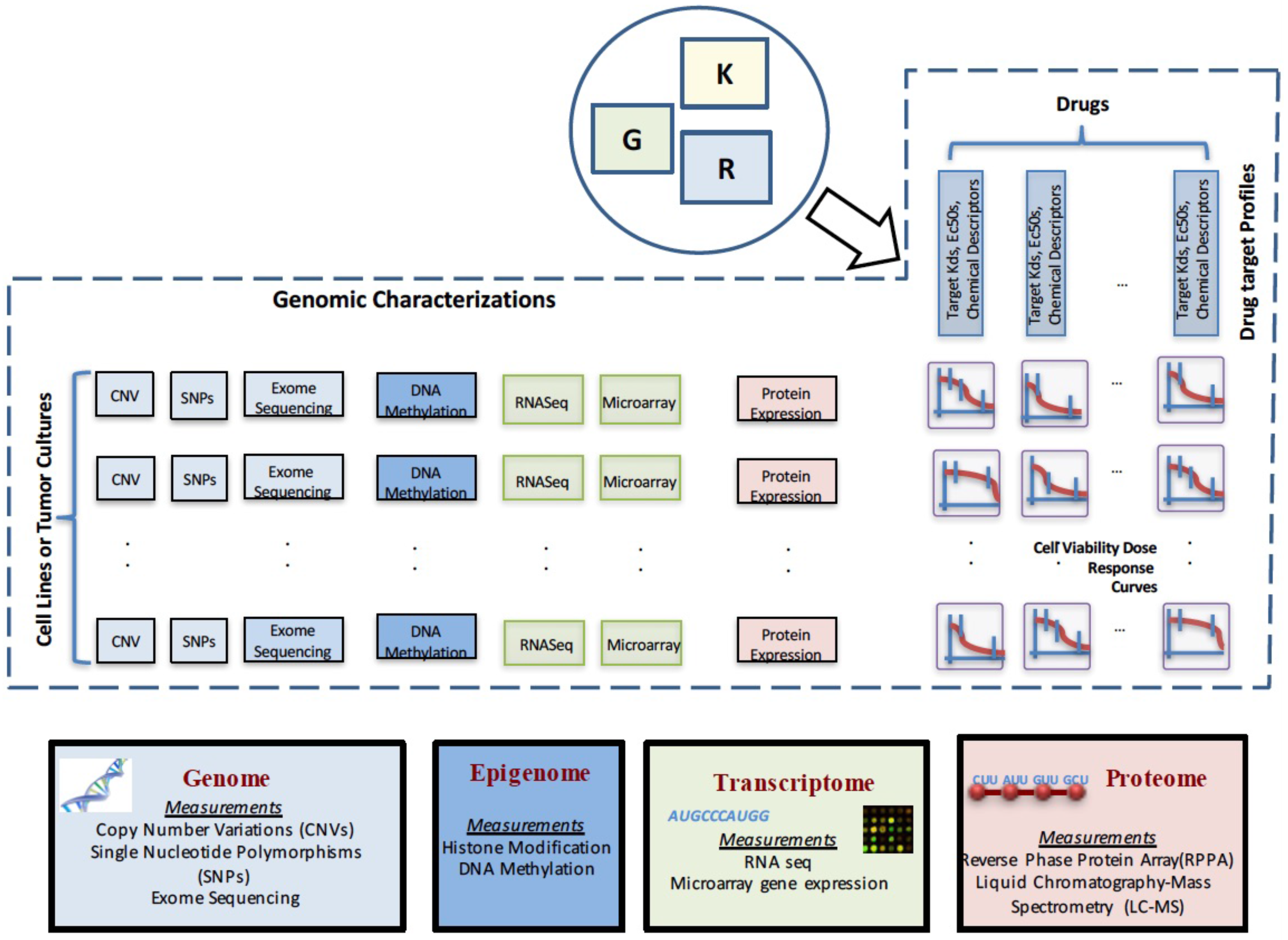
Figure 2.
Example dose response curve with commonly-used curve parameters.

Figure 3.
Average trajectory of generalization and training error with the increase in the number of features with a fixed number of training samples.
Figure 3.
Average trajectory of generalization and training error with the increase in the number of features with a fixed number of training samples.

Figure 4.
Structure of deep neural networks.

Figure 5.
Protein and drug interactions among top features selected in gene expression data. The top 50 genes selected from gene expression data are passed to the STRING database to find protein-protein interaction. Then, this new network is passed to Cytoscape using the CyTargetLinker App to extend the Protein-Protein (PP) interactions in a 7759 drug database (DrugBank); only the elements marked with an * are displayed in this network.
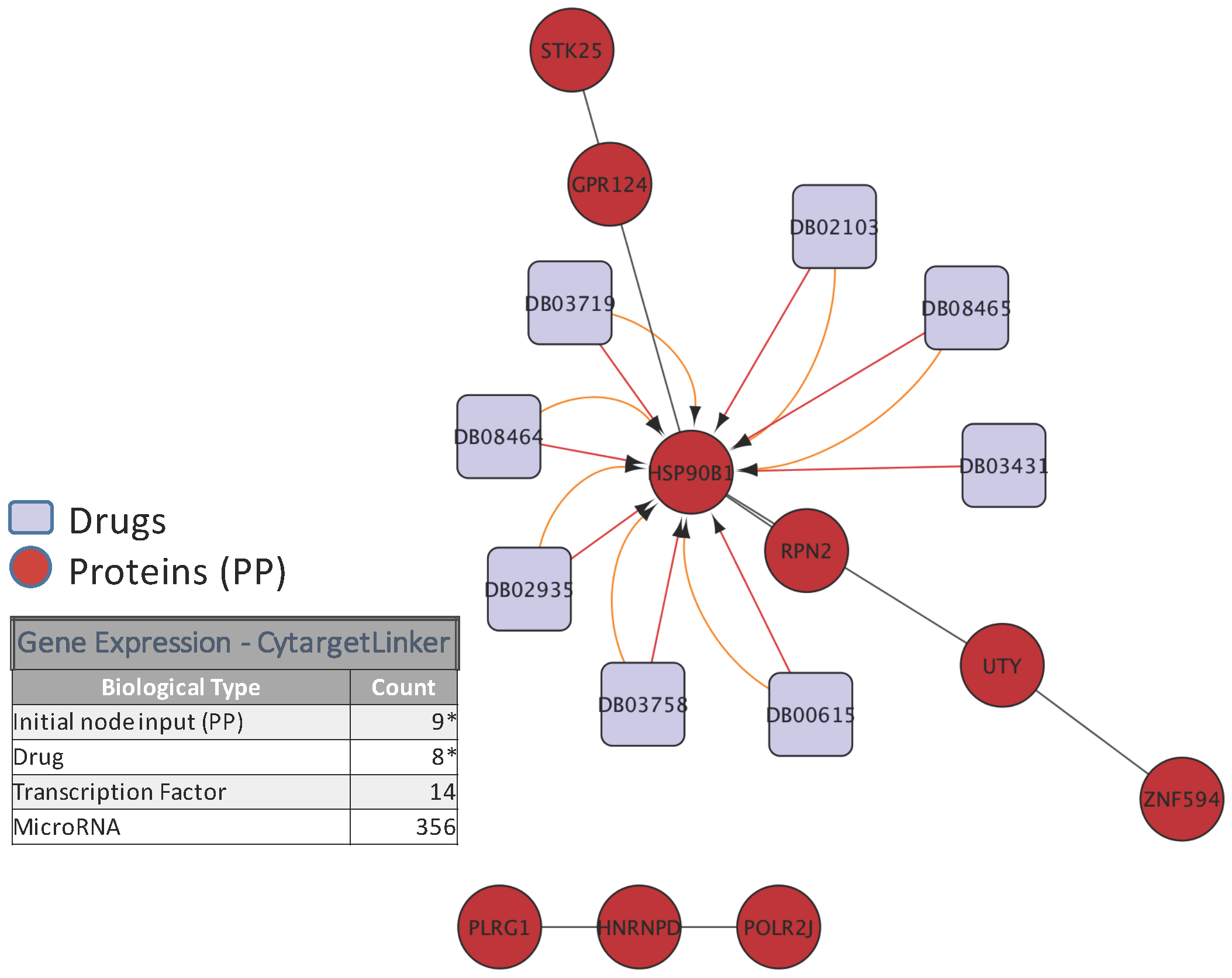
Figure 6.
(a) Protein and drug interactions among top features selected in the RPPAdata; (b) Outer ring showing details of the drug connection with CDK2; (c) Inner ring detail showing the CDK2 drug connectivity network from both the inner and outer rings. Images obtained from Cytoscape using the CyTargetLinker App (version 3.0.1). Only the elements marked with an * are displayed in this network.
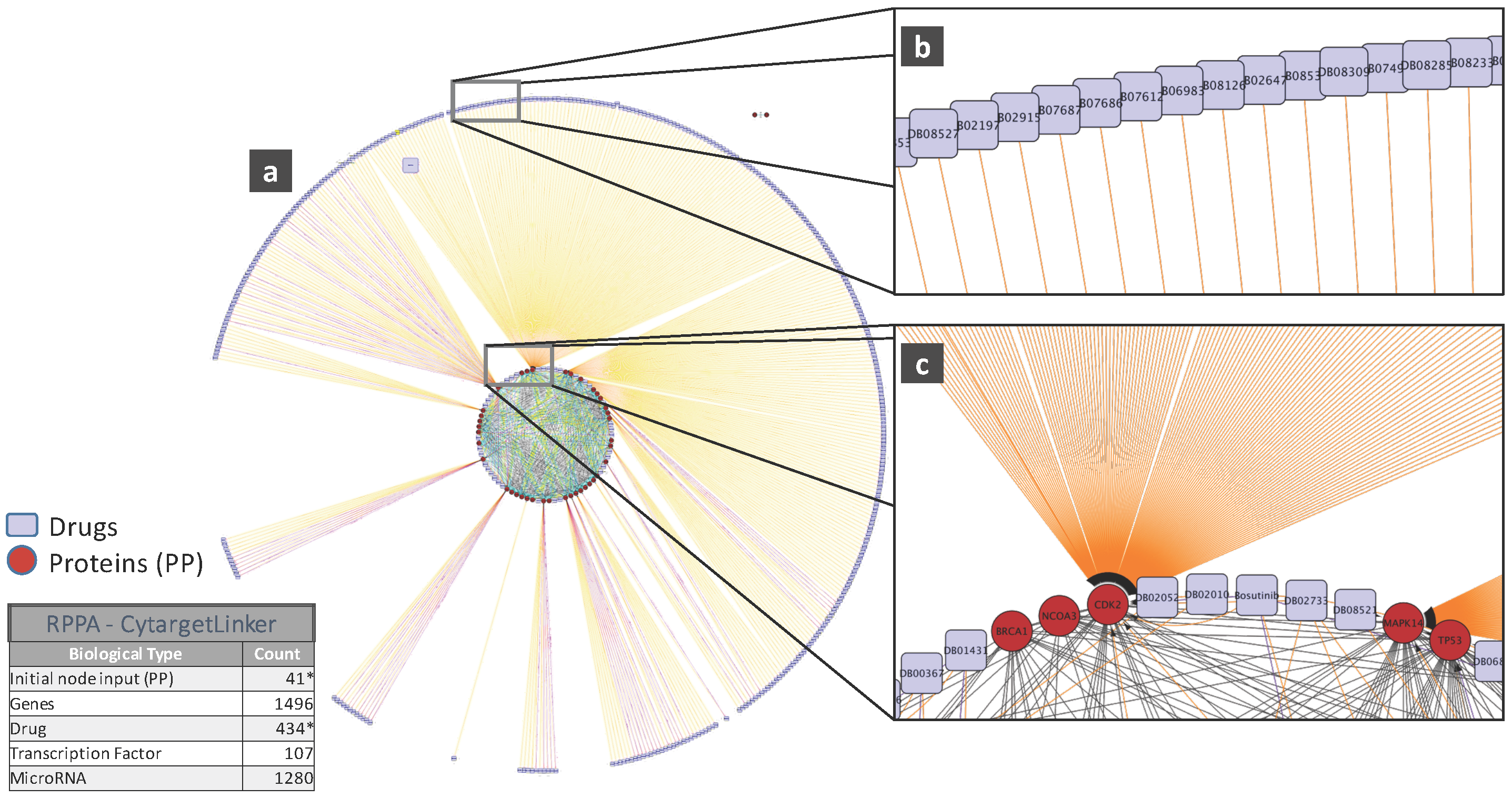

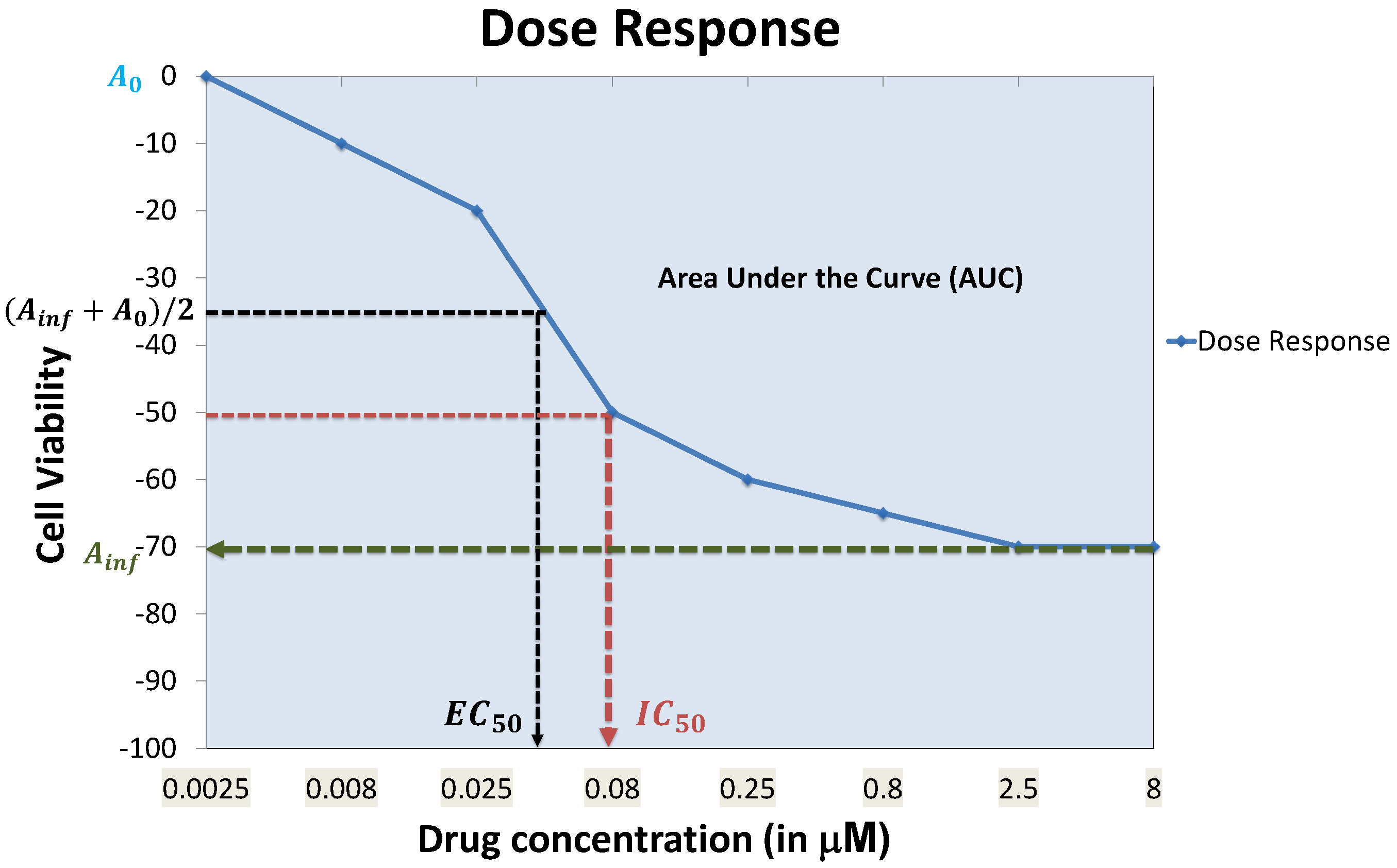
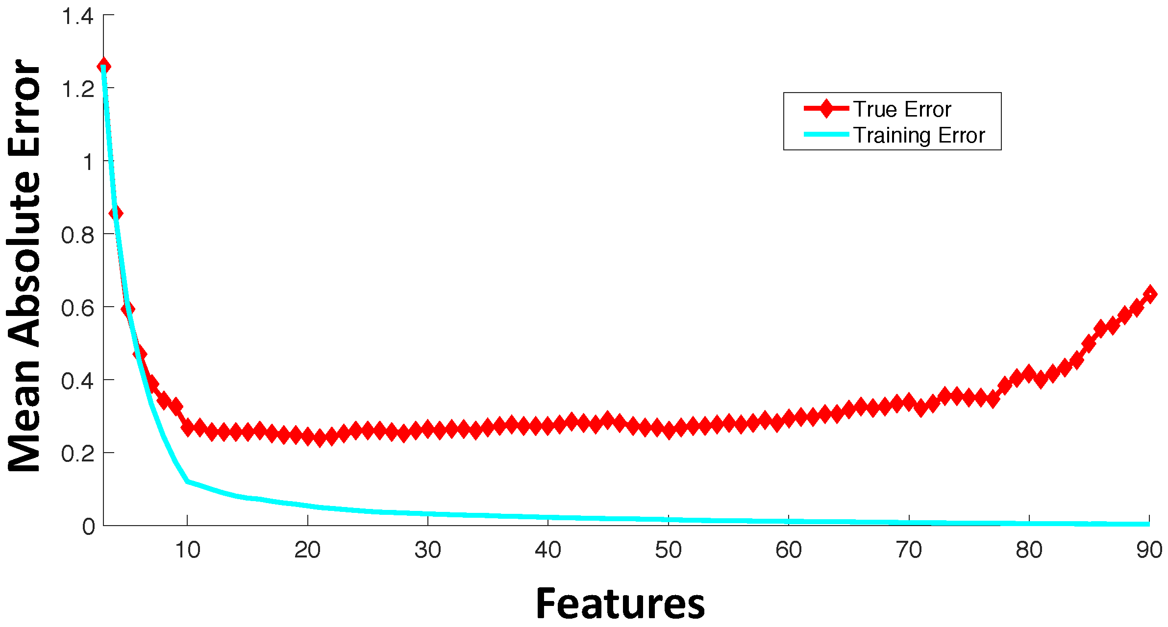
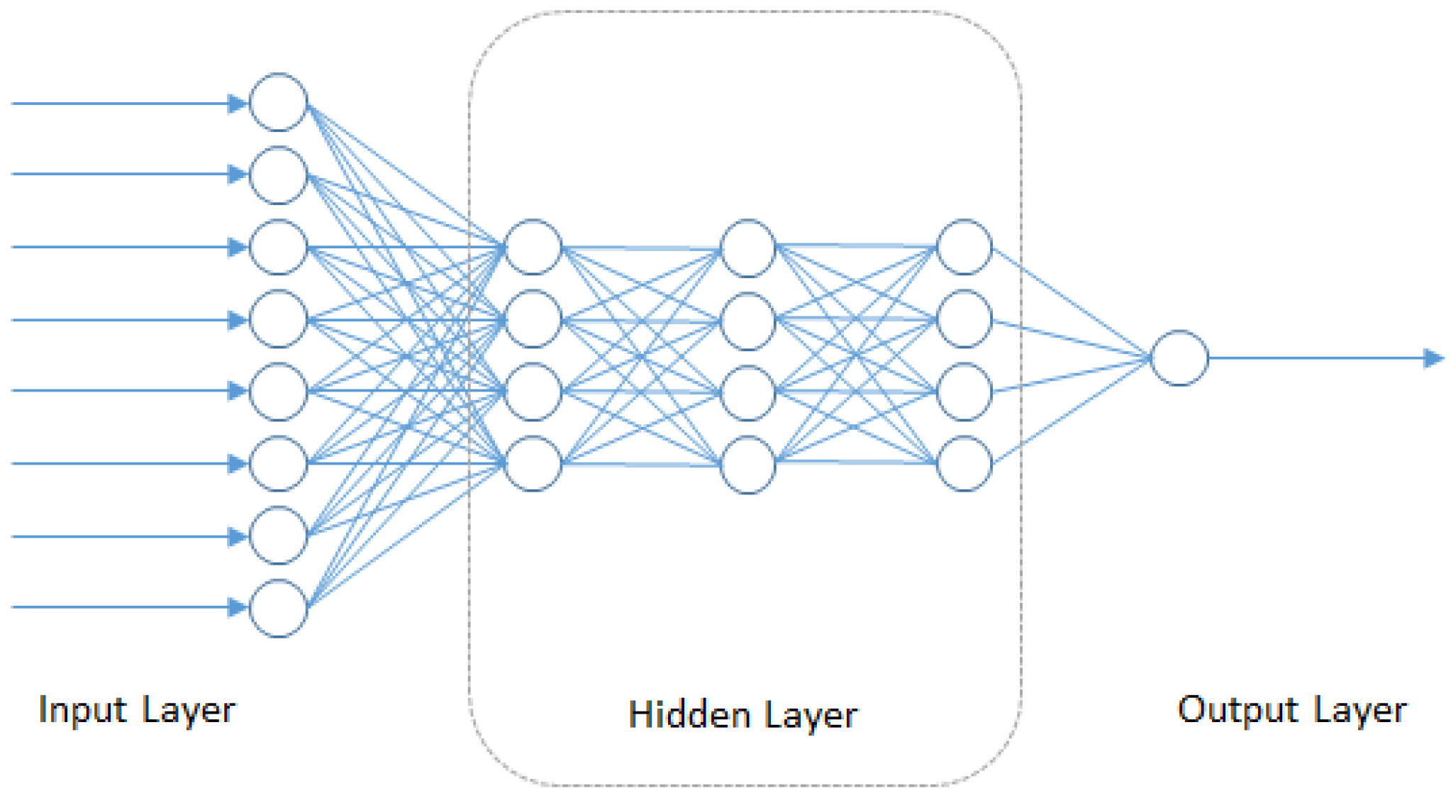
Table 1.
Prediction performance in the form of correlation coefficients between actual and predicted drug sensitivity for Elastic Net (EN), Kernelized Bayesian Multitask Learning (KBMTL), Random Forest (RF) and Deep Neural Network (DNN) for four drugs in the Cancer Cell Line Encyclopedia (CCLE) dataset.
| Drug Name | Correlation Coefficients | |||
|---|---|---|---|---|
| AZD0530 | 0.2149 | 0.2245 | 0.2577 | 0.1986 |
| Erlotinib | 0.3905 | 0.4100 | 0.4438 | 0.1341 |
| Lapatinib | 0.4758 | 0.4641 | 0.5127 | 0.3667 |
| Crizotinib | 0.3348 | 0.2647 | 0.3622 | 0.2609 |
© 2016 by the authors; licensee MDPI, Basel, Switzerland. This article is an open access article distributed under the terms and conditions of the Creative Commons Attribution (CC-BY) license (http://creativecommons.org/licenses/by/4.0/).
Share and Cite
MDPI and ACS Style
De Niz, C.; Rahman, R.; Zhao, X.; Pal, R. Algorithms for Drug Sensitivity Prediction. Algorithms 2016, 9, 77. https://doi.org/10.3390/a9040077
AMA Style
De Niz C, Rahman R, Zhao X, Pal R. Algorithms for Drug Sensitivity Prediction. Algorithms. 2016; 9(4):77. https://doi.org/10.3390/a9040077
Chicago/Turabian StyleDe Niz, Carlos, Raziur Rahman, Xiangyuan Zhao, and Ranadip Pal. 2016. "Algorithms for Drug Sensitivity Prediction" Algorithms 9, no. 4: 77. https://doi.org/10.3390/a9040077
Note that from the first issue of 2016, this journal uses article numbers instead of page numbers. See further details here.