Article

Linear Algorithms for Radioelectric Spectrum Forecast

1
Faculty of Technology, Universidad Distrital Francisco José de Caldas, Bogota 110231, Colombia
2
Industrial and Systems Engineering Department, Faculty of Engineering, Universidad Nacional de Colombia, Bogota 111321, Colombia
3
Electrical Engineering Department, Universidad Autónoma Metropolitana Iztapalapa, Mexico City 09340, Mexico
*
Author to whom correspondence should be addressed.
Algorithms 2016, 9(4), 82; https://doi.org/10.3390/a9040082
Submission received: 2 August 2016 / Revised: 25 October 2016 / Accepted: 28 November 2016 / Published: 2 December 2016

Abstract

:
This paper presents the development and evaluation of two linear algorithms for forecasting reception power for different channels at an assigned spectrum band of global systems for mobile communications (GSM), in order to analyze the spatial opportunity for reuse of frequencies by secondary users (SUs) in a cognitive radio (CR) network. The algorithms employed correspond to seasonal autoregressive integrated moving average (SARIMA) and generalized autoregressive conditional heteroskedasticity (GARCH), which allow for a forecast of channel occupancy status. Results are evaluated using the following criteria: availability and occupancy time for channels, different types of mean absolute error, and observation time. The contributions of this work include a more integral forecast as the algorithm not only forecasts reception power but also the occupancy and availability time of a channel to determine its precision percentage during the use by primary users (PUs) and SUs within a CR system. Algorithm analyses demonstrate a better performance for SARIMA over GARCH algorithm in most of the evaluated variables.

1. Introduction

Radioelectric spectrum occupancy is widely studied due to its importance for the construction of new spectrum assigning policies in emerging technologies, as well as in monitoring activities both in licensed and unlicensed bands. Real measurements for spectrum use within a determined band allow the corresponding authorities to guarantee that licenses meet local and regional spectrum regulations [1]. On the other hand, precise parameter estimates like time quantity and geographical region where the different spectrum band is actually used bring useful information to determine spectral opportunities for variant technologies within a domain. In this paper, such technologies correspond to a global systems for mobile communications (GSM) technology variant in the time domain [2].
The spectrum sensing in cognitive radio (CR) provides the necessary information about the status of the wireless channels, modeling and prediction of communications activity. This could contribute to spectral efficiency improvement efforts [3,4,5]. The prediction information of the channel status can be used by secondary users (SUs) to decide the sensing periods and channel occupancy duration for a single channel sensing scenario [6]. Besides, based on prediction information, SUs can select the channels with higher probability of vacancy in multi-channel wideband sensing scenarios [7], and also primary user (PU) occupancy models can be used as empty channel indicators replacing the spectrum sensing procedures [2,8]. A key issue for spectrum sensing operations is the evaluation of the so-called hidden node margin (HNM). The HNM has been evaluated in sharing scenarios between white space devices and digital terrestrial television systems [9].
Different initiatives for radioelectric spectrum channel modeling, mainly using deterministic and stochastic models, have been proposed [3,10,11,12,13,14,15,16]. Differences among those proposals and the present work lie in that in the first initiatives, the duty cycle (the average percentage of the channel utilization) time series is modeled for different types of channels, whereas the proposal presented here models the time series for received power in three GSM channels with different occupancy levels. For this purpose, firstly we used seasonal autoregressive integrated moving average (SARIMA) algorithm, which is adequate for analyzing time series with seasonality, in accordance with different studies [13,14,15]. Secondly, the generalized autoregressive conditional heteroskedasticity (GARCH) algorithm, which had been applied in traffic modeling and forecast for different communications networks, was also used [17,18,19].
The evaluation of the results obtained in algorithm forecasts is based on the following variables: channel availability time (the time interval where the channel is not used by the PUs), channel occupancy time (time interval where the channel is used by the PUs), observation time and error criteria analysis (symmetrical mean absolute percentage error, SMAPE, mean absolute percentage error, MAPE, and mean absolute error, MAE) [20,21,22].

2. Theory and Background

GARCH and SARIMA are deployed in a time series that is assumed as linear and with a known statistical distribution. As presented below, this is partially met in long-term analysis of time series measurements.

2.1. Seasonal Autoregressive Integrated Moving Average Algorithm

In general, if a time series exhibits potential seasonality indexed by s, then using a multiplied SARIMA(p,d,q)(P,D,Q)s algorithm is advantageous, where d is the level of non-seasonal differencing, p is the autoregressive (AR) non-seasonal order, q is the moving average (MA) non-seasonal order, P is the number of seasonal autoregressive terms, D is the number of seasonal differences, and Q is the number of seasonal moving average terms. The seasonal autoregressive integrated moving average algorithm of Box and Jenkins [23] is given in the Equation (1),
p ( B ) Φ p ( B s ) d s D x t = θ q ( B ) Θ Q ( B s ) e t
where B is the backward shift operator, xt is the observed time series of load at time t, et is the independent, identical, normally distributed error (random shock) at period t; s D x t = ( 1 B s ) D x t , ɸp(Bs) and ΘQ(Bs) are the seasonal AR(p) and MA(q) operators, respectively, which are defined in Equations (2) and (3),
Φ p ( B s ) = 1 Φ 1 B s Φ 2 B 2 s Φ p B P s
Θ Q ( B s ) = 1 Θ 1 B s Θ 2 B 2 s Θ Q B Q s
where ɸ1, ɸ2,…, ɸp are the parameters of the seasonal AR(p) model, Θ1, Θ2,…, ΘQ are the parameters of the seasonal MA(q) [24].
The Box-Jenkins methodology consists of four iterative steps [25]:
  • Step 1: Identification. This step focuses on the selection of d, D, p, P, q and Q. The number of the order can be identified by observing the sample autocorrelations (ACF) and sample partial autocorrelations (PACF).
  • Step 2: Estimation. The historical data is used to estimate the parameters of the tentative model in Step 1.
  • Step 3: Diagnostic checking. Diagnostic test is used to check the adequacy of the tentative model.
  • Step 4: Forecasting. The final model in Step 3 is used to forecast the values [26].

2.2. Generalized Autoregressive Conditional Heteroskedastic Algorithm

An important number of models, most of which have the property that conditional variance depends on past, have been proposed for capturing special data characteristics. Algorithms commonly used are those with autoregressive conditional heteroskedasticity (ARCH) introduced in [27] and generalized ARCH (GARCH) given by [28]. Modeling ARCH-GARCH considers conditional error variance as a compression function of the past of the series.
ARCH modeling usually requires a great number of lags (q), and therefore a great number of parameters. This might yield a model with a great number of parameters, which is in opposition to the parsimony principle. This fact drives many times to difficulties when using the model to describe data in an adequate way. On the contrary, a GARCH model uses an inferior quantity of parameters, which makes it preferable to an ARCH model [29,30,31]. In this paper, the GARCH algorithm with order p ≥ 0 and q ≥ 0 for the discrete-time stochastic process rt is expressed in Equations (4) and (5)
r t = μ + c ,   ε t ~ N ( 0 , 1 )
σ t 2 = α 0 + i = 1 q α i r t i 2 + j = 1 p β j σ t j 2
where εt is an independent and identically distributed process with a zero mean and one standard deviation, µ is the mean constant offset, σt2 is variance, and α0 is the constant in the conditional variance. Unknown parameters for model are α0, αi and βj for some positive integer p, q.
Just as in an ARIMA model, ACF and PACF are useful for p and q order identification in a GARCH(p,q) process [30].

3. Case Study and Experiment Procedure

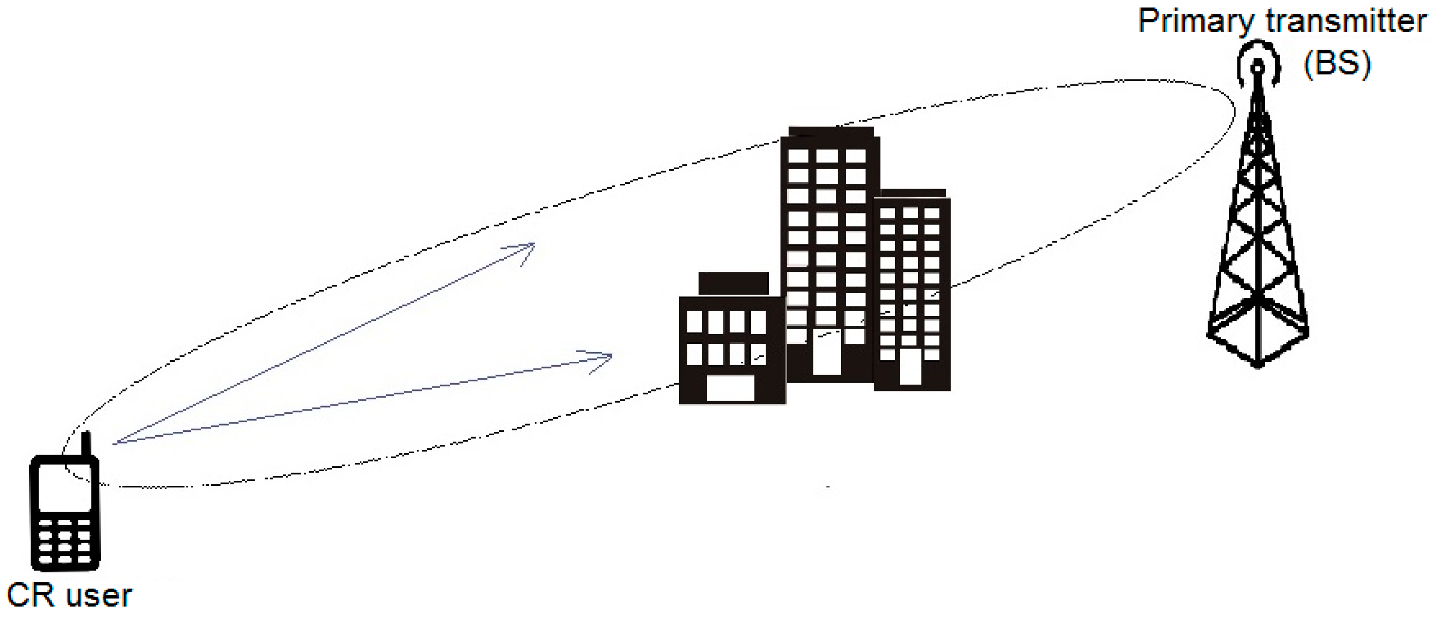
The decision to carry out this study was made during the spectrum measurements campaign held in Bogota-Colombia where we obtained the measurements employed here from spectrum occupancy study previously carried out [1,32]. The band analyzed was the GSM 850 MHz, as it is a band constantly used and viable for analysis in time function with conventional equipment, like a spectrum analyzer. The measurements used in this study correspond to a week, from 23 December to 29 December 2012. In some studies [33], it has been indicated that a reasonable option to obtain representative data without any a priori information about a band is to consider measurement periods of at least 24 h in order to avoid under or overestimating frequency bands occupancy with some temporary patterns. While a 24-h measurement period could be thought of as adequate in order to properly characterize the activity of determined spectrum bands [34], in this research 7 days were analyzed, including patterns for workdays and weekends. Additionally, this time period is sufficient to measure occupancy in mobile networks with low use, as indicated in [2,34].
The channels to be modeled were selected after measuring the duty cycles of 60 channels at GSM band. From these, three channels with different occupancy levels (high, medium and low), were chosen. 
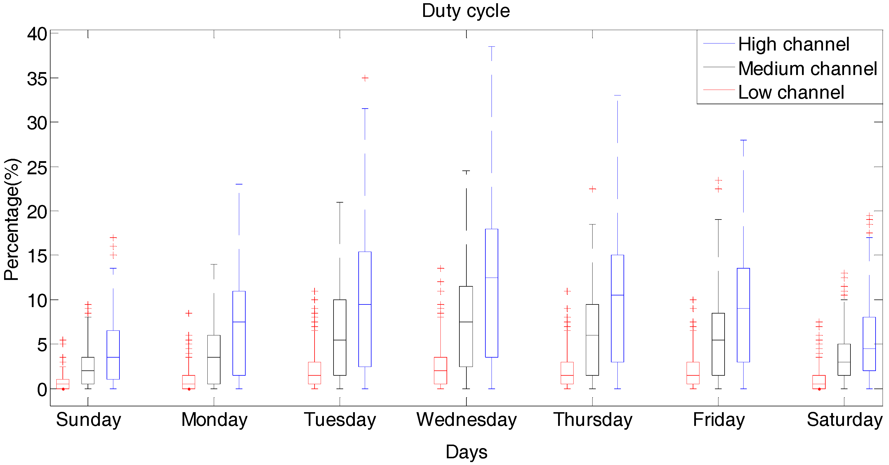
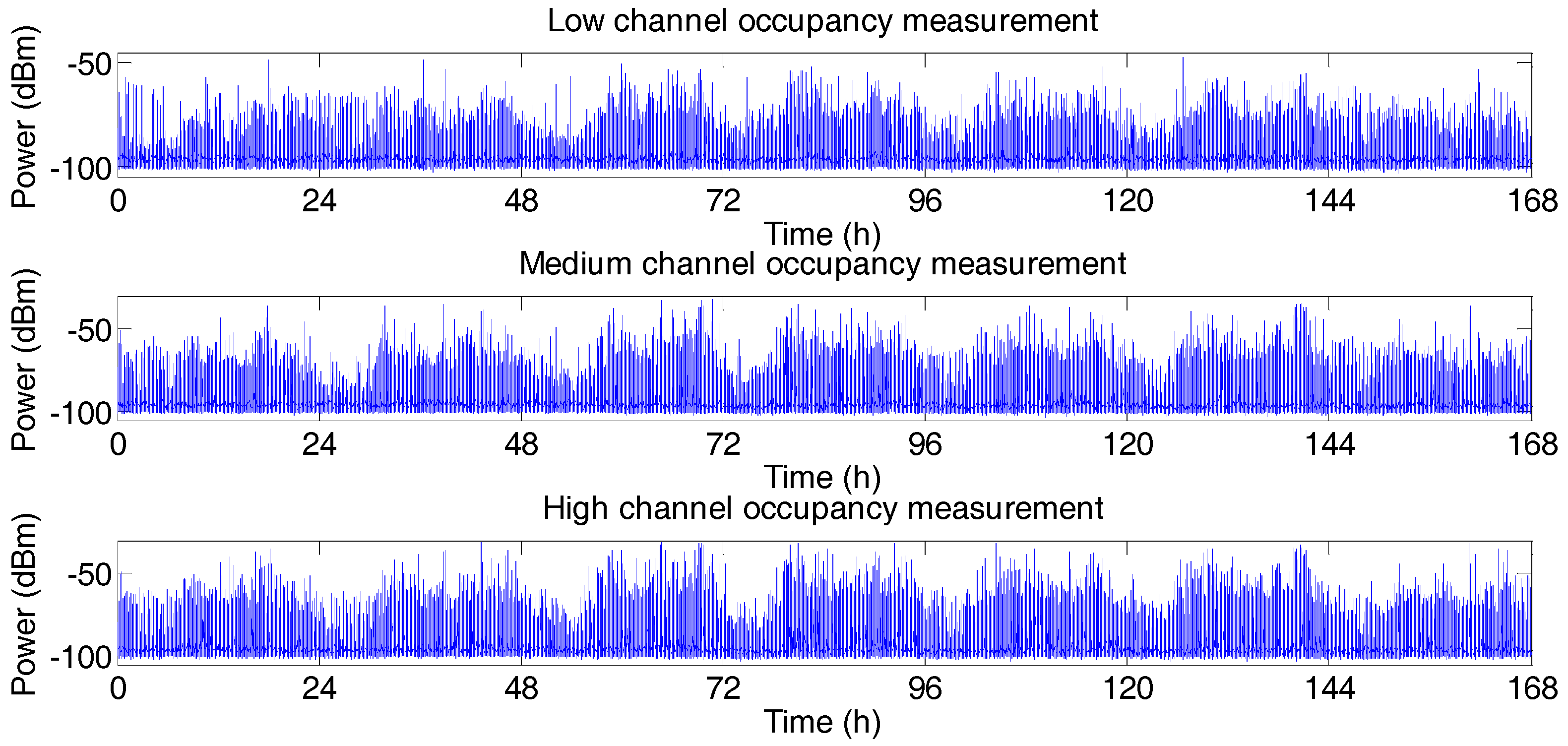
Figure 1 presents results of power measure for three downlink channels during a week, with different power level. Spectrum analyzer configuration for this band was the following: a resolution bandwidth of 100 kHz with a sweep time of 290 ms, which guarantees GSM signal detection with a bandwidth of 200 kHz. Daily duty cycles from PUs at selected channels are shown in Figure 2. Threshold (λ) used, which for this event is of −89 dBm, was obtained from Equation (6) with a probability of false alarm (Pfa) of 1% [35]. λ which is above of the detected noise floor of −102 dBm [1],
P f a = Γ ( m , λ 2 ) Γ ( m )
where Г(.) y Γ(. , .) are complete and incomplete gamma functions, respectively, and m is the product of time times bandwidth.
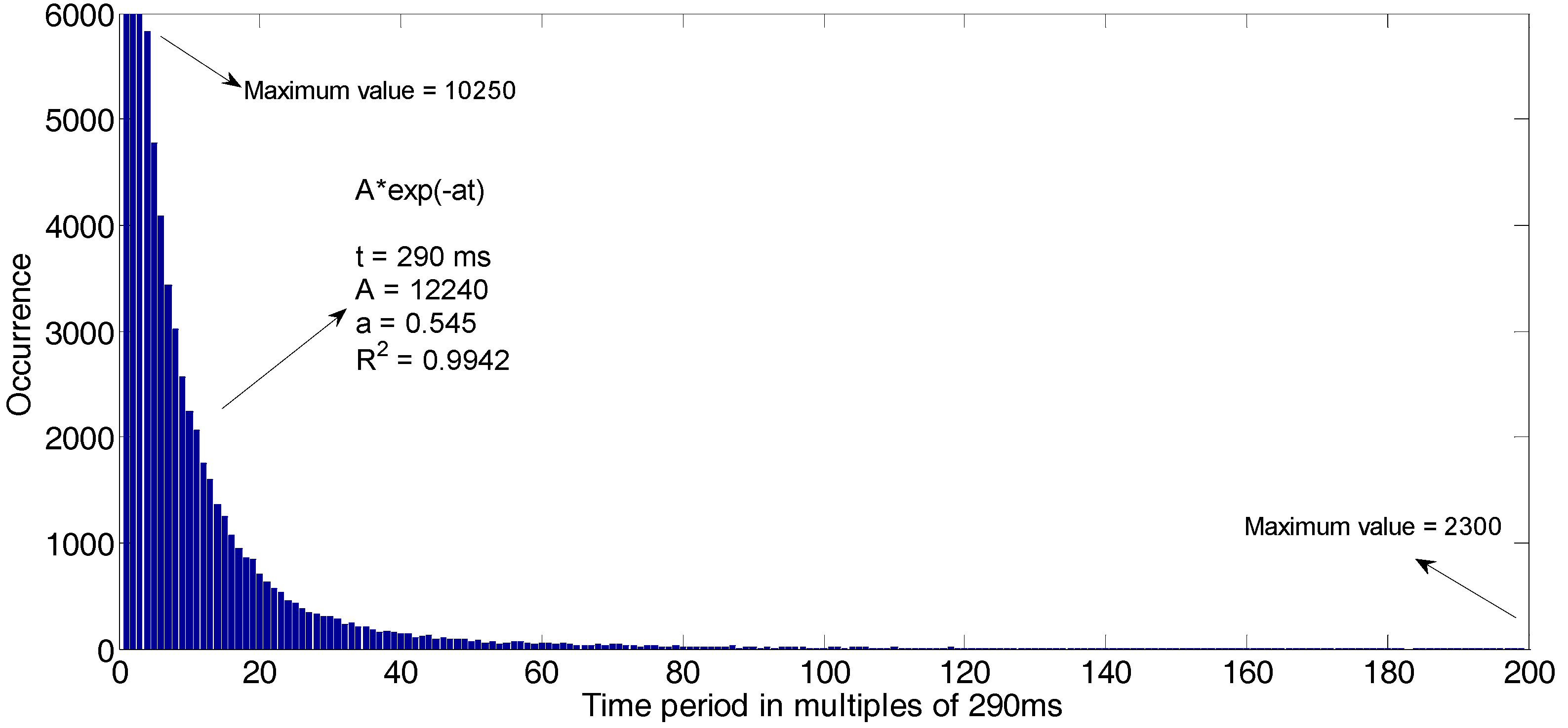
In this work the HNM is calculated from the differences between measurements of received power performed outside at street level and indoors, in a building. These measurements were performed with a discone-type antenna and spectrum analyzer. The calculation allows analysis of the margin between a non-licensed device indoors, and a PU outdoors without interference due to shadowing. Table 1 shows the HNM found for each channel.
Figure 3, Figure 4 and 
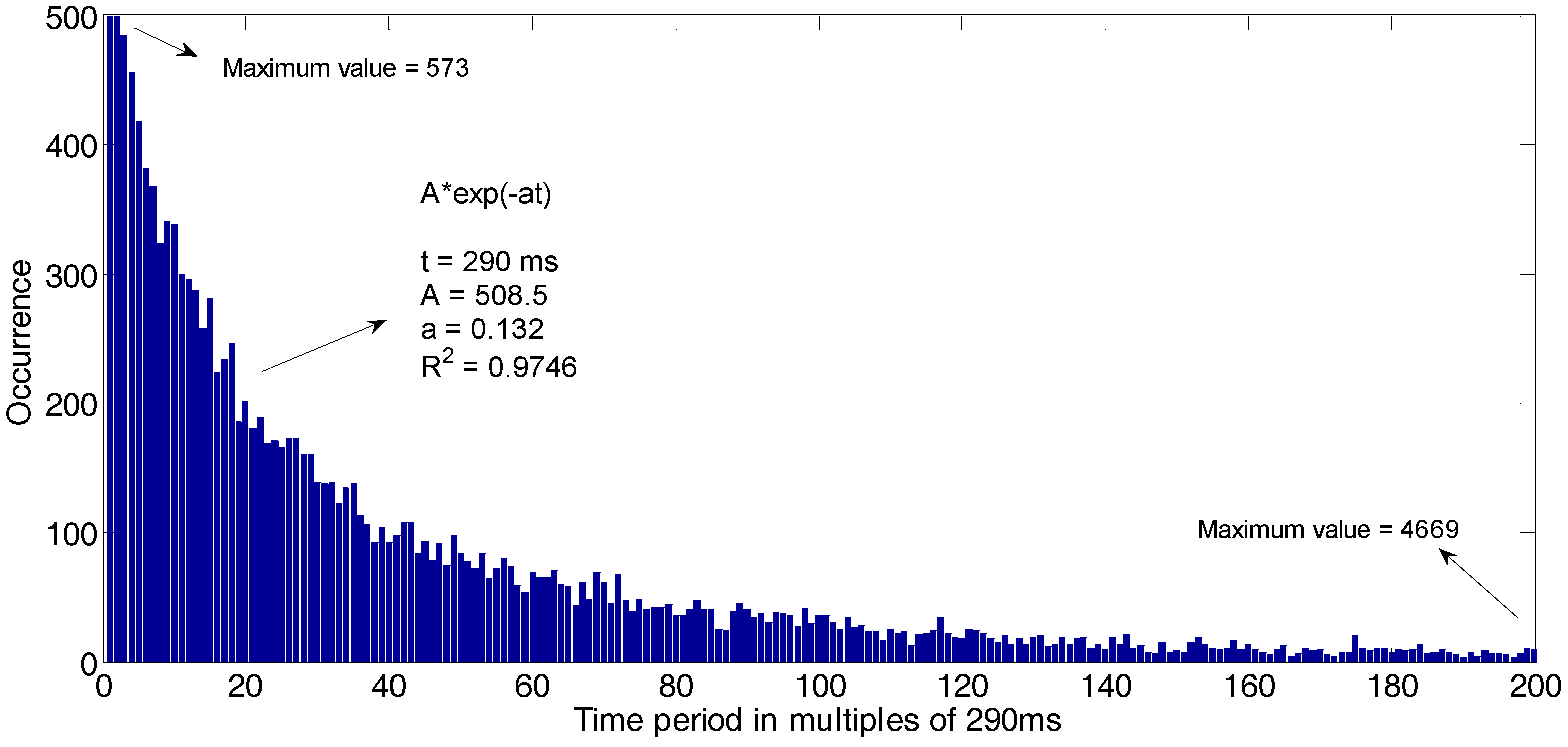
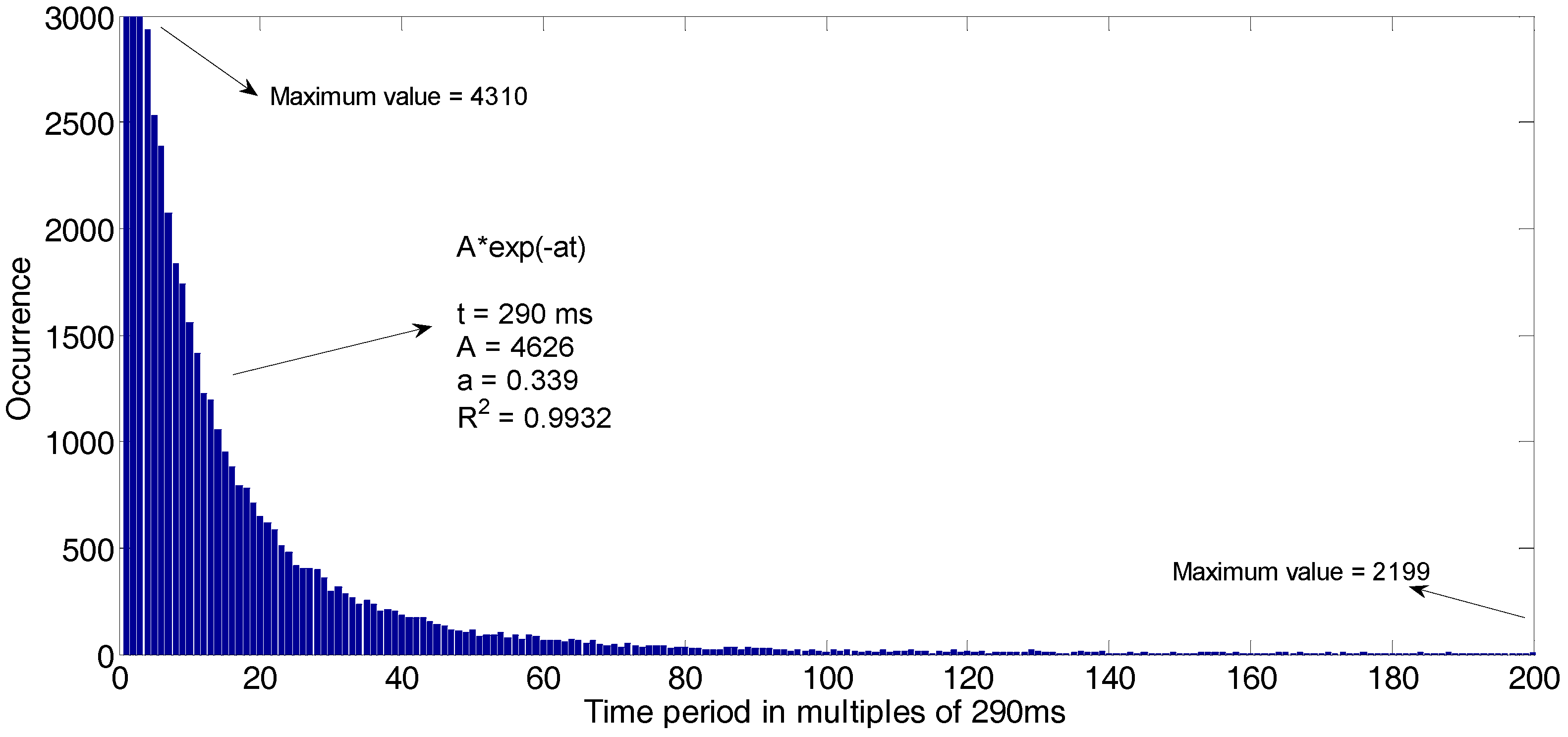
Figure 5 present histograms corresponding to opportunities distribution during time periods of GSM band channels; it is observed that such opportunities have an exponential behavior, whose approximate equations and the coefficient of determination (R2) are exhibited in each figure. Thus, the occurrence increases for the channel occupancy, especially for shorter time periods of use. For low, medium and high occupancy channels, total times of opportunities were approximately 84 h, 81 h and 78 h, respectively, which indicates relatively low occupancy [2].
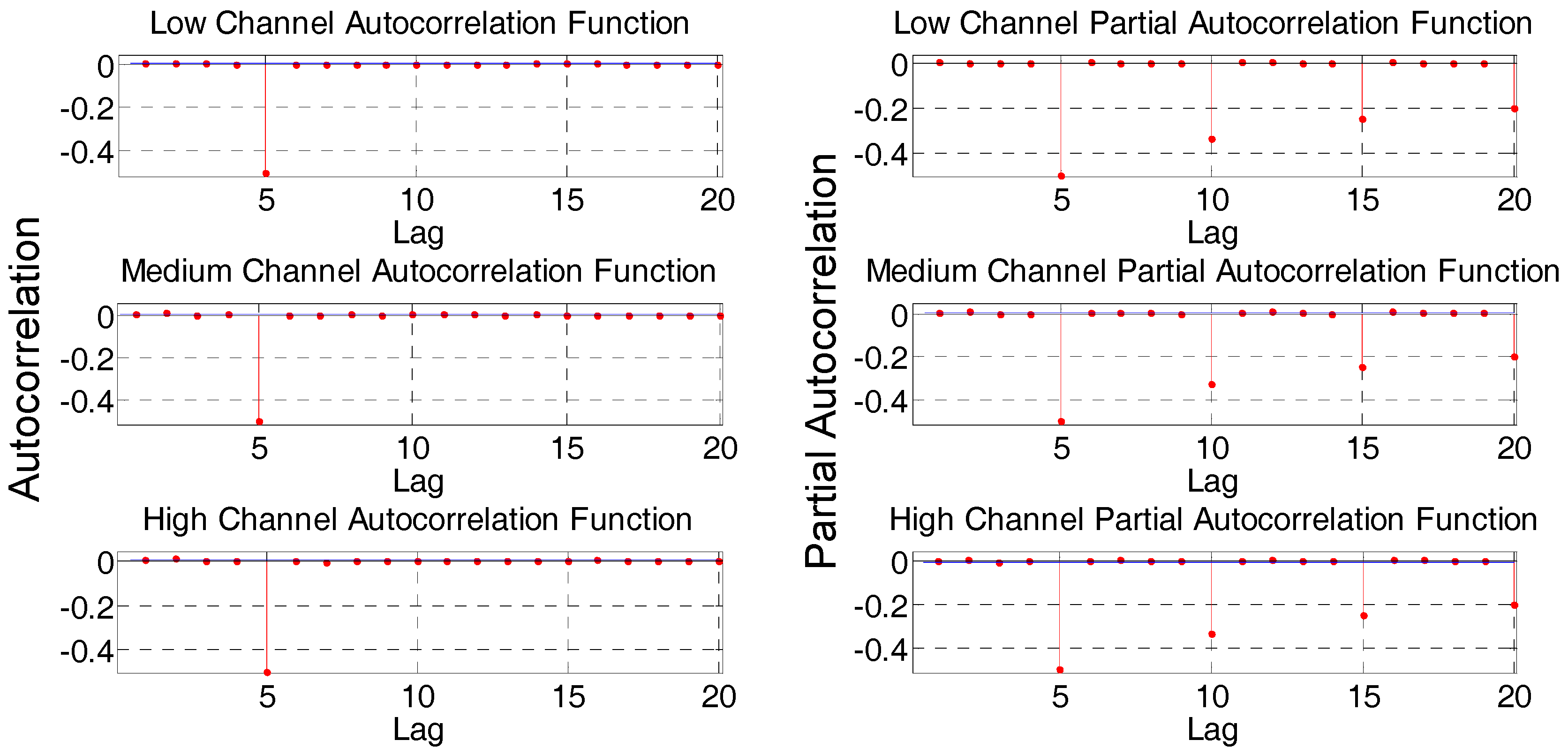
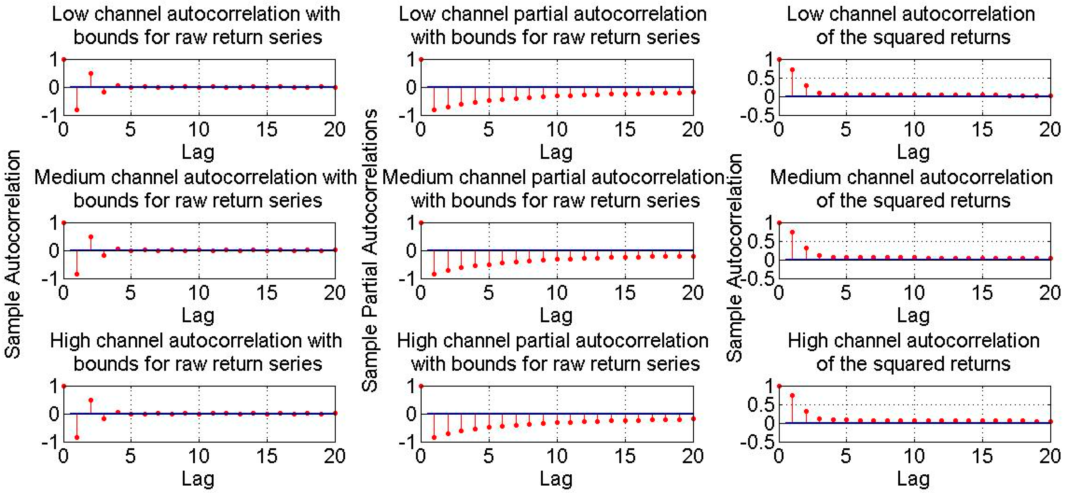
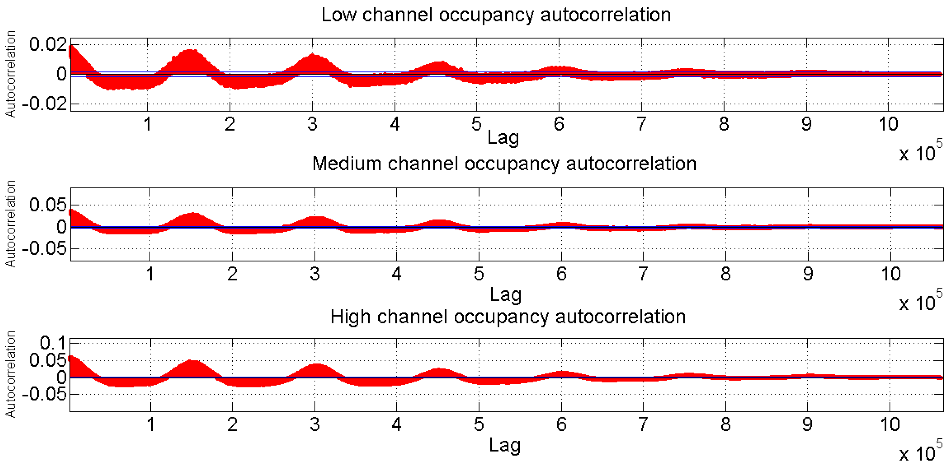
Following this, we proceeded to analyze the time series of measured channels over a week, which was equivalent to 1,062,514 samples. To do this, ACF is initially presented, as observed in Figure 6. ACF diagrams for the three channels presents forms which are alternately positive and negative, decaying to zero, the values are in 95%-confidence intervals, shown with the blue lines. Therefore, this indicates that there is correlation [2,26].
When analyzing channels stationarity of Figure 6, it is observed that the mean and variance are constant and similar to each other, on each one of the days from Monday to Friday. Therefore, measurements at the weekend are not taken into consideration when training the analyzed models, because the mean and variance are not similar and change in a significant way with regard to the measurements from Monday to Friday.

3.1. Design of SARIMA Algorithm
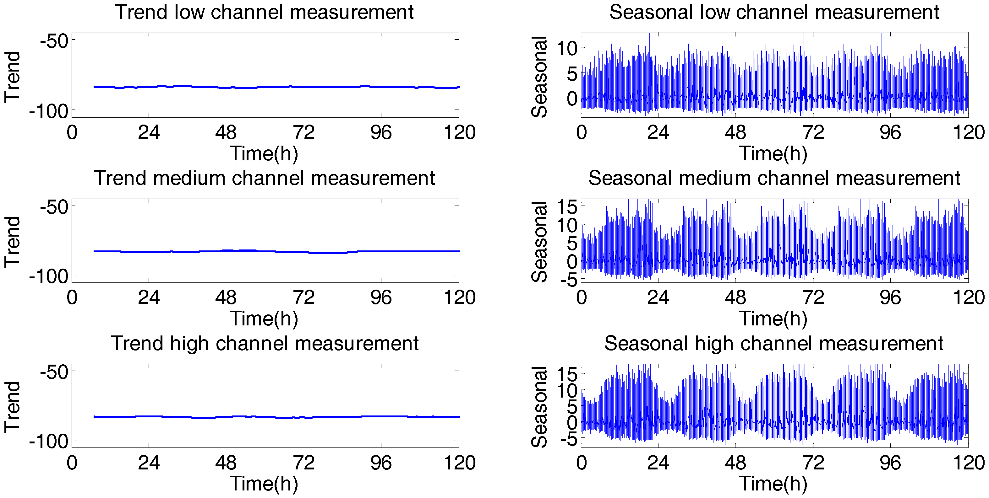
In Figure 7 the trend and seasonality are presented in occupancy level for the three channels. Seasonality had a period of 24 h, practically without trend and with stationary components, which makes possible the use of a SARIMA model to forecast behavior of the GSM channels [26].
Delay difference s, which for this event is selected as five (∆5), was equivalent to the number of days of the week in which the signal was stationary [15]. Applying the augmented Dickey–Fuller test [36], in the series of three channels from Monday to Friday, the null hypothesis of unit root is rejected, which indicates stationarity. In order to find the parameters of SARIMA(p,d,q)(P,D,Q)s model, ACF and PACF were calculated for ∆5 of respective channels, as shown in Figure 8.
Using Box-Jenkins methodology [23], Figure 8 shows that PACF of ∆5 decays to zero with a seasonal pattern, and crosses confidence level initially in lag 5 for negative side. This suggests that a term non-seasonal AR(1) could be used, and a seasonal MA(5) could be added.
In order to avoid forecast overestimation (small variance and big errors), the Akaike information criterion (AIC) [37] was selected to evaluate different reasonable combinations, as is observed in Table 2. Thus, selected models were: SARIMA(1,0,5)(1,0,1)5, SARIMA(1,0,5)(0,0,1)5 and SARIMA(1,0,5)(0,0,1)5, for occupancy levels of low, medium and high channels, respectively, and the characteristic equations, in the same order are:
( 1 0.0135 B ) ( 1 0.55 B 5 ) ( 1 B ) ( 1 B 5 ) x t = ( 1 0.997 B 5 ) ( 1 0.546 B 5 ) e t
( 1 0.0192 B ) ( 1 + 0.996 B 5 ) ( 1 B ) ( 1 B 5 ) x t = ( 1 + 0.0085 B 5 ) e t
( 1 0.0199 B ) ( 1 0.016 B 5 ) ( 1 B ) ( 1 B 5 ) x t = ( 1 0.994 B 5 ) e t

3.2. Design of GARCH Algorithm

When analyzing in detail the large amount of acquired information, the existence of standard deviation was observed; therefore the GARCH algorithm was used to forecast the behavior of measured series. Stochastic models ARIMA and SARIMA are methods for univariate modeling. The main difference among former models and GARCH model lies in the constant variance assumption.
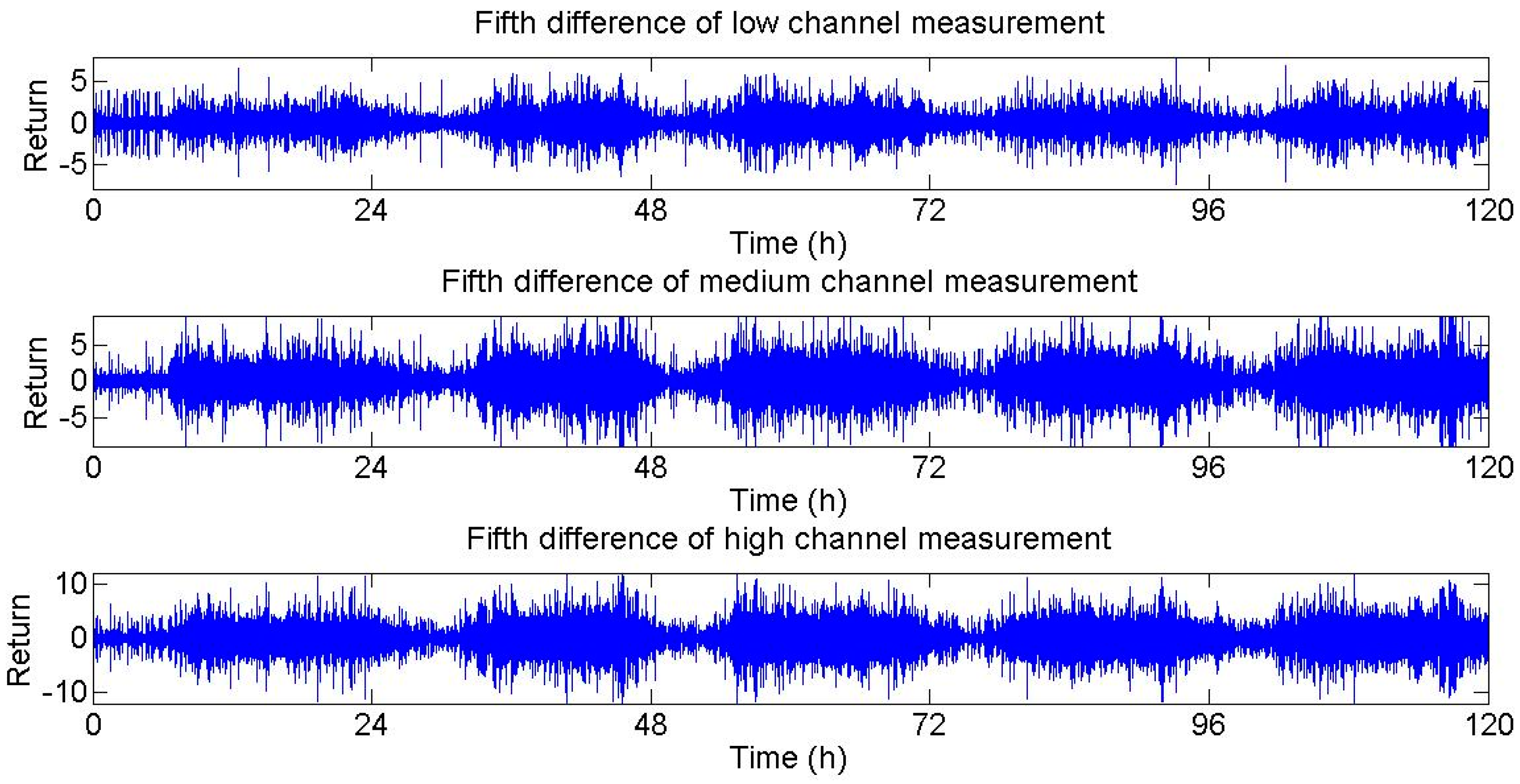
Even though for the developed algorithm there is stationarity in original signal from Monday to Friday, for this case the fifth difference is developed because there is a greater degree of stationarity. In Figure 9 the difference for each channel is presented. Channel measurements are converted into returns by logarithmic transformation. The logarithmic returns are defined in Equation (10),
r t = l n P t P t 1
where Pt is power value in time t and Pt−1 is power value in time t−1.
Now we present a formal statistical test in order to establish the presence of ARCH effects in the data and correlation. H = 0 implies that there exist no significant correlation as well as H = 1 indicates that there exists a significant correlation. In Table 3 and Table 4, all the p values show that Ljung-Box-Pierce Q-Test and Engle ARCH Test in lag 10, 15 and 20 are significant, revealing the presence of ARCH effects (heteroskedasticity), indicating that GARCH modeling is appropriate.
Dependence in data x1,…, xn was determined by computing correlations. This was done by representing the ACF.
If the time series is the result of a completely random phenomenon, the autocorrelation should be close to zero for all time-lag separations. Otherwise, one or more of the autocorrelations will be significantly different from zero. Another useful way to examine dependencies of the series is to revise the PACF, where the dependence of intermediate elements (those within the lag) is eliminated. In Figure 10, graphs of ACF, PACF and ACF of square returns present the existence of correlation in data of channel occupancy.
Below, in Table 5, Table 6 and Table 7, the evaluation and selection of the GARCH model for each channel was performed.
The GARCH model selection for each channel was done by fulfilling α i + β i < 1 criterion, so the model is stationary, and then taking into account the more proximate values to zero of MAE, MAPE and SMAPE from Table 5, Table 6 and Table 7. Therefore, the selected models for low, medium and high channel are GARCH(2,2), GARCH(0,2) and GARCH(0,1), respectively.
Parameters for low channel model were estimated and are presented in Table 8. GARCH(2,2), where α 1 + α 2 + β 1 + β 2 < 1 is fulfilled.
Thus, the model according to Table 8 is presented in Equations (11) and (12),
r t = 96.112 + ϵ t
σ t 2 = 0.003516 + 0.098255 σ t 1 2 + 0.90062 σ t 2 2 + 0.00029573 ϵ t 1 2
For medium channel, GARCH(0,2), model values presented in Table 9 are estimated.
Therefore, Equations (13) and (14) are obtained,
r t = 95.061 + ϵ t
σ t 2 = 5 + 0.085692 ϵ t 1 2 + 0.088298 ϵ t 2 2
For high channel, GARCH(0,1), the following parameters were obtained, as shown in Table 10.
Then the model is described in Equations (15) and (16),
r t = 94.585 + ϵ t
σ t 2 = 5 + 0.86058 ϵ t 1 2
ARCH-GARCH model analysis is based on evaluation of standardized residuals [31]. One assumption with GARCH model is that for a good model, residuals should follow a white noise process. This is to say that it is expected that residuals be at random, independent and identically distributed, following a normal distribution. 
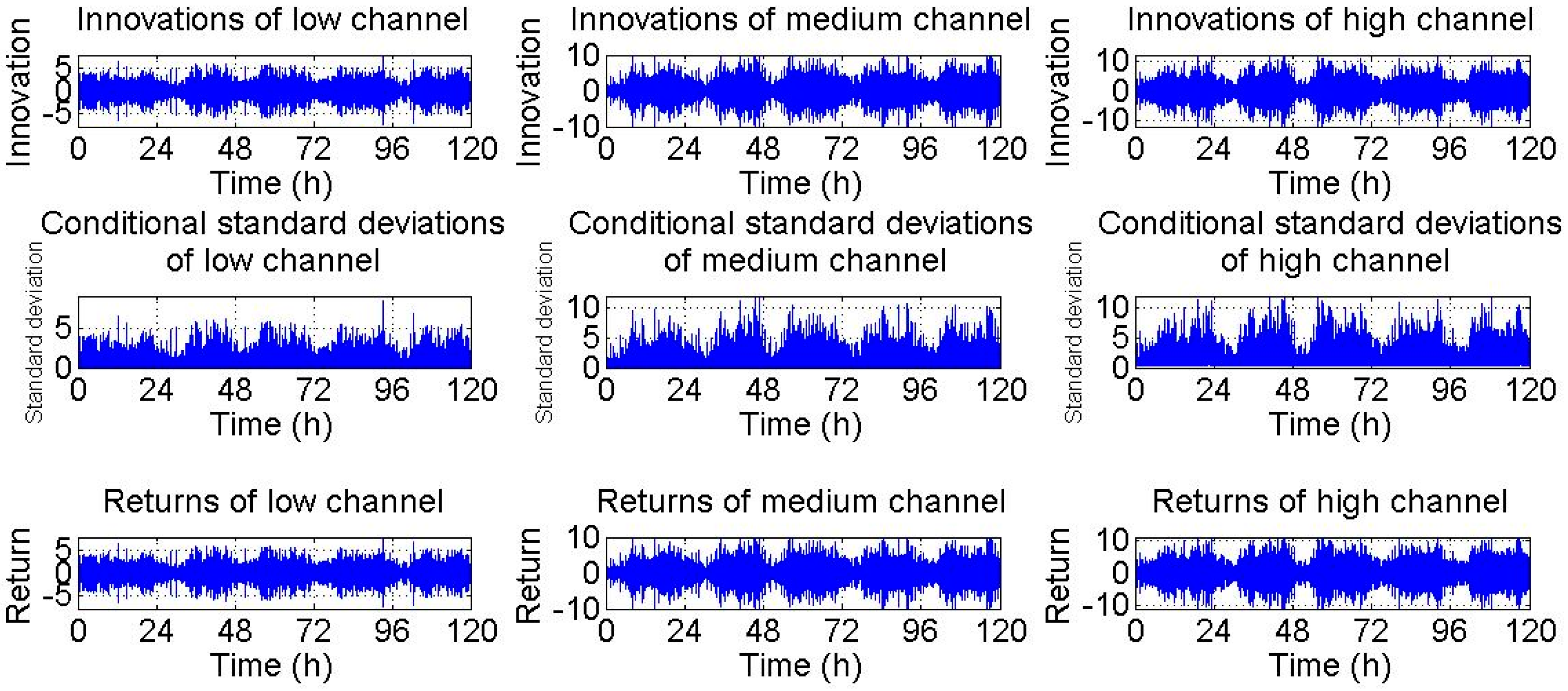
Figure 11 presents the relationship between innovations (residuals) derivate from adjusted model, the corresponding conditional standard deviations and returns. 
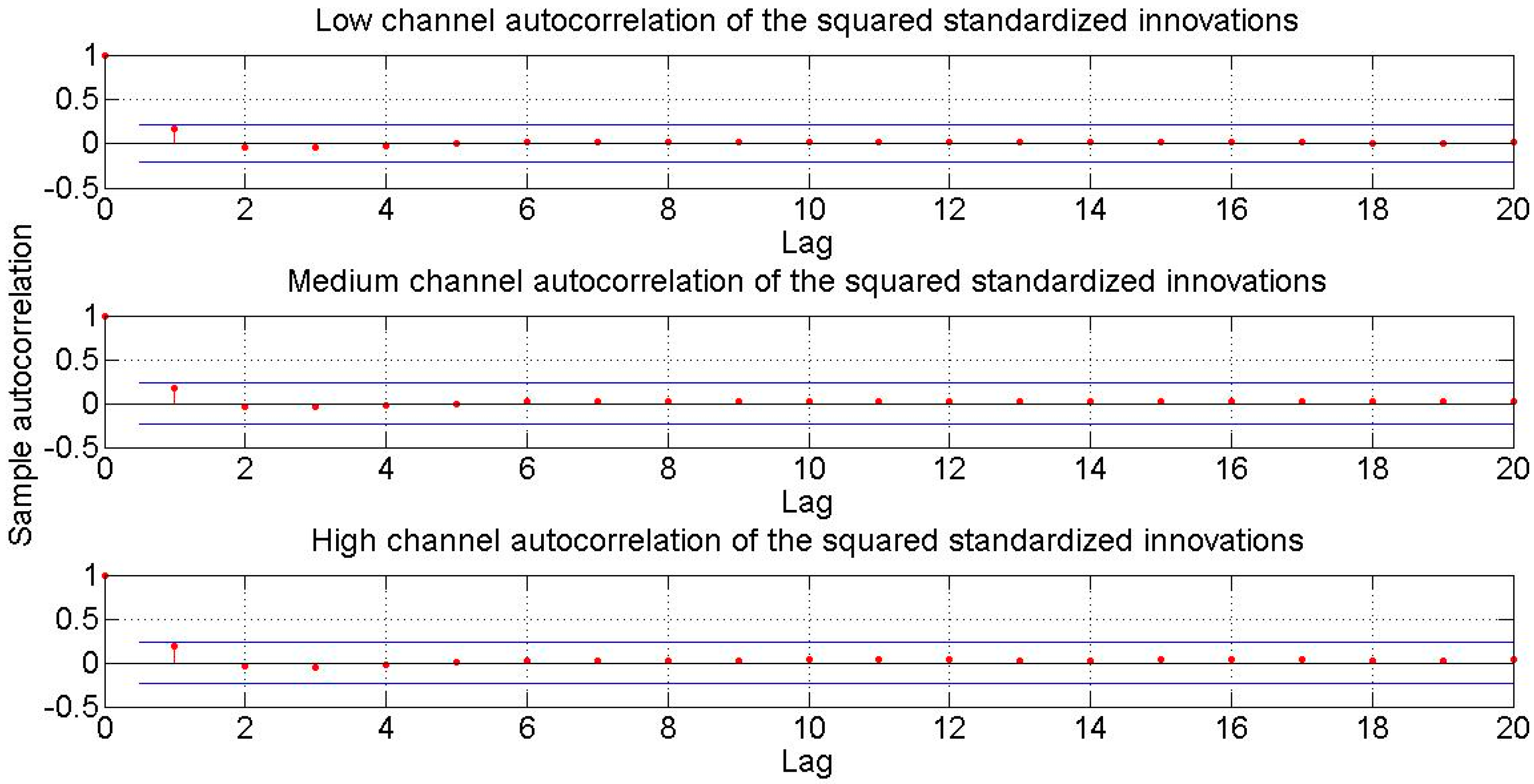
Figure 11 shows that both innovations and returns exhibit variations. In the following we intend to find out if by performing GARCH the autocorrelation of the standardized innovations disappears, which would indicate the effectiveness of GARCH model.
Figure 12 corresponds to the autocorrelation of the squared standardized innovations, in which correlation was not observed.
In Table 11 and Table 12, results of Ljung-Box-Pierce Q-Test and Engle ARCH test for later analysis are presented using standardized innovations. These tests indicate no presence of correlation or ARCH effects. We have GARCH effects and also correlation between innovations that disappear after treating the data. Therefore, the GARCH model is a proper model for explaining the variances of the three channels.
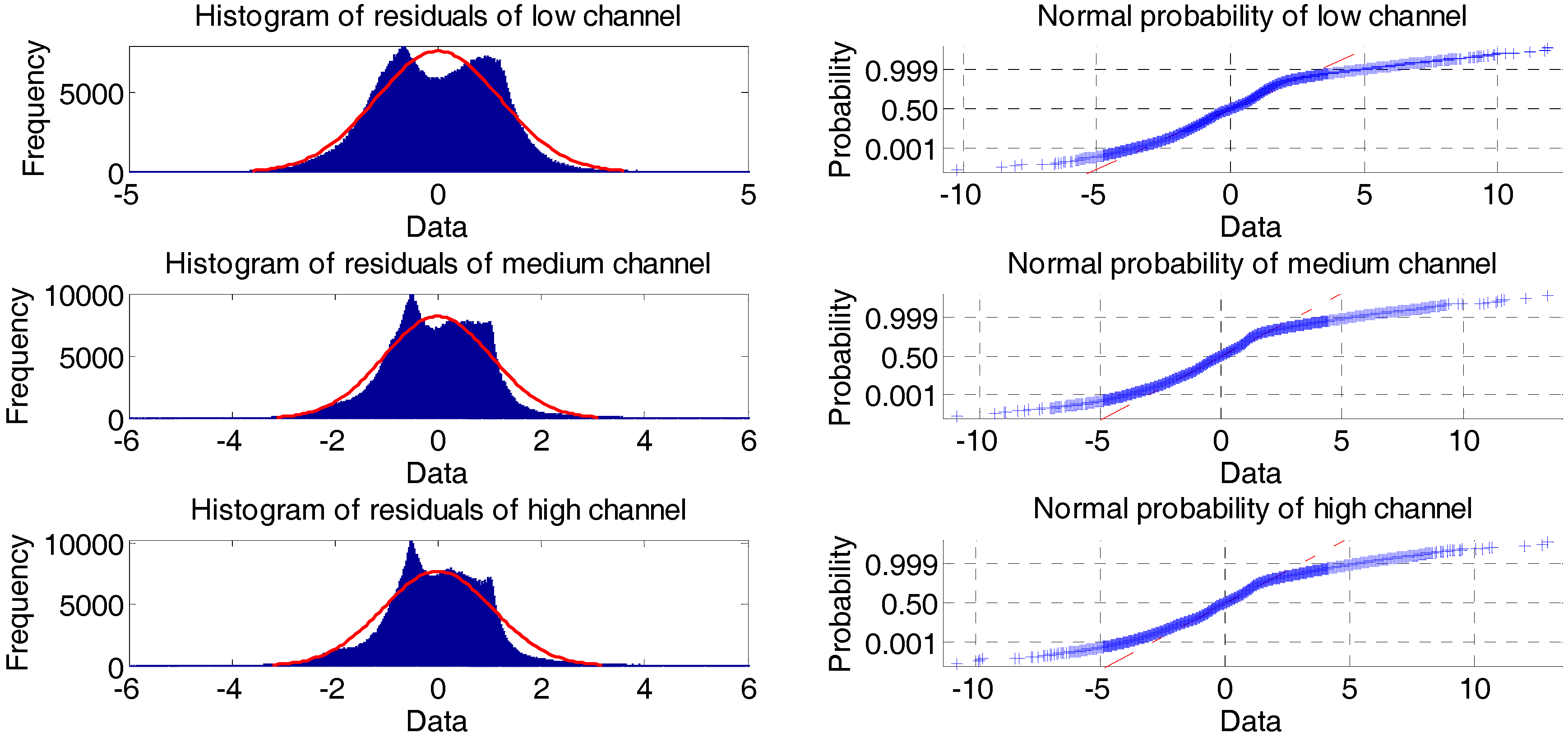
Normality verification was performed by analyzing histograms of residuals and normal probability graph, as shown in Figure 13. The histograms of the three channels shows that the residuals are normally distributed. In turn, the probability graph confirms that residuals respond to a normal distribution, since most of data are spread along the straight line.

4. Results and Discussion

In Figure 14 an example is displayed where there is application of the designed time series algorithms. Here, the interaction between the CR user and the primary base station (BS) is shown by received power from the primary transmitter. This is represented by the oval and the direction of the arrows. The CR user can forecast the power level it will receive from the primary BS.
In the example of Figure 14, in order to analyze the SARIMA and GARCH algorithms, the forecast of the power is performed by the CR user, making a comparison with the spectrum analyzer in which the measurements were made. However, this depends on the architecture of CR deployed in the environment. Due to the processor and power consumption being more limited in the CR user’s computer, use of infrastructure architecture is recommended, where the forecast is carried out by the CR BS. This provides a better processor than that of the CR user, and has no limitations on power consumption. However, there is a time period between data capture in the environment and the processing, which adds a delay to the response. This must not be ignored, but the forecast helps to reduce the negative impact of the delayed response.
The analysis of the precision of the forecast made with the SARIMA and GARCH algorithms is presented, as follows. Figure 15 shows the SARIMA algorithm forecasts obtained from Equations (7)–(9), and from GARCH algorithm based on Equations (11)–(16). This was contrasted with the power measured data of Friday from 5:00 p.m. to 6:00 p.m. This period was chosen since during this time an increased use of the channels by PUs was perceived.
In Figure 16 and Figure 17, availability and occupancy times of the measured and forecast channels are presented. Availability time allows us to analyze the precision with which SUs could use availability time in GSM channels for a CR system. In the same way, occupancy time examines the precision during time in which PUs use GSM channels. Average precisions obtained between actual and forecast data for availability times were: 82%, 54% and 60%, for the SARIMA algorithm; and 31%, 30% and 43%, for the GARCH algorithm, corresponding to channels with low, medium and high occupation, respectively. Average precisions for occupation times between real data and forecast data are equivalent to 58%, 77% and 78% for the SARIMA algorithm; and 44%, 46.6% and 44.2%, for the GARCH algorithm, corresponding to channels with low, medium and high occupancy levels, respectively. Additionally, as expected, for each algorithm there is an inversely proportional relationship between channel occupancy and availability time, as well as a directly proportional relationship between occupancy probability and occupancy time of the channels.
In Table 13 forecast and measured data are compared to different methods for error estimation such as SMAPE, MAPE and MAE. Results of Table 13 point that only in data forecast for the medium occupancy channel, the GARCH algorithm presents smaller errors than the SARIMA algorithm.
Comparison of performance in forecast is shown in Figure 18, developed on a computer with dual-core processor 2.4 GHz and 4 GB of random access memory (RAM) memory. Here is observed that in general, for each model, the higher the observation time the lower the prediction error. However, this entails no significance. Prediction error is lower in forecast of GARCH algorithms, but a longer observation time in connection to SARIMA algorithm forecast is still necessary. Analyzing the experimental results and considering the best of the cases, the SARIMA algorithm reduces the error to 7.8% when the observation time increases 177.1% for the high occupancy channel. The GARCH algorithm wanes in error about 15.3%, with an increase in the observation time of 128% for the high occupancy channel. In both the ARIMA and GARCH algorithms, a training day to achieve acceptable prediction errors in the three GSM channels is sufficient according to the experimental results.
For the analysis of training, Table 14, Table 15 and Table 16 display the mean squared error for the forecast of reception power for the SARIMA and GARCH algorithms, with up to five days of training data. These results, and Figure 18, suggest that one training day in the SARIMA and GARCH algorithms is sufficient to obtain an acceptable error.

5. Conclusions

The SARIMA and GARCH algorithms have been evaluated in this paper in order to forecast the reception power in channels of a GSM band. Even though GARCH algorithm presented lower prediction errors than SARIMA algorithm, the use of a SARIMA algorithm is more convenient for a CR system, because it has higher precisions with respect to availability and occupancy times, with which the use of spectrum efficiency is improved and the interference level and collisions between PUs and SUs will be reduced. Additionally, the SARIMA algorithm employs lower observation times than the GARCH algorithm. As noted, for the best of cases, observation times lower than four seconds could be obtained for the three GSM channels, which is an advantage in practical CR systems.
For a CR system, the forecast developed in the GSM band could help to improve the use of spectral efficiency, since it would allow CR users to share channels and avoid collisions with PUs in the found opportunities.
The SARIMA and GARCH algorithms forecast not only the reception power; but the occupation and availability times for GSM channels. It would also be feasible to use the training data from one day for the forecast of a CR user’s received power from a primary BS.
The significance of the forecast of received power is that CR users can save energy in the process of detecting the spectrum and take advantage of spectral opportunities, thereby increasing the rate of successful transmission and transmission opportunities, reducing the time to find an available channel, and adjusting transmission power levels to protect against collisions and interference with the PUs.

Acknowledgments

This study was supported by Colciencias (Administrative Department of Science, Technology and Innovation of Colombia), Universidad Distrital Francisco José de Caldas and Universidad Nacional de Colombia.

Author Contributions

The SARIMA algorithm was developed by Luis Pedraza, GARCH algorithm was implemented by Cesar Hernandez, Ingrid Paez designed the presentation of results, Jorge Ortiz developed the results and Rodriguez-Colina analyzed the results. All authors read and approved the final manuscript.

Conflicts of Interests

The authors declare no conflict of interest.

References

  1. Pedraza, L.; Forero, F.; Paez, I. Evaluación de ocupación del espectro radioeléctrico en Bogotá-Colombia. Ingeniería Ciencia 2014, 10, 127–143. (In Spanish) [Google Scholar] [CrossRef]
  2. Pedraza, L.; Hernandez, C.; Paez, I. Evaluation of nonlinear forecasts for radioelectric spectrum. Int. J. Eng. Technol. 2016, 8, 1611–1626. [Google Scholar]
  3. Gorcin, A.; Celebi, H.; Qaraqe, K.A.; Arslan, H. An autoregressive approach for spectrum occupancy modeling and prediction based on synchronous measurements. In Proceedings of the International Symposium on Personal Indoor and Mobile Radio Communications, Toronto, ON, Canada, 11–14 September 2011; pp. 705–709.
  4. Pedraza, L. Redes Inalámbricas Mesh “Caso de Estudio: Ciudad Bolívar”, 1st ed.; Universidad Distrital Francisco José de Caldas: Bogota, Colombia, 2012. [Google Scholar]
  5. Pedraza, L.; Hernandez, C.; Galeano, K.; Rodriguez, E.; Paez, I. Ocupación Espectral y Modelo de Radio Cognitiva Para Bogotá, 1st ed.; Universidad Distrital Francisco José de Caldas: Bogota, Colombia, 2016. [Google Scholar]
  6. Wellens, M.; Riihijarvi, J.; Mahonen, P. Empirical time and frequency domain models of spectrum use. Phys. Commun. 2009, 2, 10–32. [Google Scholar] [CrossRef]
  7. Song, C.; Chen, D.; Zhang, Q. Understand the predictability of wireless spectrum: A large-scale empirical study. In Proceedings of the International Conference on Communications, Cape Town, South Africa, 23–27 May 2010; pp. 1–5.
  8. Sun, Z.; Laneman, J.N.; Bradford, G.J. Sequence detection algorithms for dynamic spectrum access networks. In Proceedings of the IEEE International Symposium on New Frontiers in Dynamic Spectrum, Singapore, 6–9 April 2010; pp. 1–9.
  9. Fadda, M.; Popescu, V.; Murroni, M.; Angueira, P.; Morgade, J. On the feasibility of unlicensed communications in the TV white space: Field measurements in the UHF band. Int. J. Digit. Multimed. Broadcast. 2015, 2015, 1–8. [Google Scholar] [CrossRef]
  10. Lopez, M.; Casadevall, F. Time-dimension models of spectrum usage for the analysis, design, and simulation of cognitive radio networks. IEEE Trans. Veh. Technol. 2013, 62, 2091–2104. [Google Scholar] [CrossRef]
  11. Yarkan, S.; Arslan, H. Binary time series approach to spectrum prediction for cognitive radio. In Proceedings of the Vehicular Technology Conference, Baltimore, MD, USA, 30 September–3 October 2007; pp. 1563–1567.
  12. Black, T.; Kerans, B.; Kerans, A. Implementation of hidden markov model spectrum prediction algorithm. In Proceedings of the International Symposium on Communications and Information Technologies, Gold Coast, Australia, 2–5 October 2012; pp. 280–283.
  13. Li, Y.; Dong, Y.; Zhang, H.; Zhao, H.; Shi, H.; Zhao, X. Spectrum usage prediction based on high-order markov model for cognitive radio networks. In Proceedings of the International Conference on Computer and Information Technology, Bradford, UK, 29 June–1 July 2010; pp. 2784–2788.
  14. Yu, C.; He, Y.; Quan, T. Frequency Spectrum Prediction Method Based on EMD and SVR. In Proceedings of the Intelligent Systems Design and Applications, Kaohsiung, Taiwan, 26–28 November 2008; pp. 39–44.
  15. Wang, Z.; Salous, S. Time series arima model of spectrum occupancy for cognitive radio. In Proceedings of the Seminar on Cognitive Radio and Software Defined Radios: Technologies and Techniques, London, UK, 18 September 2008; pp. 1–4.
  16. Chen, Y.; Oh, H.S. A Survey of Measurement-based Spectrum Occupancy Modeling for Cognitive Radios. IEEE Commun. Surv. Tutor. 2014, 1–36. [Google Scholar] [CrossRef]
  17. Anand, N.C.; Scoglio, C.; Natarajan, B. GARCH—Non-linear time series model for traffic modeling and prediction. In Proceedings of the IEEE Network Operations and Management Symposium, Salvador, Brazil, 7–11 April 2008; pp. 694–697.
  18. Tran, Q.; Ma, Z.; Li, H.; Trinh, Q. A Multiplicative Seasonal ARIMA/GARCH Model in EVN Traffic Prediction. Int. J. Commun. Netw. Syst. Sci. 2015, 8, 43–49. [Google Scholar] [CrossRef]
  19. Zhanga, Y.; Fay, D.; Kilmartin, L.; Moore, A. A Garch-based adaptive playout delay algorithm for VoIP. Comput. Netw. 2010, 54, 3108–3122. [Google Scholar] [CrossRef]
  20. Hyndman, R.; Koehler, A.B.; Ord, J.K.; Snyder, R.D. Forecasting with Exponential Smoothing: The State Space Approach, 1st ed.; Springer: Berlin/Heidelberg, Germany, 2008. [Google Scholar]
  21. Stolojescu-Crisan, C. Data mining based wireless network traffic forecasting. In Proceedings of the International Symposium on Electronics and Telecommunications, Timisoara, Romania, 15–16 November 2012; pp. 115–118.
  22. Hyndman, R.J. Another look at forecast-accuracy metrics for intermittent demand. Foresight Int. J. Appl. Forecast. 2006, 43–46. [Google Scholar]
  23. Box, G.; Jenkins, G.; Reinsel, C. Time Series Analysis: Forecasting and Control, 4th ed.; Wiley: Hoboken, NJ, USA, 2008. [Google Scholar]
  24. Tran, V.G.; Debusschere, V.; Bacha, S. Hourly server workload forecasting up to 168 hours ahead using Seasonal ARIMA model. In Proceedings of the IEEE International Conference on Industrial Technology, Athens, Greece, 19–21 March 2012; pp. 1127–1131.
  25. Permanasari, A.E.; Hidayah, I.; Bustoni, I. SARIMA (Seasonal ARIMA) implementation on time series to forecast the number of Malaria incidence. In Proceedings of the International Conference on Information Technology and Electrical Engineering, Yogyakarta, Indonesia, 7–8 October 2013; pp. 203–207.
  26. Pedraza, L.; Hernandez, C.; Rodriguez, E. Modeling of GSM Spectrum Based on Seasonal ARIMA model. In Proceedings of the 6th IEEE Latin-American Conference on Communications, Cartagena, Colombia, 5–7 November 2014; pp. 1–4.
  27. Engle, R. The Use of ARCH/GARCH Models in Applied Econometrics. J. Econ. Perspect. 1982, 15, 157–168. [Google Scholar] [CrossRef]
  28. Bollersleva, T. Generalized autoregressive conditional heteroskedasticity. J. Econom. 1986, 31, 307–327. [Google Scholar] [CrossRef]
  29. Chinomona, A. Time Series Modelling with Application to South African Inflation Data. Master’s Thesis, University of KwaZulu-Natal, Pietermaritzburg, South Africa, 2009. [Google Scholar]
  30. Edward, N. Modelling and Forecasting Using Time Series Garch Models: An Application of Tanzania Inflation Rate Data. Master’s Thesis, University of Dar es-Salaam, Dar es Salaam, Tanzania, 2011. [Google Scholar]
  31. Talke, I. Modelling Volatility in Time Series Data. Master’s Thesis, University of KwaZulu-Natal, Pietermaritzburg, South Africa, 2003. [Google Scholar]
  32. Pedraza, L.; Forero, F.; Paez, I. Metropolitan Spectrum Survey in Bogota Colombia. In Proceedings of the IEEE International Conference on Advanced Information Networking and Applications Workshops, Barcelona, Spain, 25–28 March 2013; pp. 548–553.
  33. Lopez, M.; Casadevall, F. Methodological aspects of spectrum occupancy evaluation in the context of cognitive radio. Eur. Trans. Telecommun. 2010, 21, 680–693. [Google Scholar] [CrossRef]
  34. International Telecommunication Union. Report ITU-R SM.2256, Spectrum Occupancy Measurements and Evaluation; ITU: Geneva, Switzerland, 2012. [Google Scholar]
  35. Digham, F.; Alouini, M.S.; Simon, M. On the Energy Detection of Unknown Signals Over Fading Channels. IEEE Trans. Commun. 2007, 55, 21–24. [Google Scholar] [CrossRef]
  36. Dickey, D.A.; Fuller, W.A. Distribution of estimators for autoregressive time series with a unit root. J. Am. Stat. Assoc. 1979, 74, 427–431. [Google Scholar]
  37. Bozdogan, H. Model selection and Akaike’s Information Criterion (AIC): The general theory and its analytical extensions. Psychometrika 1987, 52, 345–370. [Google Scholar] [CrossRef]
Figure 1. Power measurements for three global systems for mobile communications (GSM) band downlink channels.
Algorithms 09 00082 g001
Figure 2. Duty cycles for three GSM band downlink channels.
Algorithms 09 00082 g002
Figure 3. Time period opportunities distribution for low channel.
Algorithms 09 00082 g003
Figure 4. Time period opportunities distribution for medium channel.
Algorithms 09 00082 g004
Figure 5. Time period opportunities distribution for high channel.
Algorithms 09 00082 g005
Figure 6. Autocorrelation for three GSM band downlink channels.
Algorithms 09 00082 g006
Figure 7. Seasonality and trend components of the GSM channels.
Algorithms 09 00082 g007
Figure 8. Simple and partial autocorrelation for GSM channels.
Algorithms 09 00082 g008
Figure 9. Fifth difference of measured powers in channels of GSM band.
Algorithms 09 00082 g009
Figure 10. Correlation graphs for GSM band channels.
Algorithms 09 00082 g010
Figure 11. Innovations, conditional standard deviations and returns of GSM channels.
Algorithms 09 00082 g011
Figure 12. Autocorrelation of the squared standardized innovations of GSM channels.
Algorithms 09 00082 g012
Figure 13. Histogram of residuals and normal probability for GSM channels.
Algorithms 09 00082 g013
Figure 14. Example of application to forecast the received power from the base station (BS). CR: cognitive radio.
Algorithms 09 00082 g014
Figure 15. GSM channel series and forecast series with SARIMA and GARCH algorithms.
Algorithms 09 00082 g015
Figure 16. Availability time of forecasted channels.
Algorithms 09 00082 g016
Figure 17. Occupancy time of forecasted channels.
Algorithms 09 00082 g017
Figure 18. Prediction error vs. Observation time.
Algorithms 09 00082 g018
Table 1. Hidden node margin (HNM) for three different frequency channels for an urban environment.
Low Channel HNM (dB)Medium Channel HNM (dB)High Channel HNM (dB)
9.211.96.8
Table 2. Akaike information criterion (AIC) values for different seasonal autoregressive integrated moving average (SARIMA) models.
pdqPDQLow Occupancy Channel AICMedium Occupancy Channel AICHigh Occupancy Channel AIC
105001−8.24−30.6−50.82
105100−8.3−32.7−51.7
115001−14.1−46.9−76.2
105101−8.19−32.6−50.9
Table 3. Ljung-Box-Pierce Q-Test for autocorrelation: (at 95% confidence) for GSM channels.
LagHp ValueLow Channel Statistical TestMedium Channel Statistical TestHigh Channel Statistical TestCritical Value
1010725,124731,923731,24018.3
1510725,136731,956731,26624.99
2010725,138731,996731,31331.41
Table 4. Engle autoregressive conditional heteroskedasticity (ARCH) test: (at 95% confidence) for GSM channels.
LagHp ValueLow Channel Statistical TestMedium Channel Statistical TestHigh Channel Statistical TestCritical Value
1010574,940578,554576,59518.3
1510578,008581,225579,07924.99
2010578,710581,829579,50031.41
Table 5. Generalized autoregressive conditional heteroskedasticity (GARCH) model comparison for low channel. SMAPE: symmetrical mean absolute percentage error; MAPE: mean absolute percentage error; MAE: mean absolute error.
ModelAICBayesian Information Criterion (BIC)Standard ErrorLog LikelihoodSMAPEMAPEMAE
GARCH(0,1)201,838201,8737.8 × 10−496,127.5−0.02490.02532.3606
GARCH(1,1)192,263192,3097.82 × 10−496,127.5−0.02490.02532.3604
GARCH(0,2)192,622192,6497.8 × 10−496,127.5−0.02480.02522.3492
GARCH(1,2)192,265192,2990.001696,127.5−0.02440.02482.3075
GARCH(2,1)191,587191,6217.33 × 10−496,127.5−0.02510.02552.3792
GARCH(2,2)191,581191,6220.003496,127.5−0.02430.02472.3060
Table 6. GARCH model comparison for medium channel.
ModelAICBICStandard ErrorLog LikelihoodSMAPEMAPEMAE
GARCH(0,1)876,834876,8547.6 × 10−4422,041−0.03740.03933.4198
GARCH(1,1)844,089844,1176.6 × 10−4422,041−0.04270.04403.8676
GARCH(0,2)844,984845,0126.6 × 10−4422,041−0.03750.03953.4385
GARCH(1,2)844,091844,1250.0012422,041−0.04110.04293.7699
GARCH(2,1)843,470843,5046.0 × 10−4422,041−0.04100.04273.7531
GARCH(2,2)843,472843,5135.0 × 10−4422,041−0.04340.04523.9895
Table 7. GARCH model comparison for high channel.
ModelAICBICStandard ErrorLog LikelihoodSMAPEMAPEMAE
GARCH(0,1)1,223,1141,223,1357.8 × 10−4608,609−0.05140.05424.6565
GARCH(1,1)1,217,2251,217,2526.6 × 10−4608,609−0.05510.05805.0138
GARCH(0,2)1,220,3061,220,3336.7 × 10−4608,609−0.05340.05574.7957
GARCH(1,2)1,217,2271,217,2615.3 × 10−4608,609−0.05660.05915.1279
GARCH(2,1)1,214,3081,214,3436.5 × 10−4608,609−0.05400.05704.9224
GARCH(2,2)1,214,3101,214,3525.4 × 10−4608,609−0.06200.06755.9397
Table 8. Parameters estimation for low channel model.
ParameterEstimated ValueStandard Errort Value
µ−96.1120.0019308−49,778.3308
α00.0035160.000414478.4833
GARCH(1)0.0982550.192120.5114
GARCH(2)0.900620.192014.6905
ARCH(1)0.000295730.000187721.5753
ARCH(2)00.000208860
Table 9. Parameters estimation for medium channel model.
ParameterEstimated ValueStandard Errort Value
µ−95.0610.0024331−39,069.8019
α050.012924386.8834
ARCH(1)0.0856920.001039282.4572
ARCH(2)0.0882980.001058283.4378
Table 10. Parameters estimation for high channel model.
ParameterEstimated ValueStandard Errort Value
µ−94.585 0.0026236−36,051.8702
α050.015341325.9324
ARCH(1)0.860580.0044771192.2169
Table 11. Ljung-Box-Pierce Q-Test in standardized innovations for GSM channels.
LagHLow Channel p ValueMedium Channel p ValueHigh Channel p ValueLow Channel Statistical TestMedium Channel Statistical TestHigh Channel Statistical TestCritical Value
1000.4240.4020.70125,78726,70133,45518.3
1500.70140.68830.823626,44728,61737,14324.99
2000.9470.8760.935526,94530,31340,77231.41
Table 12. Engle ARCH test in standardized innovations for GSM channels.
LagHLow Channel p ValueMedium Channel p ValueHigh Channel p ValueLow Channel Statistical TestMedium Channel Statistical TestHigh Channel Statistical TestCritical Value
1000.5390.4790.621226,93027,09333,75718.3
1500.7760.71440.769727,43228,44336,24824.99
2000.9080.8630.884127,79229,44338,24031.41
Table 13. Error variables comparison for forecasted values.
Channel OccupancySMAPE-SARIMASMAPE-GARCHMAPE-SARIMAMAPE-GARCHMAE-SARIMAMAE-GARCH
Low−0.0170−0.02430.01720.02471.60422.306
Medium−0.0470−0.03750.04660.03954.29873.4385
High−0.0488−0.05140.04970.05424.41954.6565
Table 14. Result of mean squared error for low channel with different number of training days.
Number of Training DaysSARIMA Mean Squared ErrorGARCH Mean Squared ErrorSARIMA Processing TimeGARCH Processing Time
118.6425.483.88 s12.16 s
217.925.343.52 s18.57 s
318.2924.514.25 s34.38 s
417.5324.825.92 s41.42 s
517.1723.767.65 s55.59 s
Table 15. Result of mean squared error for medium channel with different number of training days.
Number of Training DaysSARIMA Mean Squared ErrorGARCH Mean Squared ErrorSARIMA Processing TimeGARCH Processing Time
147.5238.014.06 s8.61 s
245.1938.374.28 s11.15 s
344.9437.155.36 s11.38 s
442.3836.686.73 s14.47 s
541.4236.858.29 s18.55 s
Table 16. Result of mean squared error for high channel with different number of training days.
Number of Training DaysSARIMA Mean Squared ErrorGARCH Mean Squared ErrorSARIMA Processing TimeGARCH Processing Time
150.6956.773.79 s7.57 s
248.3559.83.96 s9.08 s
349.0453.954.18 s10.61 s
446.5151.564.82 s14.33 s
544.9648.286.47 s15.83 s

