Calibration and Assessment of Burned Area Simulation Capability of the LPJ-WHyMe Model in Northeast China

1
CAS Key Laboratory of Forest Ecology and Management, Institute of Applied Ecology, Chinese Academy of Sciences, Shenyang 110016, China
2
University of Chinese Academy of Sciences, Beijing 100049, China
3
LASG, Institute of Atmospheric Physics, Chinese Academy of Sciences, Beijing 100029, China
4
School of Life Sciences, Henan University, Kaifeng 475004, China
*
Author to whom correspondence should be addressed.
Forests 2019, 10(11), 992; https://doi.org/10.3390/f10110992
Submission received: 6 October 2019
/
Revised: 5 November 2019
/
Accepted: 5 November 2019
/
Published: 6 November 2019
Abstract
:Fire isone of the major forest disturbances in northeast China.In this study, simulations of the burned area in northeast Chinafrom 1997 to 2015 were conducted with the Lund–Potsdam–Jena wetland hydrology and methane (LPJ-WHyMe) model. The fire modeling ability in northeast China was assessed by calibrating parameters in the model. The parameters in the model were calibrated against the satellite-based global fire product (Global Fire Emission Database, version 4.1 (GFEDv4)) for the simulated burned area over the calibration period (1997–2010). Compared to the results with the uncalibrated parameters, the results obtained with the calibrated parameters in the LPJ-WHyMe model better described the spatial and interannual variability of the burned area. The spatial correlation coefficient between the GFEDv4 and the simulations increased from −0.14 for the uncalibrated version to 0.46 for the calibrated version over the calibration period. The burned area simulation ability was also improvedover the validation period (2011–2015), and the spatial correlation coefficient between the GFEDv4 and the simulations increased from 0.20 for the uncalibrated version to 0.60 for the calibrated version. The mean absolute error (MAE) between the GFEDv4 and the simulations decreased from 0.018 for the uncalibrated version to 0.011 for the calibrated version (a decrease of 39%) over the calibration period and decreased from 0.020 to 0.016 (a decrease of 20%) over the validation period. Further numerical results showed that the improved simulation abilitiesof soil moisture and total aboveground litterhad an important contribution to improving the burned area simulation ability.Sensitivity analysis suggested that determining the uncertainty ranges for parameters in northeast China was important to further improving the burned area simulation ability in northeast China.
1. Introduction
Forestsare an important part of terrestrial ecosystems [1] and have a significant impact on carbon storage and dynamics in terrestrial ecosystems [2]. Fire is one of the main disturbances in forest ecosystems [3,4,5,6]. Previous studies indicated that the effects of fire on forest composition and forest productivity may equal or exceed the direct effects of climatic change [7,8]. For example, Schumacher and Bugmann [8] showed that fire was likely to become almost as important in shaping the forest landscape in the Swiss Alps as the direct effects of climate warming. Carbon cycling refers to the cyclic state of carbon elements in nature. Carbon cycling in forests mainly occurs when green plants store carbon through photosynthesis and release carbon through respiration. The role of fire in the carbon cycling of forest has been studied extensively [9,10]. Previous studies have shown that 330–431 Mha of forests is burned annually [11], resulting in 2–4 Pg C released to the atmosphere [12]. Fire rapidly alters the carbon and energy balance of forest ecosystems, especially during drought years, turning regional carbon sinks into carbon sources in some cases [10,12,13,14,15]; additionally, fire influences forest ecosystems composition and structure by providing a competitive advantage in postfire environmental conditions for some early successional species, which has implications for productivity and forest dynamics regarding succession after fire [16,17,18]. Studies have shown that forestfire results in permafrost thawing due to a reduction in soil organic layer depth that recovers on the scale of decades to centuries in boreal ecosystems [19,20,21], illustrating the long-term legacy effects of forest fire on permafrost and carbon cycling.Due to climate warming and intensifying drought conditions, forest fire intensity and frequency have increased in recent decades and are predicted to increase in the future [22,23,24].
Many models have been used to simulate forest fire disturbance. Currently, there is large uncertainty in fire simulations [25]. Prentice et al. [26] simulated global fire using the land surface processes and eXchanges (LPX) model; the authors found that the average error between the simulation and the observation in a burned area was approximately half of the average burned area, although the LPX model reproduced the main features of the geographic pattern of the burned area. Thonicke et al. [27] presented a new process-based fire regime model, SPITFIRE (SPread and InTensity of FIRE), that was incorporated into the Lund–Potsdam–Jena (LPJ) dynamic global vegetation model; the authors found that the model tended to miss large burned areas in the most extreme years.
There are many sources of model simulation uncertainty, such as the limitations of model structure [28,29], initial condition definitions [30], climate forcing [31], spatial resolution [32,33], and model parameters [34,35,36]. Among them, the uncertainty of model parametersis one of the main sources of uncertainty in simulation results [34,36]. There is an approach for reducing uncertainty in numerical simulations called the parameter optimization method, which is used to calibrate model parameters or parameter combinations to closely match the input and output behaviors based on observation data for model development [37]. The parameter optimization method can effectively reduce the uncertainty of model parameters, improve the accuracy of model simulations, and enhance the practical application value of an ecological model. Parameter optimization methods have been increasingly used to calibrate model parameters and reduce uncertainty. By minimizing the objective function, the best fit between the model output and actual observed data can be achieved. Li et al. [38] proposed a modified version of the community land model version 3 with the dynamic global vegetation model (CLM-DGVM) by the parameter optimization method. The DGVM can dynamically simulate global vegetation succession and integrates biogeochemistry, biogeography, and vegetation dynamics of the land surface into a single and physically consistent framework [39]. The time series correlation coefficient between simulation and observation was 0.71 for the modified version, which was much higher than that of the previous version (−0.01). After simulating the European burned area with the modified CLM by the parameter optimization method, Migliavacca et al. [25] foundthat the model bias was reduced by 45% and that the explained variance increased by approximately 9% compared to those of the original CLM model. Kelley et al. [40] improved the fire module of the LPX model by the parameter optimization method. Compared to the original LPX model, the new model produced a simulation of the mean annual burned area that was improved by 18%.
Northeast China has very abundant forest resources [41]. The forest area is 30.94 million hectares, accounting for 26.9% of the country′s total forest area, and it stores 1.0–1.5 Pg C, accounting for approximately 24%–31% of the total carbon storage in China [42]. Fire is an important driver of forest disturbance at the global scale and is also one of the major disturbance agents in northeast China [1,43]. Furthermore, firedisturbancehave important impacts onthe global climate, vegetation dynamics, and carbon balance [44,45,46]. In this context, accurately estimating the impact of forest fires on terrestrial ecosystems in northeast China is of great significance for carbon sink assessments in China.
Simulations that have been improved by optimizing model parameters are even more accurate when fire models are applied at landscape and regional scales, as global parameterization might lead to misleading results. In northeast China, studies onfire simulation have often focused on the landscape scale [7,47,48,49], whereas few studies have focused on the regional scale. Wang [50] used the BEPS (boreal ecosystem productivity simulator) model to simulate the temporal and spatial distributions of forest fires at a regional scale in northeast China from 2001 to 2010;however, the corresponding uncertainty of the simulations was not analyzed, and Wang noted that uncertainty should be considered in follow-up works. In a literature review, studies that focused on improving the fire simulation ability of DGVMs at the regional scale in northeast China were not found. Therefore, to improve the ability of fire simulation in northeast China, optimizing the parameters of the Lund–Potsdam–Jena wetland hydrology and methane (LPJ-WHyMe) model at a regional scale is necessary.
The objective of this study is to improve the ability of fire simulation in northeast China by using the parameter optimization method to calibrate the parameters (see Table 1) in the model. We used the LPJ-WHyMe model as a model platform, and the simulated burned area was calibrated against a satellite-based global fire product (Global Fire Emission Database version 4.1 (GFEDv4)) [51].
2. Methods
2.1. Study Area
Northeast China (38°43’N–53°34’N, 115°37’E–135°05’E), including mainly Heilongjiang, Jilin, Liaoning, and northeastern Inner Mongolia, was the focus of this study. The geomorphological types are variable, ranging from coastal plains to mountainous areas, with elevations ranging from 0 to 2500 m. The region is located in the middle temperate zone and cold temperate zone [52]. The climate is a continental monsoon climate with a strong monsoonal windy spring, a warm and humid summer, and a dry and cold winter. Annual precipitation ranges from 427 to 680 mm, of which more than half falls in July and August. The mean annual air temperature ranges from 2.49 to 6.02 °C. The frost-free period is between 130 and 170 days, with an early frost in September and a late frost in May [53].
The main forest types in northeast China are deciduous coniferous forestdominated byLarixgmelini forest, deciduous broadleaved forest dominated by Betula ermanii forest, deciduous broadleaved and coniferous mixed forestdominated by Pinus koraiensis forest, and evergreen coniferous forest dominated by Picea and Abies mixed forest. The forests in this area are mainly distributed in the Great Xing’an Mountains, the Xiaoxing’an Mountains, and the Changbai Mountains [54]. Most of the forests in the region are located in seasonally frozen or permafrost zones [55]. Northeast China is seriously affected by forest fires [1,56]. Both the number of forest fires and the burned area are large in northeast China. For example, in the Great Xing’an Mountains, during the 43 years from 1966 to 2008, 1561 forest fires occurred in this area, with an average area of 7.85 × 10⁴ ha, accounting for 27.32% of the average area of forest fires in China [1,56,57]. Many severe forest fires in China occur innortheast China. For example, the famous forest fire that occurred in the Great Xing’an Mountains in 1987 burned over 1 million hectares [1,58].
2.2. Model Description and Data
2.2.1. LPJ-WHyMeModel
The LPJ-WHyMe model [59,60,61,62] is a development of the LPJ DGVM that was originally described by Gerten et al. [63] and Sitch et al. [64]. The LPJ model explicitly considers photosynthesis, mortality, fire disturbance, and soil heterotrophic respiration. A detailed description and evaluation of the model can be found in Sitch et al. [64]. The LPJ model has been widely used to discuss variation in terrestrial ecosystems and the carbon cycling [65], and its simulation of plant functional types (PFTs) has been shown to be in agreement with the observations in China [37]. LPJ-WHyMe was originally described in Wania et al. [62]. LPJ-WHyMe introduces permafrost and peat into the LPJ model, which takes into account the changing characteristics of frozen soil (soil temperature, active layer depth, and water level), the carbon cycling and the vegetation nitrogen content under climate change, and fire disturbance. A detailed soil freeze-thaw process can be obtained by numerically solving the thermal diffusion. This model is used to study the photosynthesis of vegetationand the competition between 12 PFTs.
2.2.2. Fire Module Glob-FIRM in the LPJ-WHyMeModel
To link fire regimes and their effects on vegetation dynamics, Thonicke et al. [4] developed a general fire model, Glob-FIRM (global fire model), that has been incorporated into the LPJ-WHyMe model. The approach is a compromise between the fire history concept (a statistical relationship between the length of the fire season and the burned area) and a process-oriented model methodology (estimation of fire conditions based on soil moisture). In Glob-FIRM, the annual burned area is a nonlinear empirical function of the daily fire probability, which depends on litter moisture and a specific litter moisture threshold for each PFT. The probability of fire occurrence for a grid cell is calculated daily as a function of litter moisture with temperature and the available litter acting as limiting factors [4]. Human-changed fire regimes and other land use impacts are not considered in the LPJ-WHyMe model at present.
In the Glob-FIR model, the exponential power function (Equation (1)) is used to approximate the probability of the occurrence of at least one fire per day in a grid cell:
where mis the daily moisture status in the upper soil layerand me is the moisture of extinction. Statistically, fire is considered to be absent when mexceeds me, with probabilities lying within the 95% confidence interval.
The annual length of the fire season is estimated by adding the probability of at least one fire per day over the whole year:
where A is the burned area fraction and (N is shown in Equation (2)).
2.2.3. Data
As input data, the LPJ-WHyMe model requires monthly climate data (air temperature, total precipitation, cloud cover, and wet days), soil texture information, and annual values of global atmospheric CO2 concentrations. For the simulation, we used CRU05 (1901–2016) 0.5°×0.5° longitude/latitude monthly climate data provided by the Climate Research Unit, University of East Anglia, UK. [66]. The CO2 concentrations were derived from ice core and atmospheric measurements [67]. The soil texture information was obtained from the Food and Agriculture Organization (FAO) soil dataset [68].
The 1997–2015 monthly burned area data had a spatial resolution of 0.25 degrees (latitude) by 0.25 degrees (longitude) and were provided by GFEDv4 (https://daac.ornl.gov/VEGETATION/guides/fire_emissions_v4.html) [51]. The GFEDv4 burned area data were a mixture of observations and satellite-based estimates. These data were derived by combining 500-mmoderate resolution imaging spectroradiometer (MODIS) burned area maps with active fire data from the Tropical Rainfall Measuring Mission (TRMM),visible and infrared scanner (VIRS), and the along-track scanning radiometer (ATSR) family of sensors. For additional information, refer to Giglio et al. [69]. The GFEDv4 fire product represents the most comprehensive attempt to derive the burned area and fire emissions from remote sensing data, and this dataset is suitable for calibrating functions and parameters and for evaluating present-day simulations of global fire models [70].
2.3. Model Optimization
The standard approach to solve an optimization problem begins by designing an objective function. In most cases, the objective function defines the optimization problem as a minimization task. The objective function is used to quantitatively describe deviations between a simulated value and an observed value in a model and is used as an optimization criterion in parameter optimization. Different objective functions are used to evaluate different features of a model, and therefore, the choice of the objective function is very important. Gupta et al. [71] listed 9 objective functions for parameter optimization. To make the mode analog value close to the observed value in a time series, the root mean squared error (RMSE), correlation coefficient (r), absolute mean difference (bias), and the transformation form of the bias are often used as objective functions. Previous studies have not been able to clearly demonstrate the superiority of any particular objective function for model calibration. Among them, the RMSE is the most widely used in recent studies [72,73,74,75]. Therefore, we used the RMSE as the objective function. The specific expression was as follows:
where n denotes the number of years for which we have observed values, m is the modeled value, and o is the observed value.
In our study, the differential evolution (DE) algorithm was employed to obtain the minimum value of Equation (4). The DE algorithm was first developed by Storn and Price [76] and was determined to be the best type of evolution algorithm for solving the real-valued test function [77]. The DE algorithm has been developed extensively and has been applied widely [78,79,80,81,82,83,84,85,86,87,88,89]. Due to its simplicity in principle and convenience in computer programming, the DE algorithm has been successfully applied in diverse fields [79,80,81], such as power electronics [82,83], chemical engineering [84], hydrology [85], and numerical optimization [86]. The DE algorithm has been applied to explore terrestrial ecosystem responses to climate change, and details regarding the algorithm have been provided [87,88,89]. In addition, the validity of the DE algorithm was checked before it was applied to search for the optimal value with the LPJ-WHyMe model [90].
2.4. Experimental Design
Table 1 shows the physical meanings, standard values, and minimum and maximum values of the 28 parameters that are directly or indirectly related to the fire module in the LPJ-WHyMe model. In addition to the parameters of the fire module, the parameters of other physical processes, such as photosynthesis and plant evapotranspiration, are also included. These physical processes affect soil moisture and litter, and therefore, they are also important factors contributing to the uncertainty in burned area simulations.
The study period was 1997–2015 (n =19), which was the common period between the GFEDv4 and the model forcing data. The period was separated into a calibration period from 1997 to 2010 (n =14) and a validation period from2011 to 2015 (n =5). During the calibration period, the parameters in the model were calibrated with the observed data, and the parameter set was optimal when the objective function satisfied the minimum value. During the validation period, the optimal parameter set of the calibration period was used to simulate the burned area, and the simulation results were evaluated with the observed data.
To explore whether changing the parameter range could further improve the simulation ability and find a more reasonable range in parameters for northeast China, we performed parameter sensitivity tests. The parameter uncertainty range was set to 25%, 50%, and 100% of the intrinsic parameter uncertainty range in the model. The specific expressionsare described in Table 2.
3. Results
The LPJ-WHyMe model simulations with the parameter optimization method introduced in Section 2 (calibrated LPJ-WHyMe) were evaluated against the GFEDv4 fire product and the original fire parameterization in the LPJ-WHyMe model (the uncalibrated LPJ-WHyMe model).
3.1. Burned Area
3.1.1. Calibration Period
The spatial correlation coefficient of the burned area between the GFEDv4 and the uncalibrated LPJ-WHyMe model was −0.14 (p value (p) < 0.01; Figure 1b). The uncalibrated LPJ-WHyMe model tended to underestimate the burned area in northeast China, and the simulation results were quite different from the observations (Figure 1a,b). The spatial correlation coefficient of the burned area between the GFEDv4 and the calibrated LPJ-WHyMe model was 0.46 (p < 0.01; Figure 1c). The calibrated LPJ-WHyMe model could reproduce the main features of the spatial distribution of the burned area (Figure 1a,c). The model correctly captured the lightly burned area in the southern part of the study area and the moderately burned area in the central part of the study area.The mean absolute error (MAE) between the GFEDv4 and the simulations decreased from 0.018 for the uncalibrated LPJ-WHyMe model to 0.011 for the calibrated LPJ-WHyMe model, a decrease of 39% (Figure 1b,c).
3.1.2. Validation Period
The calibration period and the validation period had similar conclusions.The simulation results ofthe uncalibrated LPJ-WHyMe model were quite different from the observations (Figure 2a,b). The calibrated LPJ-WHyMe model could reproduce the main features of the spatial distribution of the burned area (Figure 2a,c). The spatial correlation coefficient between the GFEDv4 and the simulations increased from 0.20(p < 0.01) for the uncalibrated LPJ-WHyMe model to 0.60 (p < 0.01)for the calibrated LPJ-WHyMe model (Figure 2b,c). The MAE between the GFEDv4 and the simulation decreased from 0.020 for the uncalibrated LPJ-WHyMe model to 0.016 for the calibrated LPJ-WHyMe model, a decrease of 20% (Figure 2b,c). The simulation of the calibrated LPJ-WHyMe model was closer to the GFEDv4 than the uncalibrated LPJ-WHyMe model.
3.1.3. The Time Series Correlation Coefficient
The uncalibrated LPJ-WHyMe model and the GFEDv4 had poor time series correlation, and most regions were negatively correlated (Figure 3a). Compared with the uncalibrated LPJ-WHyMe model, the time series correlation of the calibrated LPJ-WHyMe model improved. The time series correlation between the calibrated LPJ-WHyMe model and the GFEDv4 was positive in most regions, which was higher in the Changbai Mountains, the Great Xing’an Mountains, and parts of Inner Mongolia (Figure 3b). Nevertheless, there were still some areas where improving the simulation capability was difficult.
3.1.4. Case Analysis
To further explore the results, we randomly selected two cases (point A and B) with good simulation results in areas with high correlation coefficients (Figure 3b) and two cases (point C and D) with poor simulation results in areas with low correlation coefficients separately.
For both points A and B (Figure 4 and Figure 5a,b),the time series correlation coefficientbetween the GFEDv4 and the calibrated LPJ-WHyMe model was higher than that between the GFEDv4 and the uncalibrated LPJ-WHyMe model, andthe values of the calibrated LPJ-WHyMe model in most individual years were closeto those in the GFEDv4 and were therefore more accurate than those of the uncalibrated LPJ-WHyMe model.
As for both point Cand D (Figure 4 and Figure 5c,d), the time series correlation between the GFEDv4 and both model simulations waspoor, and the calibrated LPJ-WHyMe model still failed to capture interannual variation in the GFEDv4, although, for point D, the values of the calibrated LPJ-WHyMe model in most individual years were closer to those in the GFEDv4 than those of the uncalibrated LPJ-WHyMe model.
After parameter optimization, the simulation ability of the fire module improved for most areas in northeast China, but there were still some areas where improving the simulation capability was difficult.
3.2. Parameter Sensitivity Analysis
After parameter optimization, the simulation ability of the fire module improved, but there were still some areas where the simulation effects were poor. We suspect that this result may be because the parameter uncertainty range of the orginal model was not suitable for northeast China. Therefore, we conducted sensitivity tests to explore whether changing the uncertainty range of parameters could further improve the simulation ability.
3.2.1. Calibration Period
The results of the sensitivity tests are shown in Figure 6. When the parameter uncertainty range was 25%, 50%, and 100% of the original parameter uncertainty range, the spatial correlation coefficients between the GFEDv4 and the simulation were 0.21, 0.31, and 0.46, respectively, and the MAE between the GFEDv4 and the simulation were 0.017, 0.016, and 0.011, respectively. That is, as the range of parameter uncertainty increased, the spatial correlation coefficient increased, and the MAE decreased.
3.2.2. Validation Period
There was also a regularity in the validation period that was consistent with the calibration period. As shown in Figure 7, when the parameter uncertainty range was 25%, 50%, and 100% of the original parameter uncertainty range, the spatial correlation coefficients between the GFEDv4 and the simulation were 0.53, 0.58, and 0.60, respectively, and the MAE between the GFEDv4 and the simulation were 0.020, 0.019, and 0.016, respectively. That is, as the range of parameter uncertainty increased, the spatial correlation coefficient increased, and the MAE decreased.
3.3. Soil Moistureand Total Aboveground Litter
By adjusting the parameters in the model, the calibrated LPJ-WHyMe model improved the burned area simulation capability. Then, we want to figure out which aspects of the simulation ability of the burned area improved.
To model fire on a global scale, some simplified hypotheses were made in the fire module of the LPJ-WHyMe model. First, fire occurrence depends only on the fuel load and soil moisture (i.e., the amount of dry material available), which combines both the influences of climate and vegetation [4]. Second, ignition is assumed to eventually occur without specific considerations. That is, the burned area in the LPJ-WHyMe model was mainly determined by soil moisture and the total aboveground litter. The simulation results of soil moisture and total aboveground litter are as follows.
Compared with the results of the uncalibrated LPJ-WHyMe model, the soil moisture results simulated by the calibrated LPJ-WHyMe model were reduced during the calibration period and the validation period (Figure 8). The regional average from 1997 to 2015 was reduced from 0.33 m3·m−3 (the uncalibrated LPJ-WHyMe model) to 0.30 m3·m−3 (the calibrated LPJ-WHyMe model). The range of regional average observations of soil moisture from 1981 to 2007 is from 0.10to 0.30 m3·m−3 in northeast China [91], and the simulation results for CLM3.5 from 1979 to 2008 range from 0.20 to 0.35 m3·m−3 [92].Compared with the value obtained with the uncalibrated LPJ-WHyMe model, the regional average value simulated by the calibrated LPJ-WHyMe model was closer to the observed value [91] and the result of other simulation model [92].
Compared with the results of the uncalibrated LPJ-WHyMe model, the results of total aboveground litter simulated by the calibrated LPJ-WHyMe model were higher during the calibration period and during the validation period (Figure 9). The regional average from 1997 to 2015 increased from 3.24 g C·m−2 (the uncalibrated LPJ-WHyMe model) to 5.64 g C·m−2 (the calibrated LPJ-WHyMe model).
4. Discussion
4.1. Analysis of the Mechanism to Improve Fire Simulation Ability
According to the model principle, the burned area is negatively correlated with soil moisture and positively correlated with total aboveground litter. Our results showed an underestimate of the burned area in northeast China. Therefore, improving the simulation results of burned area can be achieved by reducing the soil moisture and increasing the amount of total aboveground litter to make the burned area resultscloser to the observed value. Therefore, we analyzed the results of soil moisture and total aboveground litter that were simulated during the calibration and validation periods.
The calibrated LPJ-WHyMe model improved the accuracy of the simulated burned area by reducing the soil moisture and made the burned area value closer to the observed value; in other words, there was a negative feedback between the burned area and soil moisture, as we expected. Arora and Boer [93] developed a fire module that was incorporated into the Canadian terrestrial ecosystem model (CTEM). The CTEM fire module also contained a negative feedback between the burned area and soil moisture.Bistinaset al. [94] showed that the burned area decreased as the fuel moisture increased, and they suggest that this relation is because soil moisture controls the moisture content of live fuels.
The calibrated LPJ-WHyMe model improved the burned area estimation by increasing the total aboveground litter; in other words, there was a positive feedback between the burned area and the total aboveground litter, as we expected. Li and Levis [38] developed a fire module in the CLM-DGVM that featured a positive feedback between the burned area and aboveground litter pools. The fire module in the integrated biosphere simulator (IBIS) [95] also had a positive feedback between the burned area and litter amount (modelcode version 2.5, released November 2000, http://www.sage.wisc.edu/download/IBIS/ibis.html). Therefore, we can use fire to reduce aboveground litter either intentionally (prescribed burning) or opportunistically (letting a naturally ignited fire burn as a “managed wildfire”) under moderate weather conditions [96]. That is an efficient, cost-effective, and ecologically beneficial way to reduce theburned area.
4.2. Limitations of the Research
We have concludedthat the calibrated LPJ-WHyMe model improved the accuracy of the simulated burned area by reducing the soil moisture and increasing the total aboveground litter after mechanism analysis. However, due to the lack of sufficient observation data, we cannot conclude that the improved simulation abilities of soil moisture and total aboveground litter improve the burned area simulation ability of the model. Therefore, more observational datasets are required for soil moisture and total aboveground litter to further support model validation.
After parameter optimization, the simulation ability of the fire module improved, but there were still some areas where the simulation effects were poor. Therefore, there are limitations in the use of the parameter optimization method to improve the fire simulation ability within the parameter uncertainty ranges of the original model.According to the parameter sensitivity test, the parameter uncertainty range impacted the simulation capabilityboth in the calibration period and the verification period. Therefore, we propose determining the parameter uncertainty ranges in northeast China to further improve the simulation capability of the numerical model.
Many parameters are included in the model, and it would be costly and impractical to determine the uncertainty rangesof all the parameters. Therefore, we suggest usinga more effective approach, such as CNOP-P [97], to choose certain key parameters that are inferred to be sensitive and important to improving the simulation ability of the model.Then, the uncertainty rangesofthese sensitive and important parameters in northeast China can be obtained by observation and other methods to further improve the simulation ability.This approach is both economical and viable.
5. Conclusions
Comparisons between satellite-based burned area data from the GFEDv4 and the burned area data simulated by the fire module in the LPJ-WHyMe model indicated that the LPJ-WHyMe model failed to represent the observed spatial and temporal properties of fire and that there were large discrepancies between the model and observations with regard to the average annual burned area. We found that when applied at the regional scale, the use of the parameterization developed for global-scale application is limited. Therefore, to improve the ability of fire simulation in northeast China, we proposed a region-specific parameterization for use in northeast China by using a parameter optimization method to calibrate the parameters in the LPJ-WHyMe model against the GFEDv4.
After parameter optimization, the calibrated LPJ-WHyMe model reasonably simulated the spatial distribution of the annual burned area and was shown to have a higher spatial correlation with the GFEDv4 than the uncalibrated LPJ-WHyMe model.
Further numerical results showed that the improved simulation abilities of soil moisture and total aboveground litter had an important contribution to improving the burned area simulation ability. However, due to the lack of sufficient observation data, more observational datasets are required for soil moisture and total aboveground litter to further support model validation.
Nevertheless, there were still some areas where improving the simulation capability was difficult. Therefore, we conducted sensitivity analysis and found that as the parameter uncertainty range increased, the spatial correlation coefficient increased, and the MAE decreased. Sensitivity analysis suggested that determining the uncertainty ranges for parameters in northeast China was important for further improving the burned area simulation ability in northeast China. We suggest using an effective and economical approach, such as CNOP-P, to choose certain key parameters that are determined to be sensitive and important to improving the simulation ability of the model.
This work improved the ability to simulate forest fire in northeast China and provided technical support for accurately quantifying the impact of fire disturbance on the carbon cycle of forest ecosystems in northeast China.
Author Contributions
Conceptualization, D.Y., J.Z., G.S. and S.H.; Data curation, G.S.; Formal analysis, D.Y.; Funding acquisition, J.Z., G.S. and S.H.; Investigation, D.Y.; Methodology, G.S.; Project administration, J.Z. and S.H.; Resources, G.S.; Supervision, S.H.; Validation, D.Y.; Visualization, D.Y.; Writing—Original draft, D.Y.; Writing—Review & editing, D.Y.
Funding
This research was funded by the National Key Research and Development Program of China (2016YFA0600804), and the National Natural Science Foundation of China (41430639 and 41575153).
Conflicts of Interest
The authors declare no conflict of interest.
References
- Niu, R.; Zhai, P. Study on forest fire danger over Northern China during the recent 50 years. Clim. Chang. 2012, 111, 723–736. [Google Scholar] [CrossRef]
- Luo, X.; He, H.S.; Liang, Y.; Wang, W.J.; Wu, Z.W.; Fraser, J.S. Spatial simulation of the effect of fire and harvest on aboveground tree biomass in boreal forests of Northeast China. Ann. For. Sci. 2014, 29, 1187–1200. [Google Scholar] [CrossRef]
- Zhang, Y.; Biswas, A. The Effects of Forest Fire on Soil Organic Matter and Nutrients in Boreal Forests of North America: A Review. Adapt. Soil Manag. Theory Pract. 2017, 465–476. [Google Scholar] [CrossRef]
- Thonicke, K.; Venevsky, S.; Sitch, S.; Cramer, W. The role of fire disturbance for global vegetation dynamics: Coupling fire into a Dynamic Global Vegetation Model. Glob. Ecol. Biogeogr. 2001, 10, 661–677. [Google Scholar] [CrossRef]
- Chertov, O.G.; Komarov, A.S.; Gryazkin, A.V.; Smirnov, A.P.; Bhatti, D.S. Simulation modeling of the impact of forest fire on the carbon pool in coniferous forests of European Russia and Central Canada. Contemp. Probl. Ecol. 2013, 6, 727–733. [Google Scholar] [CrossRef]
- Liu, Q.; Shan, Y.; Shu, L.; Sun, P.; Du, S. Spatial and temporal distribution of forest fire frequency and forest area burnt in Jilin Province, Northeast China. J. For. Res. 2018, 29, 1233–1239. [Google Scholar] [CrossRef]
- Li, X.; He, H.S.; Wu, Z.; Liang, Y.; Schneiderman, J.E. Comparing effects of climate warming, fire, and timber harvesting on a boreal forest landscape in northeastern China. PLoS ONE 2013, 8, e59747. [Google Scholar] [CrossRef]
- Schumacher, S.; Bugmann, H. The relative importance of climatic effects, wildfires and management for future forest landscape dynamics in the Swiss Alps. Glob. Chang. Biol. 2006, 12, 1435–1450. [Google Scholar] [CrossRef]
- Drobyshev, I.; Granström, A.; Linderholm, H.W.; Hellberg, E.; Bergeron, Y.; Niklasson, M.; McGlone, M. Multi-century reconstruction of fire activity in Northern European boreal forest suggests differences in regional fire regimes and their sensitivity to climate. J. Ecol. 2014, 102, 738–748. [Google Scholar] [CrossRef] [Green Version]
- Randerson, J.T.; Liu, H.; Flanner, M.G.; Chambers, S.D.; Jin, Y.; Hess, P.G. The impact of boreal forest fire on climate warming. Science 2006, 314, 1130–1132. [Google Scholar] [CrossRef]
- Giglio, L.; Randerson, J.T.; van der Werf, G.R.; Kasibhatla, P.S.; Collatz, G.J.; Morton, D.C.; DeFries, R.S. Assessing variability and long-term trends in burned area by merging multiple satellite fire products. Biogeosciences 2010, 7, 1171–1186. [Google Scholar] [CrossRef] [Green Version]
- Bowman, D.M.J.S.; Balch, J.K.; Artaxo, P.; Bond, W.J.; Carlson, J.M.; Cochrane, M.A.; D’Antonio, C.M.; DeFries, R.S.; Doyle, J.C.; Harrison, S.P.; et al. Fire in the Earth System. Science 2009, 324, 480–484. [Google Scholar] [CrossRef] [PubMed]
- Aragão, L.E.; Malhi, Y.; Barbier, N.; Lima, A.; Shimabukuro, Y.; Anderson, L.; Saatchi, S. Interactions between rainfall, deforestation and fires during recent years in the Brazilian Amazonia. Philos Trans. R Soc. B Biol. Sci. 2008, 363, 1779–1785. [Google Scholar] [CrossRef] [PubMed]
- Nowacki, G.J.; Abrams, M.D. The demise of fire and “mesophication” of forests in the eastern United States. Biogeosciences 2008, 58, 123–138. [Google Scholar] [CrossRef]
- Page, S.; Siegert, F.; Rieley, J.O.; Boehm, H.D.V.; Jaya, A.; Limin, S. The amount of carbon released from peat and forest fires in Indonesia during 1997. Nature 2002, 420, 61–65. [Google Scholar] [CrossRef]
- Flannigan, M.; Stocks, B.; Turetsky, M.; Wotton, M. Impacts of climate change on fire activity and fire management in the circumboreal forest. Glob. Chang. Biol. 2009, 15, 549–560. [Google Scholar] [CrossRef]
- Hurteau, M.D.; Brooks, M.L. Short- and Long-term Effects of Fire on Carbon in US Dry Temperate Forest Systems. BioScience 2011, 61, 139–146. [Google Scholar] [CrossRef]
- Bond, W.J.; Keeley, J.E. Fire as a global ‘herbivore’: The ecology and evolution of flammable ecosystems. Trends Ecol. Evol. 2005, 20, 387–394. [Google Scholar] [CrossRef]
- Genet, H.; McGuire, A.D.; Barrett, K.; Breen, A.; Euskirchen, E.S.; Johnstone, J.F.; Kasischke, E.S.; Melvin, A.M.; Bennett, A.; Mack, M.C.; et al. Modeling the effects of fire severity and climate warming on active layer thickness and soil carbon storage of black spruce forests across the landscape in interior Alaska. Environ. Res. Lett. 2013, 8. [Google Scholar] [CrossRef]
- Kasischke, E.S.; Hoy, E.E. Controls on carbon consumption during Alaskan wildland fires. Glob. Chang. Biol. 2012, 18, 685–699. [Google Scholar] [CrossRef]
- Yuan, F.; Yi, S.; McGuire, A.D.; Johnson, K.D.; Liang, J.; Harden, J.; Kasischke, E.S.; Kurz, W. Assessment of historical boreal forest C dynamics in Yukon River basin: Relative roles of warming and fire regime change. Ecol. Appl. 2012, 22, 2091–2109. [Google Scholar] [CrossRef] [PubMed]
- Balshi, M.S.; McGuire, A.D.; Duffy, P.; Flannigan, M.; Kicklighter, D.W.; Melillo, J. Vulnerability of carbon storage in North American boreal forests to wildfires during the 21st century. Glob. Chang. Biol. 2009, 15, 1491–1510. [Google Scholar] [CrossRef]
- Kasischke, E.S.; Turetsky, M.R. Correction to “Recent changes in the fire regime across the North American boreal region-Spatial and temporal patterns of burning across Canada and Alaska”. Geophys. Res. Lett. 2006, 33. [Google Scholar] [CrossRef]
- Yue, X.; Mickley, L.J.; Logan, J.A.; Kaplan, J.O. Ensemble projections of wildfire activity and carbonaceous aerosol concentrations over the western United States in the mid−21st century. Atmos Environ. 2013, 77, 767–780. [Google Scholar] [CrossRef]
- Migliavacca, M.; Dosio, A.; Kloster, S.; Ward, D.S.; Camia, A.; Houborg, R.; Houston Durrant, T.; Khabarov, N.; Krasovskii, A.A.; San Miguel-Ayanz, J.; et al. Modeling burned area in Europe with the Community Land Model. J. Geophys. Res. Biogeosci. 2013, 118, 265–279. [Google Scholar] [CrossRef] [Green Version]
- Prentice, I.C.; Kelley, D.I.; Foster, P.N.; Friedlingstein, P.; Harrison, S.P.; Bartlein, P.J. Modeling fire and the terrestrial carbon balance. Glob. Biogeochem. Cycles 2011, 25. [Google Scholar] [CrossRef] [Green Version]
- Thonicke, K.; Spessa, A.; Prentice, I.C.; Harrison, S.P.; Dong, L.; Carmona-Moreno, C. The influence of vegetation, fire spread and fire behaviour on biomass burning and trace gas emissions: Results from a process-based model. Biogeosciences 2010, 7, 1991–2011. [Google Scholar] [CrossRef]
- Antonarakis, A.S.; Munger, J.W.; Moorcroft, P.R. Imaging spectroscopy- and lidar-derived estimates of canopy composition and structure to improve predictions of forest carbon fluxes and ecosystem dynamics. Geophys. Res. Lett. 2014, 41, 2535–2542. [Google Scholar] [CrossRef]
- Shugart, H.H.; Saatchi, S.; Hall, F.G. Importance of structure and its measurement in quantifying function of forest ecosystems. J. Geophys. Res. Biogeosci. 2010, 115. [Google Scholar] [CrossRef]
- Carvalhais, N.; Reichstein, M.; Ciais, P.; Collatz, G.J.; Mahecha, M.D.; Montagnani, L.; Papale, D.; Rambal, S.; Seixas, J. Identification of vegetation and soil carbon pools out of equilibrium in a process model via eddy covariance and biometric constraints. Glob. Chang. Biol. 2010, 16, 2813–2829. [Google Scholar] [CrossRef]
- Zhao, Y.; Ciais, P.; Peylin, P.; Viovy, N.; Longdoz, B.; Bonnefond, J.M.; Rambal, S.; Klumpp, K.; Olioso, A.; Cellier, P.; et al. How errors on meteorological variables impact simulated ecosystem fluxes: A case study for six French sites. Biogeosciences 2012, 9, 2537–2564. [Google Scholar] [CrossRef]
- Pappas, C.; Fatichi, S.; Rimkus, S.; Burlando, P.; Huber, M.O. The role of local-scale heterogeneities in terrestrial ecosystem modeling. J. Geophys. Res. Biogeosci. 2015, 120, 341–360. [Google Scholar] [CrossRef] [Green Version]
- Potter, K.A.; Arthur Woods, H.; Pincebourde, S. Microclimatic challenges in global change biology. Glob. Chang. Biol 2013, 19, 2932–2939. [Google Scholar] [CrossRef] [PubMed]
- Lin, J.C.; Pejam, M.R.; Chan, E.; Wofsy, S.C.; Gottlieb, E.W.; Margolis, H.A.; McCaughey, J.H. Attributing uncertainties in simulated biospheric carbon fluxes to different error sources. Glob. Biogeochem. Cycles 2011, 25. [Google Scholar] [CrossRef]
- LeBauer, D.S.; Wang, D.; Richter, K.T.; Davidson, C.C.; Dietze, M.C. Facilitating feedbacks between field measurements and ecosystem models. Ecol. Monographs 2013, 83, 133–154. [Google Scholar] [CrossRef]
- Luo, Y.; Weng, E.; Wu, X.; Gao, C.; Zhou, X.; Zhang, L. Parameter identifiability, constraint, and equifinality in data assimilation with ecosystem models. Ecol. Appl. 2009, 19, 571–574. [Google Scholar] [CrossRef]
- Sun, G.D.; Mu, M. A new approach to identify the sensitivity and importance of physical parameters combination within numerical models using the Lund–Potsdam–Jena (LPJ) model as an example. Theor. Appl. Climatol. 2017, 128, 587–601. [Google Scholar] [CrossRef]
- Li, F.; Zeng, X.D.; Levis, S. A process-based fire parameterization of intermediate complexity in a Dynamic Global Vegetation Model. Biogeosciences 2012, 9, 2761–2780. [Google Scholar] [CrossRef] [Green Version]
- Quillet, A.; Peng, C.H.; Garneau, M. Toward dynamic global vegetation models for simulating vegetation-climate interactions and feedbacks: Recent developments, limitations, and future challenges. Environ. Rev. 2010, 18, 333–353. [Google Scholar] [CrossRef]
- Kelley, D.I.; Harrison, S.P.; Prentice, I.C. Improved simulation of fire–vegetation interactions in the Land surface Processes and eXchanges dynamic global vegetation model (LPX-Mv1). Geosci. Model. Dev. 2014, 7, 2411–2433. [Google Scholar] [CrossRef]
- Wu, Y.; Wang, Q.; Wang, H.; Wang, W.; Han, S. Shelterbelt Poplar Forests Induced Soil Changes in Deep Soil Profiles and Climates Contributed Their Inter-site Variations in Dryland Regions, Northeastern China. Front. Plant. Sci. 2019, 10, 220. [Google Scholar] [CrossRef] [PubMed] [Green Version]
- Liu, Z.; Yang, J.; Chang, Y.; Weisberg, P.J.; He, H.S. Spatial patterns and drivers of fire occurrence and its future trend under climate change in a boreal forest of Northeast China. Glob. Chang. Biol. 2012, 18, 2041–2056. [Google Scholar] [CrossRef]
- Cai, W.; Yang, J.; Liu, Z.; Hu, Y.; Weisberg, P.J. Post-fire tree recruitment of a boreal larch forest in Northeast China. For. Ecol. Manag. 2013, 307, 20–29. [Google Scholar] [CrossRef]
- Yan, G.; Xing, Y.; Wang, J.; Li, Z.; Wang, L.; Wang, Q.; Xu, L.; Zhang, Z.; Zhang, J.; Dong, X.; et al. Sequestration of atmospheric CO2 in boreal forest carbon pools in northeastern China: Effects of nitrogen deposition. Agricult. For. Meteorol. 2018, 248, 70–81. [Google Scholar] [CrossRef]
- Johnstone, J.; Hollingsworth, T.; Chapin, F.; Mack, M. Changes in fire regime break the legacy lock on successional trajectories in Alaskan boreal forest. Glob. Chang. Biol. 2010, 16, 1281–1295. [Google Scholar] [CrossRef]
- Bond-Lamberty, B.; Peckham, S.; Ahl, D.; Gower, S. Fire as the dominant driver of central Canadian boreal forest carbon balance. Nature 2007, 450, 89–92. [Google Scholar] [CrossRef] [PubMed] [Green Version]
- Guo, F.; Wang, G.; Innes, J.L.; Ma, X.; Sun, L.; Hu, H. Gamma generalized linear model to investigate the effects of climate variables on the area burned by forest fire in northeast China. J. For. Res. 2015, 26, 545–555. [Google Scholar] [CrossRef]
- Liu, Z.; He, H.S.; Yang, J.; Collins, B. Emulating natural fire effects using harvesting in an eastern boreal forest landscape of northeast China. J. Veg. Sci. 2012, 23, 782–795. [Google Scholar] [CrossRef]
- Luo, X.; He, H.S.; Liang, Y.; Wu, Z. Evaluating simulated effects of succession, fire, and harvest for LANDIS PRO forest landscape model. Ecol. Model. 2015, 297, 1–10. [Google Scholar] [CrossRef]
- Wang, M. Carbon Flux Simulation and Forest Fire Impact Analysis of Ecosystem in Northeast China (in Chinese). Ph.D. Thesis, Fuzhou University, Fuzhou, China, 2016. [Google Scholar]
- Randerson, J.T.; van der Werf, G.R.; Giglio, L.; Collatz, G.J.; Kasibhatla, P.S. Global Fire Emissions Database, Version 4.1 (GFEDv4); ORNL DAAC: Oak Ridge, TN, USA, 2017. [Google Scholar] [CrossRef]
- Central Weather Bureau. Climate Atlas of the People’s Republic of China; Meteorological Publishing House: Beijing, China, 2002; pp. 6–7. [Google Scholar]
- Wang, C. Biomass allometric equations for 10 co-occurring tree species in Chinese temperate forests. For. Ecol. Manag. 2006, 222, 9–16. [Google Scholar] [CrossRef]
- Wang, Z.-P.; Han, S.-J.; Li, H.-L.; Deng, F.-D.; Zheng, Y.-H.; Liu, H.-F.; Han, X.-G. Methane Production Explained Largely by Water Content in the Heartwood of Living Trees in Upland Forests. J. Geophys. Res. Biogeosci. 2017, 122, 2479–2489. [Google Scholar] [CrossRef]
- Han, S.J.; Wang, Q.G. Response of boreal forest ecosystem to global climate change: A review (in Chinese). J. Beijing For. Univ. 2016, 38, 1–20. [Google Scholar] [CrossRef]
- Tian, X.R.; Shu, L.F.; Wang, M.Y. Influences of fire regime changes on the forest ecosystem in Northeast China. For. Fire Prev. 2005, 21–25. [Google Scholar] [CrossRef]
- Li, M.z.; Wang, B.; Fan, W.Y.; Zhao, D.D. Simulated study on Net Primary Productivity of Northeast forest region and the impact of forest fire disturbance in Daxing’an Mountains (in Chinese). Chin. J. Plant Ecol. 2015, 39, 322–332. [Google Scholar] [CrossRef]
- Tan, X.L.; Zhang, Z.H.; Li, Z.Y.; Yi, H.R. Research on Northeast forest fire recognition method based on ATSR data (in Chinese). Remote Sens. Technol. Appl. 2007, 22, 479–484. [Google Scholar]
- Wania, R.; Ross, I.; Prentice, I.C. Integrating peatlands and permafrost into a dynamic global vegetation model: 1. Evaluation and sensitivity of physical land surface processes. Glob. Biogeochem. Cycles 2009, 23. Available online: https://agupubs.onlinelibrary.wiley.com/doi/pdf/10.1029/2008GB003412 (accessed on 7 May 2019). [CrossRef] [Green Version]
- Wania, R.; Ross, I.; Prentice, I.C. Integrating peatlands and permafrost into a dynamic global vegetation model: 2. Evaluation and sensitivity of vegetation and carbon cycle processes. Glob. Biogeochem. Cycles 2009, 23. Available online: https://agupubs.onlinelibrary.wiley.com/doi/pdf/10.1029/2008GB003413 (accessed on 7 May 2019). [CrossRef] [Green Version]
- Wania, R.; Ross, I.; Prentice, I.C. Implementation and evaluation of a new methane model within a dynamic global vegetation model: LPJ-WHyMe v1.3.1. Geosci. Model. Dev. 2010, 3, 565–584. [Google Scholar] [CrossRef] [Green Version]
- Wania, R. Modelling Northern Peatland Land Surface Processes, Vegetation Dynamics and Methane Emissions. Ph.D. Thesis, University of Bristol, Bristol, UK, 2007. [Google Scholar]
- Gerten, D.; Schaphoff, S.; Haberlandt, U.; Lucht, W.; Sitch, S. Terrestrial vegetation and water balance—Hydrological evaluation of a dynamic global vegetation model. J. Hydrol. 2004, 286, 249–270. [Google Scholar] [CrossRef]
- Sitch, S.; Smith, B.; Prentice, I.C.; Arenth, A.; Bondeau, A.; Cramer, W. Evaluation of ecosystem dynamics, plant geography and terrestrial carbon cycling in the LPJ dynamic vegetation model. Glob. Chang. Biol. 2003, 9, 161–185. [Google Scholar] [CrossRef]
- Werner, C.; Butterbach-Bahl, K.; Haas, E.; Hickler, T.; Kiese, R. A global inventory of N2O emissions from tropical rainforest soils using a detailed biogeochemical model. Glob. Biogeochem. Cycles 2007, 21. [Google Scholar] [CrossRef]
- Mitchell, T.D.; Jones, P.D. An improved method of constructing a database of monthly climate observations and associated high-resolution grids. Int. J. Climatol. 2005, 25, 693–712. [Google Scholar] [CrossRef]
- Kicklighter, D.W.; Bruno, M.; Donges, S.; Esser, G.; Heimann, M.; Helfrich, J. A first-order analysis of the potential role of CO2 fertilization to affect the global carbon budget: A comparison of four terrestrial biosphere models. Tellus Ser. B-chem. Phys. Meteorol. 1999, 51, 343–366. [Google Scholar] [CrossRef]
- Zobler, L. A world soil file for global climate modeling. In NASA Technical Memorandum, 87802. NASA, Washington, D.C; National Aeronautics and Space Administration: Washington, DC, USA, 1986. [Google Scholar]
- Giglio, L.; Randerson, J.T.; van der Werf, G.R. Analysis of daily, monthly, and annual burned area using the fourth-generation global fire emissions database (GFED4). J. Geophys. Res. Biogeosci. 2013, 118, 317–328. [Google Scholar] [CrossRef] [Green Version]
- Van der Werf, G.R.; Randerson, J.T.; Giglio, L.; van Leeuwen, T.T.; Chen, Y.; Rogers, B.M.; Mu, M.; van Marle, M.J.E.; Morton, D.C.; Collatz, G.J.; et al. Global fire emissions estimates during 1997–2016. Earth Syst. Sci. Data 2017, 9, 697–720. [Google Scholar] [CrossRef]
- Gupta, H.V.; Sorooshian, S.; Yapo, P.O. Toward improved calibration of hydrologic models: Multiple and noncommensurable measures of information. Water Resour. Res. 1998, 34, 751–763. [Google Scholar] [CrossRef]
- Demaria, E.M.; Nijssen, B.; Wagener, T. Monte Carlo sensitivity analysis of land surface parameters using the Variable Infiltration Capacity model. J. Geophys. Res. 2007, 112. [Google Scholar] [CrossRef]
- Gupta, H.V.; Bastidas, L.A.; Sorooshian, S.; Shuttleworth, W.J.; Yang, Z.L. Parameter estimation of a land surface scheme using multicriteria methods. J. Geophys. Res. Atmos. 1999, 104, 19491–19503. [Google Scholar] [CrossRef] [Green Version]
- Romanowicz, R.J.; Osuch, M.; Grabowiecka, M. On the choice of calibration periods and objective functions: A practical guide to model parameter identification. Acta Geophys. 2013, 61, 1477–1503. [Google Scholar] [CrossRef]
- Rosero, E.; Gulden, L.E.; Yang, Z.-L.; De Goncalves, L.G.; Niu, G.-Y.; Kaheil, Y.H. Ensemble Evaluation of Hydrologically Enhanced Noah-LSM: Partitioning of the Water Balance in High-Resolution Simulations over the Little Washita River Experimental Watershed. J. Hydrometeorol. 2011, 12, 45–64. [Google Scholar] [CrossRef] [Green Version]
- Storn, R.; Price, K. Differential evolution—A simple and efficient heuristic for global optimization over continuous spaces. J. Glob. Opt. 1997, 11, 341–359. [Google Scholar] [CrossRef]
- Li, G.; Liu, M. The summary of differential evolution algorithm and its improvements. Adv. Comput. Theory Eng. 2010, 3, 153–156. [Google Scholar]
- Mallipeddi, R.; Suganthan, P.N.; Pan, Q.K.; Tasgetiren, M.F. Differential evolution algorithm with ensemble of parameters and mutation strategies. Appl. Soft Comput. 2011, 11, 1679–1696. [Google Scholar] [CrossRef]
- Neri, F.; Tirronen, V. Recent advances in differential evolution: A survey and experimental analysis. Artif. Intell. Rev. 2009, 33, 61–106. [Google Scholar] [CrossRef]
- Vasan, A.; Raju, K.S. Application of differential evolution for irrigation planning: An Indian case study. Water Res. Manag. 2007, 21, 1393–1407. [Google Scholar] [CrossRef]
- Yuan, X.; Zhang, Y.; Wang, L.; Yuan, Y. An enhanced differential evolution algorithm for daily optimal hydro generation scheduling. Comput. Math. Appl. 2008, 55, 2458–2468. [Google Scholar] [CrossRef] [Green Version]
- Chiou, J.-P.; Chang, C.-F.; Su, C.-T. Ant direction hybrid differential evolution for solving large capacitor placement problems. IEEE Trans. Power Syst. 2004, 19, 1794–1800. [Google Scholar] [CrossRef]
- Su, C.-T.; Lee, C.-S. Network reconfiguration of distribution systems using improved mixed-integer hybrid differential evolution. IEEE Trans. Power Deliv. 2003, 18, 1022–1027. [Google Scholar] [CrossRef]
- Wang, F.S.; Jang, H.J. Parameter Estimation of a Bioreaction Model by Hybrid Differential Evolution; IEEE Neural Network Council: La Jolla, CA, USA, 2000. [Google Scholar]
- Piotrowski, A.P.; Napiorkowski, J.J. Product-units neural networks for catchment runoff forecasting. Adv. Water Res. 2012, 49, 97–113. [Google Scholar] [CrossRef]
- Qin, A.K.; Huang, V.L.; Suganthan, P.N. Differential evolution algorithm with strategy adaptation for global numerical optimization. IEEE Trans. Evolut. Comput. 2009, 13, 398–417. [Google Scholar] [CrossRef]
- Sun, G.D.; Mu, M. Responses of soil carbon variation to climate variability in China using the LPJ model. Theor. Appl. Climatol. 2012, 110, 143–153. [Google Scholar] [CrossRef]
- Sun, G.D.; Mu, M. Understanding variations and seasonal characteristics of net primary production under two types of climate change scenarios in China using the LPJ model. Clim. Chang. 2013, 120, 755–769. [Google Scholar] [CrossRef]
- Sun, G.D.; Mu, M. Inducing unstable grassland equilibrium states due to nonlinear optimal patterns of initial and parameter perturbations: Theoretical models. Adv. Atmos. Sci. 2012, 29, 79–90. [Google Scholar] [CrossRef]
- Sun, G.D.; Mu, M. A preliminary application of the differential evolution algorithm to calculate the CNOP. Atmos. Ocean. Sci. Lett. 2009, 2, 381–385. [Google Scholar]
- Sun, Q.Q.; Liu, J.M.; Liang, H. Study on regional prediction model of soil moisture in Northeast China. J. Nat. Res. 2014, 29, 1065–1075. [Google Scholar] [CrossRef]
- Li, M.; Ma, Z.; Niu, G. Simulation of Temporal and Spatial Characteristics of Soil Moisture Change in China (in Chinese). Chin. Sci. Bull. 2011, 56, 1288–1300. [Google Scholar]
- Arora, V.K.; Boer, G.J. Fire as an interactive component of dynamic vegetation models. J. Geophys. Res. Biogeosci. 2005, 110. [Google Scholar] [CrossRef] [Green Version]
- Bistinas, I.; Harrison, S.P.; Prentice, I.C.; Pereira, J.M.C. Causal relationships versus emergent patterns in the global controls of fire frequency. Biogeosciences 2014, 11, 5087–5101. [Google Scholar] [CrossRef] [Green Version]
- Kucharik, C.J.; Foley, J.A.; Delire, C.; Fisher, V.A.; Coe, M.T.; Lenters, J.D.; Young-Molling, C.; Ramankutty, N.; Norman, J.M.; Gower, S.T. Testing the performance of a dynamic global ecosystem model: Water balance, carbon balance, and vegetation structure. Glob. Biogeochem. Cycles 2000, 14, 795–825. [Google Scholar] [CrossRef]
- North, M.P.; Stephens, S.L.; Collins, B.M.; Agee, J.K.; Aplet, G.; Franklin, J.F.; Fule, P.Z. Reform forest fire management. Science 2019, 349, 1280–1281. [Google Scholar] [CrossRef]
- Mu, M.; Duan, W.S.; Wang, Q.; Zhang, R. An extension of conditional nonlinearoptimal perturbation approach and its applications. Nonlinear Proc. Geophys. 2010, 17, 211–220. [Google Scholar] [CrossRef]
Figure 1.
Spatial distribution of the annual burned area averaged from 1997 to 2010 for the GFEDv4 and the LPJ-WHyMe model with different fire parameterizations. (a): GFEDv4; (b): uncalibrated LPJ-WHyMe model; and (c): calibrated LPJ-WHyMe model. The spatial correlation coefficient (r) and mean absolute error (MAE) between the observations and simulations are also given.

Figure 2.
Spatial distribution of the annual burned area averaged from 2011 to 2015 for the GFEDv4 and the LPJ-WHyMe model with different fire parameterizations. (a): GFEDv4; (b): uncalibrated LPJ-WHyMe model; and (c): calibrated LPJ-WHyMe model. The spatial correlation coefficient (r) and mean absolute error (MAE) between the observations and simulations are also given.

Figure 3.
The time series correlation coefficient spatial distribution of the burned area from 1997 to 2015. (a): spatial distribution of the time series correlation coefficient between the GFEDv4 and the uncalibrated LPJ-WHyMe model; (b): spatial distribution of the time series correlation coefficient between the GFEDv4 and the calibrated LPJ-WHyMe model.
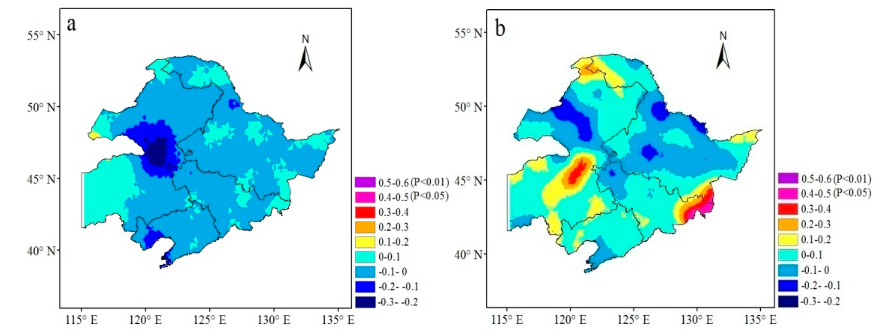
Figure 4.
Positions of points A, B, C, and D.

Figure 5.
Interannual variation in the burned area per year for northeast China as simulated by the uncalibrated LPJ-WHyMe model and the calibrated LPJ-WHyMe model and given by the GFEDv4. The numbers in brackets denote the time series correlations between the observations and simulations. (a): interannual variation in the burned area per year forpoint A; (b): interannual variation in the burned area per year forpoint B; (c): interannual variation in the burned area per year forpoint C; (d): interannual variation in the burned area per year forpoint D.

Figure 6.
Spatial distribution of the annual burned area averaged from 1997 to 2010 for the LPJ-WHyMe model with different parameter uncertainty ranges. (a): 25% parameter uncertainty range; (b): 50% parameter uncertainty range; and (c): 100% parameter uncertainty range. The spatial correlation coefficient (r) and mean absolute error (MAE) between the observations and simulations are also given.
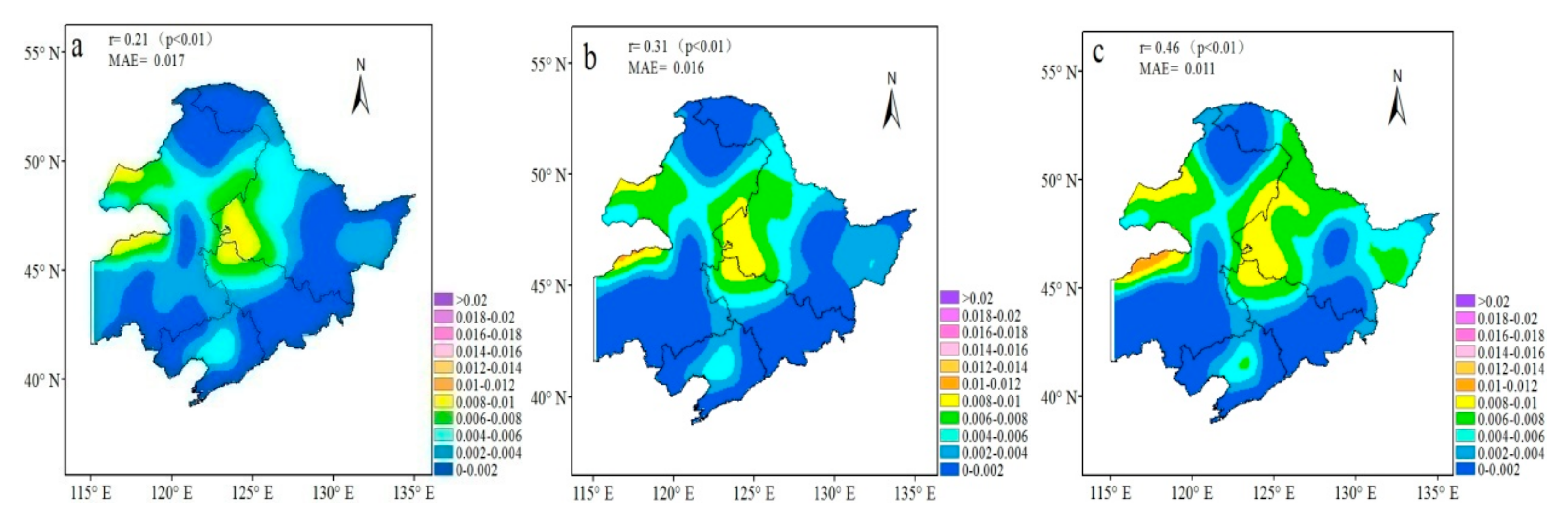
Figure 7.
Spatial distribution of the annual burned area averaged from 2011 to 2015 for the LPJ-WHyMe model with different parameter uncertainty ranges. (a): 25% parameter uncertainty range; (b): 50% parameter uncertainty range; and (c): 100% parameter uncertainty range. The spatial correlation coefficient (r) and mean absolute error (MAE) between the observations and simulations are also given.
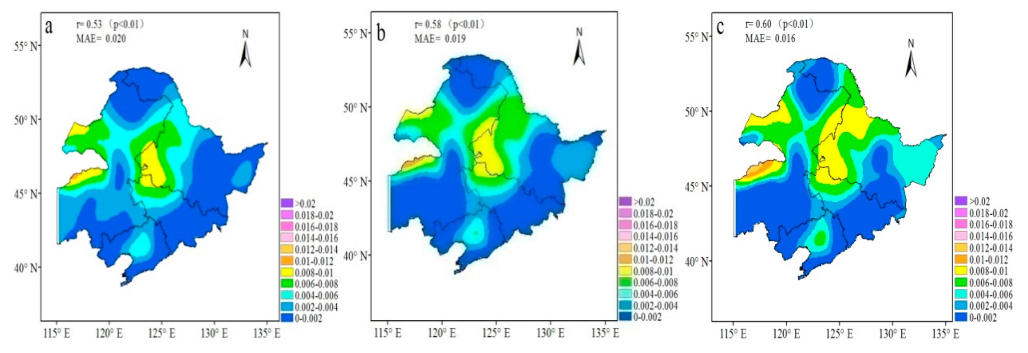
Figure 8.
Spatial distribution of the annual soil moisture (m3·m−3) averaged over the calibration period (1997–2010) and validation period (2011–2015).(a): soil moisturesimulated by the uncalibrated LPJ-WHyMe modelduring the calibration period; (b): soil moisturesimulated by the calibrated LPJ-WHyMe modelduring the calibration period;(c): soil moisturesimulated by the uncalibrated LPJ-WHyMe modelduring the validation period; (d): soil moisturesimulated by the calibrated LPJ-WHyMe modelduring the validation period.

Figure 9.
Spatial distribution of the annual total aboveground litter (g C·m−2) averaged over the calibration period (1997–2010) and validation period (2011–2015).(a): total aboveground littersimulated by the uncalibrated LPJ-WHyMe modelduring the calibration period; (b): total aboveground littersimulated by the calibrated LPJ-WHyMe modelduring the calibration period; (c): total aboveground littersimulated by the uncalibrated LPJ-WHyMe modelduring the validation period; (d): total aboveground littersimulated by the calibrated LPJ-WHyMe modelduring the validation period.


Table 1.
Chosen parameters within the LPJ-WHyMe model.
| Number | Parameter | Standard | Minimum | Maximum | Description |
|---|---|---|---|---|---|
| 1 | 0.7 | 0.2 | 0.996 | Co-limitation shape parameter | |
| 2 | 0.5 | 0.3 | 0.7 | Fraction of PAR assimilated at ecosystem level relative to leaf level | |
| 3 | 0.7 | 0.6 | 0.8 | Optimal ci = ca for C3 plants (all PFTs except TrH) | |
| 4 | 0.08 | 0.02 | 0.125 | Intrinsic quantum efficiency of CO2 uptake in C3 plants | |
| 5 | 0.015 | 0.01 | 0.021 | Leaf respiration as a fraction of Rubisco capacity in C3 plants | |
| 6 | 1.2 | 1.1 | 1.3 | q10 for temperature-sensitive parameter ko | |
| 7 | 2.1 | 1.9 | 2.3 | q10 for temperature-sensitive parameter kc | |
| 8 | 0.57 | 0.47 | 0.67 | q10 for temperature-sensitive parameter tau | |
| 9 | 0.25 | 0.15 | 0.4 | Growth respiration per unit NPP | |
| 10 | 3.26 | 2.5 | 18.5 | Maximum canopy conductance analog [mm·day−1] | |
| 11 | 1.391 | 1.1 | 1.5 | Evapotranspiration parameter | |
| 12 | 100 | 75 | 125 | Crown area = kallom1 * height ** krp | |
| 13 | 40 | 30 | 50 | Height = kallom2 * diameter ** kallom3 | |
| 14 | 0.67 | 0.5 | 0.8 | Height = kallom2 * diameter ** kallom3 | |
| 15 | 6000 | 2000 | 8000 | Leaf-to-sapwood area ratio | |
| 16 | 1.5 | 1.37 | 1.6 | Crown area = kallom1 * height ** krp | |
| 17 | 0.01 | 0.005 | 0.1 | Asymptotic maximum mortality rate [year−1] | |
| 18 | 0.4 | 0.2 | 0.5 | Growth efficiency mortality scalar | |
| 19 | 0.24 | 0.05 | 0.48 | Maximum sapling establishment rate [m−2·year−1] | |
| 20 | 7.15 | 6.85 | 7.45 | Leaf N concentration (mg·g−1) not involved in photosynthesis | |
| 21 | 200 | 180 | 220 | Specific wood density [kg C·m−3] | |
| 22 | 0.35 | 0.19 | 0.81 | Litter turnover time at 10 °C [year] | |
| 23 | 1.32 | 1.12 | 1.52 | Priestley-Taylor coefficient | |
| 24 | 0.17 | 0.15 | 0.19 | Global average short-wave albedo | |
| 25 | 2.00 | 1.80 | 2.20 | variables in percolation equation | |
| 26 | 0.9 | 0.6 | 1.0 | Fraction of active fraction of roots uptaking water from top soil layer | |
| 27 | 0.02 | 0.005 | 0.08 | LAI parameter, interception storage parameter | |
| 28 | 0.3 | 0.15 | 0.4 | Flammability threshold |
* means multiplication and ** means involution.
Table 2.
Parameter sensitivity analysis.
| Parameter Sensitivity Analysis | Parameter Uncertainty Range |
|---|---|
| 25% parameter uncertainty range | (standard − 0.25e1, standard + 0.25e2) |
| 50% parameter uncertainty range | (standard − 0.5e1, standard + 0.5e2) |
| 100% parameter uncertainty range | (standard − e1, standard + e2) |
© 2019 by the authors. Licensee MDPI, Basel, Switzerland. This article is an open access article distributed under the terms and conditions of the Creative Commons Attribution (CC BY) license (http://creativecommons.org/licenses/by/4.0/).
Share and Cite
MDPI and ACS Style
Yue, D.; Zhang, J.; Sun, G.; Han, S. Calibration and Assessment of Burned Area Simulation Capability of the LPJ-WHyMe Model in Northeast China. Forests 2019, 10, 992. https://doi.org/10.3390/f10110992
AMA Style
Yue D, Zhang J, Sun G, Han S. Calibration and Assessment of Burned Area Simulation Capability of the LPJ-WHyMe Model in Northeast China. Forests. 2019; 10(11):992. https://doi.org/10.3390/f10110992
Chicago/Turabian StyleYue, Dandan, Junhui Zhang, Guodong Sun, and Shijie Han. 2019. "Calibration and Assessment of Burned Area Simulation Capability of the LPJ-WHyMe Model in Northeast China" Forests 10, no. 11: 992. https://doi.org/10.3390/f10110992
Note that from the first issue of 2016, this journal uses article numbers instead of page numbers. See further details here.