Article

Improving Estimation Accuracy of Growing Stock by Multi-Frequency SAR and Multi-Spectral Data over Iran’s Heterogeneously-Structured Broadleaf Hyrcanian Forests

1
Department of Photogrammetry and Remote Sensing, Faculty of Geodesy and Geomatics Engineering, K, N. Toosi University of Technology, P.O.Box 15433-19967 Tehran, Iran
2
Department of Remote Sensing, University of Würzburg, Oswald KülpeWeg 86, 97074 Würzburg, Germany
3
Department of Forestry, University of Guilan, Entezam Square, P.O.Box 43619-96196 Some’e Sara, Iran
*
Authors to whom correspondence should be addressed.
Forests 2019, 10(8), 641; https://doi.org/10.3390/f10080641
Submission received: 26 June 2019 / Revised: 17 July 2019 / Accepted: 25 July 2019 / Published: 29 July 2019

Abstract

:
Via providing various ecosystem services, the old-growth Hyrcanian forests play a crucial role in the environment and anthropogenic aspects of Iran and beyond. The amount of growing stock volume (GSV) is a forest biophysical parameter with great importance in issues like economy, environmental protection, and adaptation to climate change. Thus, accurate and unbiased estimation of GSV is also crucial to be pursued across the Hyrcanian. Our goal was to investigate the potential of ALOS-2 and Sentinel-1’s polarimetric features in combination with Sentinel-2 multi-spectral features for the GSV estimation in a portion of heterogeneously-structured and mountainous Hyrcanian forests. We used five different kernels by the support vector regression (nu-SVR) for the GSV estimation. Because each kernel differently models the parameters, we separately selected features for each kernel by a binary genetic algorithm (GA). We simultaneously optimized R2 and RMSE in a suggested GA fitness function. We calculated R2, RMSE to evaluate the models. We additionally calculated the standard deviation of validation metrics to estimate the model’s stability. Also for models over-fitting or under-fitting analysis, we used mean difference (MD) index. The results suggested the use of polynomial kernel as the final model. Despite multiple methodical challenges raised from the composition and structure of the study site, we conclude that the combined use of polarimetric features (both dual and full) with spectral bands and indices can improve the GSV estimation over mixed broadleaf forests. This was partially supported by the use of proposed evaluation criterion within the GA, which helped to avoid the curse of dimensionality for the applied SVR and lowest over estimation or under estimation.

1. Introduction

Hyrcanian forests are known as remnants of the Pleistocene era that survived the frost period [1]. These forests are located in regions of northern Iran and part of Caucasus, and embrace a high species and structural diversity of uneven-aged mountainous broadleaf forests distributed across a high altitudinal gradient [1,2]. Recently, portions of these forests were inscribed in the list of UNESCO World Natural Heritages [3]. The growing stock volume (GSV) is one of the important allometric biophysical forest attributes. It is closely related to other forest quantities such as height and aboveground biomass and is of great importance in the forest ecology, management, and carbon storage [4,5]. Tree-level biomass is conventionally derived by using species-specific allometric relations and wood density from ground-based measurements. However, the high cost, time, and the limited geographical coverage prohibitively challenge these methods. On the other hand, remote sensing data from spaceborne SAR and multispectral sensors with proper radiometric and spatial resolution and sufficient time intervals of data acquisition from the desired areas have been proven to provide important proxies in forestry research [6,7]. Due to mentioned historical and environmental reasons, development and implementation of remote sensing-assisted methods serve the overarching aim of monitoring and sustainable management of Hyrcanian forests.
Amongst the recent attempts for GSV estimation by state-of-the-art multispectral data, Chrysafis et al. (2017) [8] estimated the GSV by blending the Sentinel-2 and the Landsat data with the Random Forest (RF) model, and concluded that near-infrared and the red edge domains greatly affect GSV estimation. In addition, Mura et al. (2018) [9] estimated the GSV by the Sentinel-2, Landsat, and the Rapideye sensors and concluded that, beside the near-infrared and red edge regions, the SWIR region is also effective because of its sensitivity to the water content in the canopy. In both studies Sentinel-2 data were suggested to excess others in performance.
The radio detection and ranging (radar) sensors considerably contributed to solving the limitations of optical sensors including their inability to penetrate the canopy and less sensitivity to the vertical canopy structure. The ability of radar data to estimate biophysical forest characteristics is also less susceptible to weather conditions and acquisition time, which eases monitoring of mountainous forests that mostly occur in humid, cloudy, and foggy areas. However, changes in radar wavelength and type of polarization results in differences in both analytical workflow and the achieved estimation performance. Moreover, higher trunk volume leads to underestimation of actual GSV values due to the saturation in the scattering form dense canopy, which improves with an increase in wavelength [10,11,12]. Gao et al. (2018) [13] estimated GSV by the Dual polarized ALOS-1 data and reported a higher potential and later saturation of L-band HV cross-polarization channel than HH co-polarized channel. By using multi-temporal dual polarized ALOS-1 sensor data, Antropov et al. (2013) [14] concluded that the multi-temporal method was superior in prediction (with HH co-polarized channel performing better for mature trees), yet the saturation happens in the high GSV values. In addition, Chowdhury et al. (2014) [15] estimated the GSV by the ALOS-1 multi-temporal full polarimetric data, from which covariance and coherency matrices, as well as the phase difference between HH & VV channel and the coherency between HH and VV channels, were extracted. They showed that full polarimetry data has a high ability for GSV estimation.
Multi-sensor remote sensing approaches are highly capable for forest applications. In our study, we percept GSV estimation over mountainous broadleaf forests from a slightly different perspective. The biophysical characteristics of forest can be studied in multi-spectral approach by focusing on the biochemical aspects such as chlorophyll and in SAR approach on radar wave penetration in the canopy [16,17]. Mauya et al. (2019) [18] estimated GSV by the ALOS-2’s global mosaic, the Sentinel-1 and the Sentinel-2 sensors data. They concluded that using SAR data alone was unlikely to provide a good estimation ability for GSV, while a combined use of Sentinel-1 and Sentinel-2 data were advantageous. In Iran’s Hyrcanian region, recent investigations of the ability of remotely sensed data and methods include Vafaei et al. (2018) [19] who estimated biomass by the ALOS-2 full polarimetric and Sentinel-2A data. The Sentinel-2 returned the moderate accuracy, whereas the ALOS-2 individually led to minimum estimation accuracy.
The overall objective of this research was to estimate the GSV in Hyrcanian uneven-aged mountainous broadleaf forests based on leveraging a broad range of possibilities in optical and radar data processing. To this aim, we used ALOS-2 full polarimetric, Sentinel-1 dual polarimetric and Sentinel-2 multi-spectral data. We only concentrated on combined use of polarimetric and spectral features. In addition, we compared five different kernels in support vector regression (SVR) for GSV estimation. We additionally applied a heuristic feature selection by binary genetic algorithm, in which we simultaneously optimized the root mean square error (RMSE) and coefficient of determination (R2) for each kernel separately. The workflow and findings of this study are mainly significant due to multiple challenges associated with the structure and composition of our test site, including the severe topography, limited field samples, highly mixed tree species in various ages, and complex slope-aspect structure.

2. Materials and Methods

2.1. Study Area

The study area is located in Guilan province’s Nav-Asalem region in northern Iran (see Figure 1). The altitude varies between 100 to 2000 m above sea level, and the slope ranges from 0 to 73 degrees. The climate is temperate and cold, average annual rainfall is 1200 mm per year and the mean temperature is 12.4-degrees Celsius. The forest comprises uneven-aged mountainous broadleaf stands dominated by oriental Beech (Fagus orientalis Lipsky.) and hornbeam (Carpinus Betulus L.), accompanied by other broadleaf shrub and tree species.

2.2. Field Data Inventory

Field data were collected during July 2014 to March 2015. The in situ measurements were conducted in 148 circular plots with 18 m radius each and distributed in a randomly positioned square grid, as prescribed by the technical bureau of the Iranian Forests, Rangelands and Watershed Management Organization (FRWO) [20]. In each plot, the diameter at breast height (DBH; i.e., 1.5 m above ground surface) and the species type were recorded for all trees. For a sample of trees, the dominant species was recorded in each plot. Finally, the GSV values were calculated in each stand by means of DBH and lookup tables for each species separately.
Plot center locations were collected by global positioning system (GPS) in the WGS84 coordinate system. The original values of GSV in each plot were multiplied by 10 in order to be transformed from m3 per 0.1 hectares to m3 per hectare. The inventoried GSV ranged between 98.60 and 385.8 m3 ha−1 (see Table 1).

2.3. Remotely Sensed Data

2.3.1. Sentinel-2 Data

Sentinel-2 satellite carries a multi-spectral sensor in 13 bands from 400 nm to 2400 nm with spatial resolutions of 10, 20, and 60 m [21]. The 60-m resolution bands include B1 (430 nm), B9 (940 nm) and B10 (1340 nm) that are mainly used for atmospheric correction. The Sentinel-2 data in Level1C was acquired on 21 June 2016 and downloaded from European Space Agency (ESA) repository. After performing the atmospheric and geometric correction incorporating SRTM 1 aSec DEM [22], the spectral features were extracted from Sentinel-2 data. Since the acquired Level1C data represents the top-of-atmosphere (TOA) reflectance, we used Sen2Cor algorithm for atmospheric correction to calculate Level 2A data representing the bottom-of-atmosphere (BOA) reflectance. The sen2cor algorithm is an image-based correction that performs image correction based on lookup tables extracted from RadTran algorithm [23], with the main benefit that it does not need local meteorological data for correction. We only used the original bands and vegetation indices (see Table 2) for GSV estimation. Due to the different spatial resolutions of the Sentinel-2 imagery, we used the 5 × 5 local window for bands and indices with 10 m spatial resolution, whereas 3 × 3 local window was used for bands and indices with 20 m spatial resolution. The mean values of data extracted in each local window over each field plot inventory were applied for GSV estimation. The entire process was performed in SNAP V6 software [24].

2.3.2. Sentinel-1 Data

Sentinel-1 is equipped with a synthetic aperture radar (SAR) antenna that scans the Earth in dual polarization mode in VV and VH channels in the C band. Our study area was scanned in dual polarization mode on 22nd of July 2017 and data was downloaded from the ESA repository. The data was scanned in single look complex (SLC) mode using the interferometric wide (IW) method. The dataset was primarily calibrated. Since the data was in dual polarimetry mode, the calibration was performed in the complex calibration manner to preserve the phase information. For extracting polarimetric information, we first extracted the C2 matrix (non-coherent covariance matrix) from the calibrated data. For dual polarimetric data, we used the Equation (1) to calculate the C2 matrix [40]. Data was scanned by IW method and was thus required to be debursted by the Sentinel-1 TOPS deburst method. For squared pixels, we applied the multi-looking operator with five looks in the azimuth direction and one look in the range direction to reach the 17-meter resolution, i.e., the spatial resolution close to the field sample plot size. For protecting polarimetric information, we applied the polarimetric refined Lee filter (7 × 7 local window) on the debursted C2 matrix to decrease the speckle noise [39]. The range-doppler terrain correction method with the SRTM 1Sec HGT DEM [22] was used to georeference the C2 matrix. Finally, the dual-polarimetric H-A-Alpha decomposition was applied on the georeferenced C2 matrix [40]. Consequently, we used a 3 × 3 local window due to the available 17 m spatial resolution to extract information on sample plot level. The entire analysis was performed in SNAP V6 software [24]. The extracted features are summarized in Table 3.
C 2 = [ | S V V | 2 S V V S V H * S V H S V V * | S V H | 2 ]

2.3.3. ALOS-2 PalSar Data

The ALOS-2 satellite features a fully polarimetric synthetic aperture radar (SAR) antenna. This sensor scans the Earth in HH, HV, VH, and VV polarization channel in L band. We downloaded the data acquired on 10th of June 2015 over our study site from the repository provided by the Japan Aerospace Exploration Agency (JAXA). This data was scanned in SLC mode with Stripmap-2 method. The data preprocessing was performed solely for the polarimetric features. For preserving phase information, the raw data was initially calibrated in the complex calibration manner. The T3 coherency matrix was extracted from the calibrated data (Equation (2)) [41]. One may note the negative effects caused by the severe topography on scattering from the scatterers and consequently on the polarimetric information [42]. One crucial effect of topography is the rotation of radar wave in the line of sight because of the slope in the azimuth direction. This phenomenon is known as polarization orientation angle (POA) and is compensated by applying Equations (3)–(5) [41,42,43]. The multi-looking operator with six looks in azimuth direction and four looks in range direction was applied to the T3 matrix for the squared pixel and speckle noise reduction. Finally, we reached the 15-m spatial resolution that was close to those of field sample plots. As already mentioned for Sentinel-1 data processing, we used refined Lee speckle filter to simultaneously reduce speckle noise and preserve polarimetric information [41,44,45]. The filter was applied with 7 × 7 local window, 3 × 3 target window, and sigma of 0.9 to the T3 matrix. Following these steps, the T3 matrix was consequently georeferenced by SRTM 1Sec HGT DEM [22] using the range-doppler terrain correction method. In this research, we only extracted the polarimetric features (see Table 4). We used a 3 × 3 local window to extract the information on sample plot level. Similar to the preceding steps, the processes were performed in SNAP V6 [24].
S = [ S H H S H V S V H S V V ] . k = 1 2 [ S H H + S V V S H H S V V 2 S H V ]   . T 3 = k k * T
δ = 1 4 [ tan 1 ( 4 R e ( ( S H H S V V ) S H V * ) | S H H S V V | 2 + 4 | S H V | 2 ) + π ]
V = 1 2 [ 1 + cos 2 δ 2 sin 2 δ 1 cos 2 δ 2 sin 2 δ 2 cos 2 δ 2 sin 2 δ 1 cos 2 δ 2 sin 2 δ 1 + cos 2 δ ]
T 3 P O A = V T 3 V T
In the equations S is the stocke’s matrix, SHH to SVV are the four polarizations, k is the Pauli target vector for calculating T3 matrix, and δ is the POA angle.

2.4. Modeling by Machine Learning

2.4.1. Support Vector Regression

Support vector machine (SVM) is known as powerful, flexible, and robust-to-noise machine learning method. The main goal of SVM is to minimize the sum of squares error (SSE) in Equation (6) during the model training procedure. The support vector regression (SVR) is a regression version of SVM [50,51]. There are two main methods for SVR, ε and υ regression. In ε regression, an insensitive tube defines by ε parameter, but this parameter is user-defined and the procedure affects model accuracy by only involving noisy observation in the big values of ε or the non-important observation data in the small values of ε, which results in non-generalized model that cannot model different behaviors of the phenomena [50,52,53]. In the υ regression method, the υ parameter defines the fraction of support vectors number involved in the modeling procedure [52]. In this method, the ε is automatically calculated in the algorithm and better controls support vectors. Therefore, both caveats of the ε method including challenge of the selection of proper ε value and its effect on accuracy could be resolved [52]. Therefore, we used the υ regression. The kernel based solution was used for accommodating the non-linear and complex behaviors. The used kernel passes the features into a new feature space [53], following which the model is trained in the new feature problem [51]. Whereas there are various kernels for SVR, the choice proper kernel for each problem depends on the nature of the problem [49]. We tested five different kernels (see Table 5). We tuned the hyper-parameters by repeated cross-validation based on RMSE (see Section 2.4.3). Besides the kernel’s hyper-parameter, the cost parameter was also tuned with each kernel to maintain the model’s flexibility [51].
min ( 1 2 w 2 + C ( ν ε + 1 l i = 1 l ( ξ i + ξ i * ) ) )
In Equation (6), C regularization constant, υ parameter between 0 and 1, ε value and ξ i * is slack variable. We analyzed the results of three different experiments. In the first experiment, the GSV was modeled using a single sensor approach. In the second experiment, we modeled the GSV using all the features obtained through the multi-sensor approach. Finally, in the third experiment, we model the GSV using the GA selected features.

2.4.2. Feature Selection

Feature selection is an essential task in working with hyper-dimensional data, in which the best subset from all features is selected based on lower cost of model training and higher accuracy. This solution is essential in the presence of a large number of extracted features and small sample size to avoid the prohibitive effects of the curse of dimensionality on model performance and interpretability [55]. Therefore, a proper method for feature selection cares for the low training cost while avoiding the curse of dimensionality in the modeling [56]. The genetic algorithm (GA) is an evolutionary method for optimization. The method is inspired by natural selection in the real world, with the main idea of incorporating a wide range of suitable solutions that leads to selection of an optimum solution [57]. We used binary GA for feature selection. First, a population of chromosomes with 0 and 1 genes was randomly generated in which each chromosome is considered as a solution. The goodness of each solution was determined by the fitness function. The solutions with higher goodness had a higher chance to create a new solution. The new solution was then created by crossover procedure from two randomly selected solution with a high fitness value. The mutation operator changed the random genes with little probability and was used to maintain genetic diversity from one generation of a population of genetic algorithm chromosomes to the next. Finally, the algorithm was iterated until the fitness value remained unchanged [58]. Here, we selected the features for each kernel individually by cross-validation (see Section 2.4.3). The fitness function pursued the goal to simultaneously RMSE and R2 values (see Figure 2). For this purpose, the fitness function as defined in Equations (7)–(9) was proposed. In this fitness function, the highest fitness value could potentially occur in R2 equal to 1 and RMSE equal to 0, i.e., a fitness value equal to 190.
α = 90 tan 1 ( R M S E 100 × R 2 )
d = R M S E 2 + ( 100 × R 2 ) 2
f i t n e s s = α + d

2.4.3. Validation

The validation of model performance is the essential step in modeling [20]. Due to the most common case of limited sample size, using the k-fold cross-validation was necessary to avoid noisy and unstable predictions [18,50]. The RMSE, R2 (Equations (10)–(11)) were used as error diagnostics based on their proven usefulness in assessing prediction of forest parameters [18,59]. In addition, the model stability in the presence of limited field sample size was checked by the repeated k-fold cross-validation. The model was assessed as more stable if the standard deviation (Equation (13)) of each of the diagnostic metrics was closer to zero [60]. Also we used MD (see Equation (12) for models over-estimation or under-estimation analysis. The higher positive values indicates the over-fitting and higher negative values indicates the under-fitting problem [61]. We used the 5-fold cross validation with 20 repetitions for more stable feature selection in the GA (Section 2.4.2), kernel’s hyper-parameter tuning (Section 2.4.1) and finally, the model validation. The statistical modeling and the feature selections were implemented in open source domain in R using the kernlab, caret, and GA libraries.
R M S E = i = 1 n ( y i o b s y i p r e d ) 2 / n
R 2 = i = 1 n ( y i p r e d y ¯ ) 2 / i = 1 n ( y i o b s y ¯ ) 2
M D = 1 n i = 1 n ( y i p r e d y i o b s )
S D = i = 1 m ( P i P ¯ ) 2 / m
In the Equations, the y i o b s is the observed GSV in plot i, y i p r e d is the predicted GSV, n is the number of samples in fold, y ¯ is the GSV’s average in fold, P i is the validation metric in each fold, P ¯ is the metric’s average and m is the number by which the model was trained with different data.

3. Results

3.1. Single Sensor Models

3.1.1. Sentinel-2

Here, the 31 features extracted from the Sentinel-2 data were used for the GSV modeling (see Table 2). As previously mentioned in Section 2.3, the SVR model was employed using five different Kernels. The kernel’s hyper-parameters were tuned with repeated cross-validation. The results can be seen in Table 6.
As can be seen in Table 6, from the perspective of performance, the Bessel kernel with RMSE = 31.536 and R2 =0.676 provided a better performance compared to other kernels. The polynomial kernel presented a very close performance to the Bessel Kernel. From the perspective of model stability (see Section 2.3.3), the Polynomial kernel with RMSE_SD = 2.630 and R2_SD = 0.071, provided more stable results than other kernels. The RBF kernel was the second more stable kernel (Table 6). The MD index shows that the all models are under estimate the GSV.
By considering both the models performance, stability and MD analysis the polynomial kernel exceeded other kernels, while all models generally showed close performance. Finally, no significant difference was observed amongst the kernels in the GSV modeling using the features extracted from Sentinel-2 (see Figure 3, Figure 4 and Figure 5).

3.1.2. ALOS-2

Here, 45 features were extracted from ALOS-2 data (see Table 4). The results are shown in Table 7.
As shown in Table 7, the sigmoid kernel with provided a better performance compared to other kernels by returning RMSE = 46.086 and R2 = 0.327. This was closely followed by the RBF kernel with RMSE = 46.588 and R2 = 0.318. Concerning the stability, the RBF kernel was more stable than other kernels (RMSE_SD = 6.510 and R2_SD = 0.123), followed by Bessel kernel. The Laplace kernel showed similar stability to that of Bessel kernel, yet a considerably lower performance compared with other kernels (see Table 7). The MD index shows that all of models significantly over estimate the GSV.
By considering both performance and stability and MD analysis, the RBF provided better results compared to the other kernels. However, all kernels performed roughly close to each other, with no significant difference between the kernels in the GSV modeling using the ALOS-2 features (see Figure 3, Figure 4 and Figure 5).

3.1.3. Sentinel-1

In this experiment, seven features, extracted from Sentinel-1 data solely were used for the GSV modeling (see Table 3). The results are show in Table 8.
As can be seen in Table 8, the Laplace kernel exceeded all other applied kernels with RMSE = 46.815 and R2 = 0.299 again, closely followed by the Bessel kernel with RMSE = 46.879 and R2 = 0.297. Moreover, the Bessel kernel provided more stable results than other kernels (RMSE_SD = 6.302 and R2_SD = 0.113). The MD index shows that all of models significantly over estimate the GSV after ALOS2. By considering both performance and stability, the Bessel kernel was slightly better compared to the other kernels.

3.2. Multi-Sensor Models

Here, we employed 83 features, obtained from Sentinel-2, ALOS-2, and Sentinel-1 data (see Table 2, Table 3 and Table 4). The results are shown in Table 9.
The sigmoid kernel performed best (RMSE = 32.636 and R2 = 0.659), followed by polynomial kernel (RMSE = 32.682 and R2 = 0.659). In addition the sigmoid kernel resulted in the most stable model with RMSE_SD = 2.905 and R2_SD = 0.067. The MD index shows that all of models except Bessel moderately under estimate the GSV.
As can be observed in Figure 3, Figure 4 and Figure 5, stacking the entire features into one feature set did not improve the results. This is mainly due to the joint effect caused by the curse of dimensionality and the limited sample size, and suggests the necessity of feature selection as an essential task.

3.3. Multi-Sensor Approach with Selected Feature

The Table 10 summarizes the results of models built with features optimized using the binary genetic algorithm as described in Section 2.4.2.
The Laplace kernel provided a superior predictive accuracy to other kernels. This was followed by the polynomial kernel. However, the RBF kernel proved to return the most stable predictions, followed by the polynomial kernel.
All in all, the highest accuracies for GSV prediction were returned by the polynomial kernel. Table 11 summarizes the range of various features selected for the GSV modeling using each kernel. The selected features mainly include the ALOS-2 polarimetric decomposition, Sentinel-1 H-A-Alpha decomposition, and Sentinel-2 spectral features including NIR, red edge, SWIR bands and vegetation indices. The proper feature selection which resulted in the parsimonious feature sets enables achieving both predictive accuracy and model stability and robustness. Also, the MD index for all of the models compared to other experiments approach zero, especially for the polynomial kernel (MD = −0.041).
As summarized in Figure 3, Figure 4 and Figure 5 the performance of multi-sensor approach with selected features was slightly better than that achieved by Sentinel-2, which suggest that including selected polarimetry features along with the multi-spectral information improves the GSV across mountainous broadleaf stands. Also the over estimation or under estimation problem was solved in this experiment. For polynomial kernel the MD is equal to −0.041 and it is best MD index between all of experiments.

4. Discussion

The main objective of this research was to estimate the GSV in heterogeneously-structured and mountainous Hyrcanian forests in northern Iran. Predictive models and continuous monitoring of forest are especially vital in Iran’s Hyrcanian forests because of the current ongoing rate of degradation and their crucial role in Iran’s Hyrcanian forest ecosystem. Thus, investigating the potential of multi-frequency SAR, multi-spectral optical data for generating the reliable predictive models are essential in this study area. In this research, the GSV modeling was carried out using the polarimetric and multi-spectral features and their combination using three different approaches. The SVR with five various kernels was used for modeling because of non-linear and complex relation of features with the GSV particularly in multi-sensor approach. Also, there were several challenges in this procedure including the severe topography, limited field samples, highly mixed tree species in various ages, and complex slope-aspect structure.
In the first experiment, the GSV was modeled using the Sentinel-2 multi-spectral features. B11 and B12 bands from SWIR spectral region showed a high contribution because of their sensitivity to the water content in the canopy, that confirmed in research by Chrysafis et al. (2017) [8] and Mura et al. (2018) [9]. We also found the NIR and the red edge bands as good features in modeling which is due to their sensitivity to the chlorophyll and pigments of tree leaf. Relevant works of Chrysafis et al. (2017) [8], Mura et al. (2018) [9], and Chrysafis et al. (2019) [62] also described these features as influential features for the GSV estimation in their research. Basically, the vegetation indices that use the NIR and red-edge spectral bands have an effective contribution in the GSV estimation. This is mainly because of that the VI uses the combination of spectral bands and reaches the information that cannot be extracted from the single spectral band, as Chrysafis et al. (2017) [8] found this in their research. The Mura et al. (2018) [9] and Chrysafis et al. (2019) [62] also found that VIs have an effective contribution to GSV estimation.
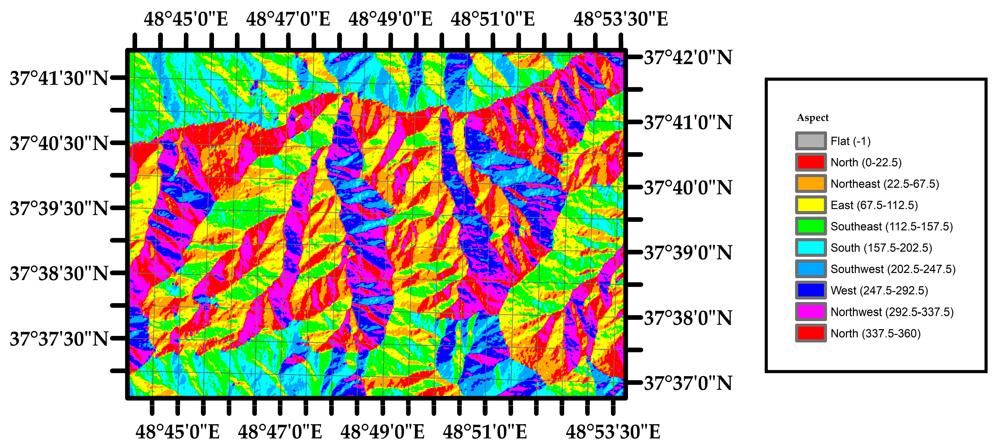
The performed analysis indicated that the GSV modeling with ALOS-2 polarimetric features produced non-satisfactory results. However, increasing the number of polarimetric features can improve the results. The two main challenges for GSV modeling with ALOS-2 data in this study area are the harsh topography and the limited number of field inventory samples. As shown in Figure 6, the study area embrace harsh mountainous forest stands with high elevational gradient and complex slope-aspect structure. In this type of topography, phenomena like shadow and layover occur in SAR data. Particularly, no scanned data from the study areas were found for shadowing. Nevertheless, the radiometric values were significantly affected in layover behavior. Another effect is the POA (see Section 2.3.3) which was compensated in the preprocessing steps and thus results in no notable problem for the GSV modeling [43]. Yet the effect of slope in range direction, known as angular variation effect (AVE), still remains. In areas with forest cover and longer radar wavelength, the AVE introduces a notable effect. As such the double scattering mechanism increases in the slopes that face the radar incoming wave, whereas it decreases in opposite slopes. In addition, the volume scattering mechanism increases since the severe topography causes an increase in cross-pol scattering. In a severe mountainous area like our research site, the proposed correction methods do not completely refine the results [42,63]. In addition, a further effect is the effective scattering area due to the non-homomorphic imagining of radar. This effect can be maximized in the mountainous areas and thus dramatically affect the geo-referencing of the applied SAR data. This effect causes the higher radiometric values in front slopes facing the incoming radar wave and lower radiometric values in opposite slopes [42,43,63].
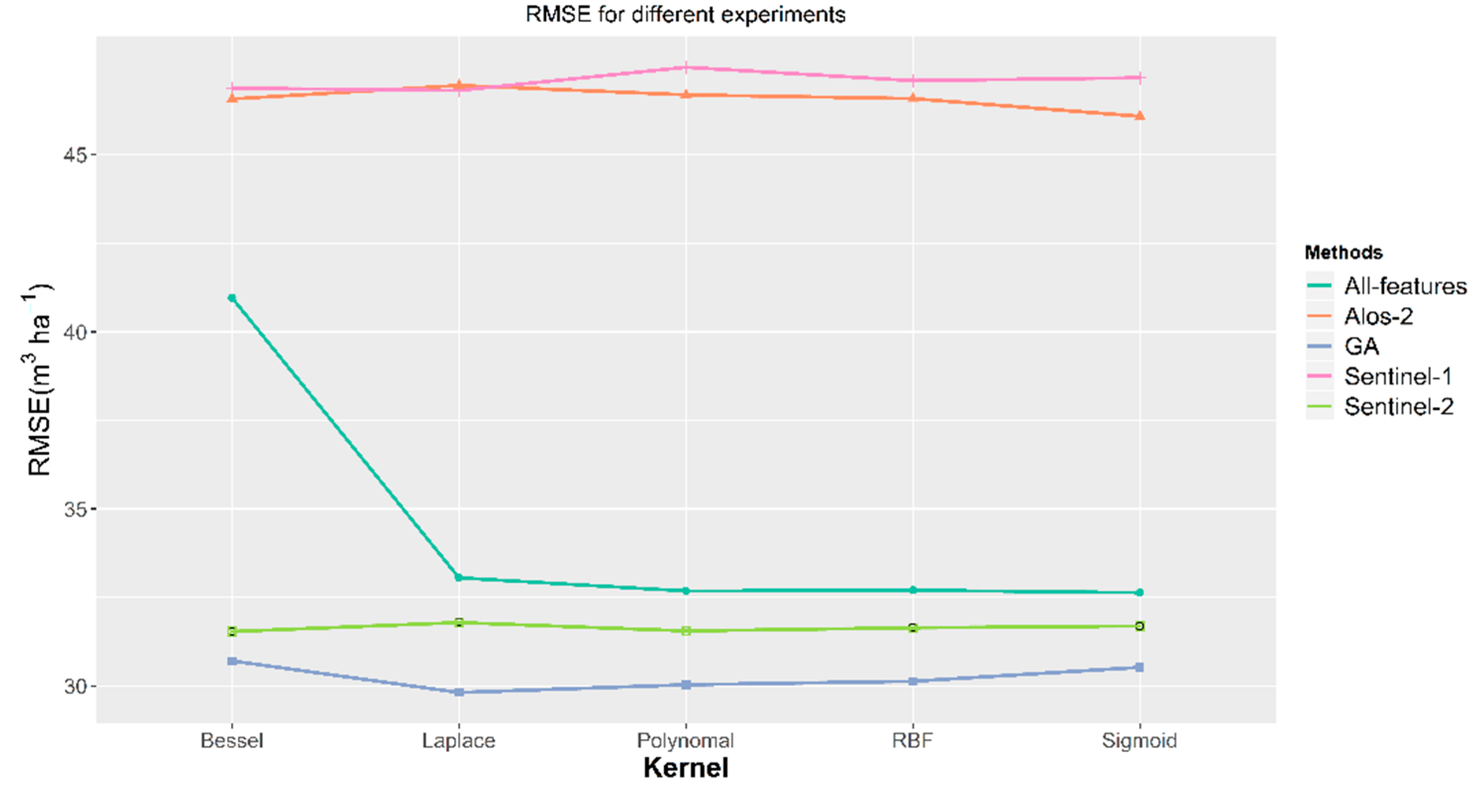
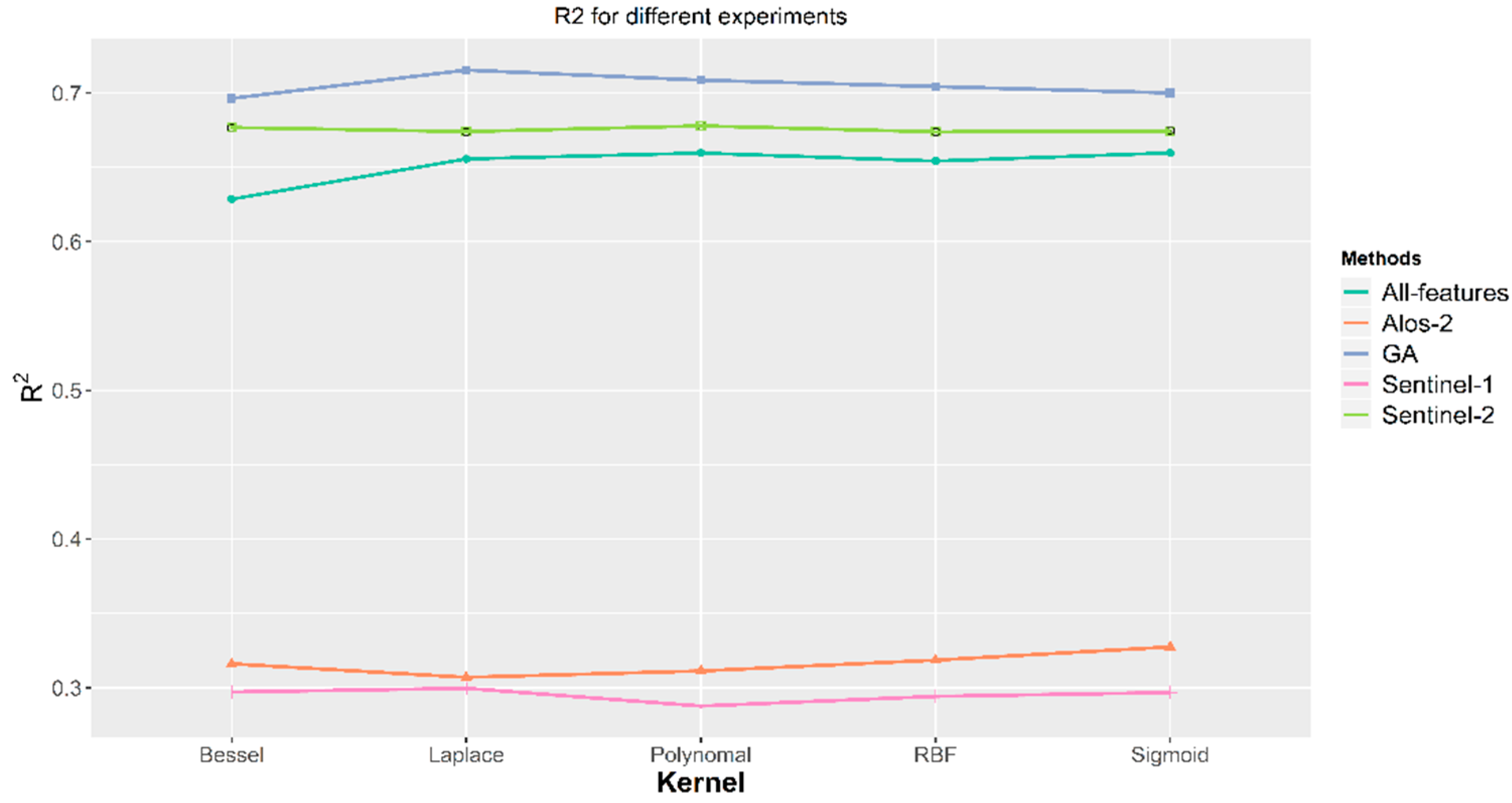
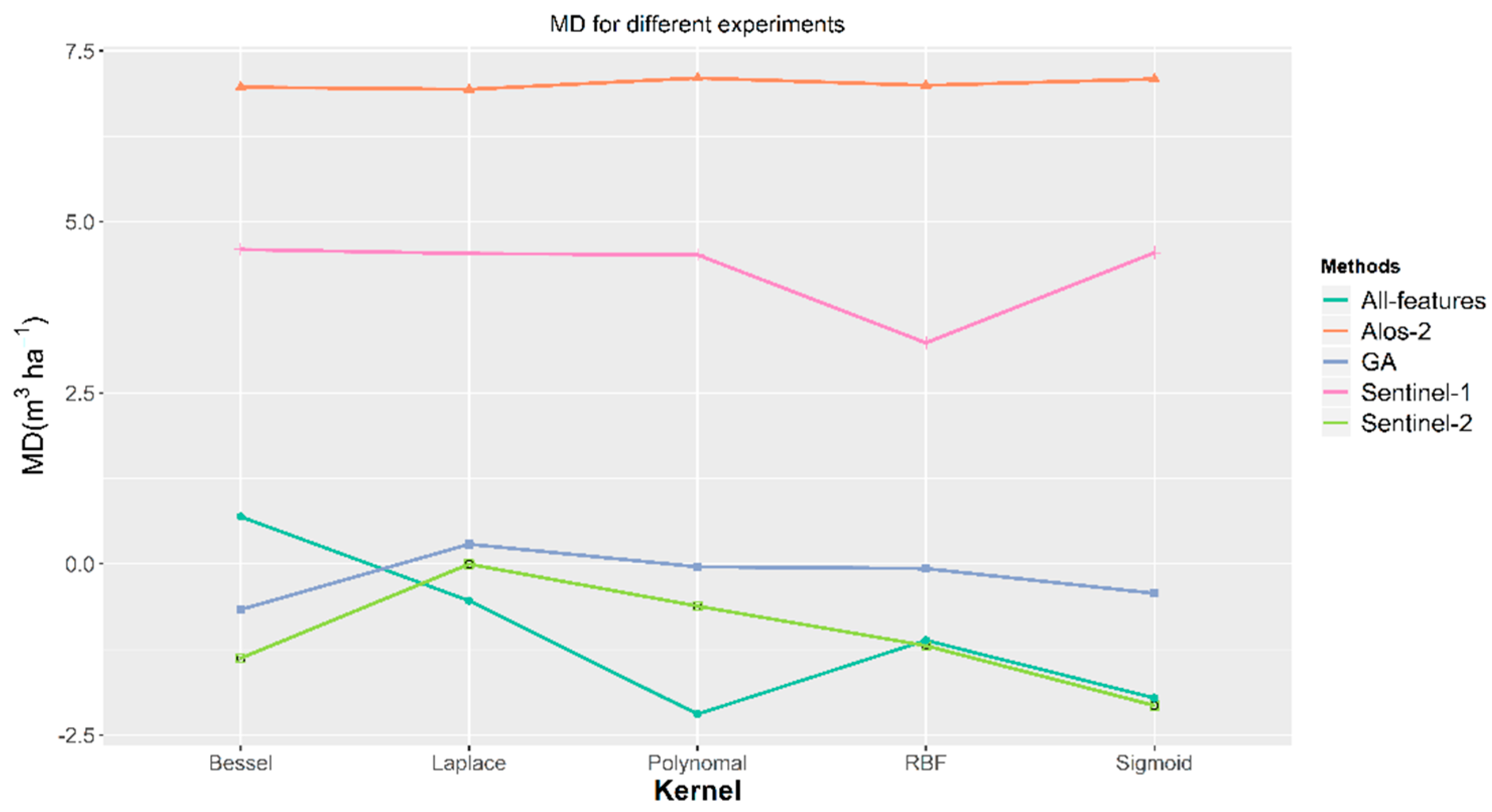
The second challenge for modeling GSV is caused by limited number of field inventory samples that is commonly the case across heterogeneously-structured uneven-aged Hyrcanian forests. Apart from statistical and model-related problems, this particularly hindered us from building species-specific GSV models and thus considering differences in scattering from tree species or different age classes. The collective effects of the above mentioned issues led to the rather mediocre results obtained by ALOS-2 data in our study (see Figure 3, Figure 4 and Figure 5). The H-A-Alpha decomposition features have an average ability in the GSV estimation. Vafaei et al. (2018) [19] found that these features have an average ability for biomass estimation in Hyrcanian forests too. The Touzi decomposition’s features are also effective, Sharifi et al. (2015) [64] found that the Tozi decomposition describes the target asymmetry in the forested area and can use for biomass estimation in Hyrcanian forest. The Van Zyle, Cloude, and Freeman decomposition features based on volume or double mechanism are effective in GSV modeling because of L-band wavelength penetration in the canopy and interaction with the tree’s stem and ground. So they are reasonable features for the GSV modeling as Kumar et al. (2012) [65] found this behavior. The achieved performance and model stability are comparable to similar research. Compared with the only available relevant case study from the area, Vafaei et al. (2018) [19] used limited polarimetry features. Unlike their study, we extracted a large number of polarimetric features in our research. Especially comparing to Vafaei et al. (2018) [19] with ALOS-2 in the same region, his conclusion is that ALOS-2 has a very weak ability for biomass estimation (R2 = 16%). Since the biomass and GSV have near relation [5], we greatly improved the prediction ability for GSV with different target decomposition features (R2 = 32%).
The performed analysis indicated that the modeling with Sentinel-1 polarimetric features produced non-satisfactory results for GSV modeling. The Sentinel-1 features are not frequently used in forestry research because of the shorter wavelength (C-band) of the data. In this wavelength, the scattering only occurs in the upper part of the canopy. In our study, we applied the dual polarimetric H-A-Alpha decomposition. Our result has better performance (R2 = 29%) than Mauya et al. (2019) [18] who only used the scattering coefficient in GRD mode and achieved R2 = 18%. Therefore, we can conclude that using the Sentinel-1 dual polarimetry H-A-Alpha decomposition is useful for GSV estimation. As can be seen in Figure 3, Figure 4 and Figure 5, the results obtained by the Sentinel-1 data were inferior than those of Sentinel-2 and ALOS-2 data. In addition to the underlying reasons as referred earlier, one may also note the lower penetration rate of the C-band Sentinel-1 compared with the L-band ALOS-2. This will result in a lower sensitivity to biophysical parameters such as GSV.
Finally, the performed analysis on the multi-sensor approach indicated that the GSV modeling with all of the features did not enhance the results compared to the modeling by Sentinel-2. This is mainly due to the curse of dimensionality effect and the limited sample size. To deal with this problem, we modeled the GSV by multi-sensor approach using the selected features. The results indicated that the modeling with the selected features provide better results than the modeling by Sentinel-2. The features were selected for each kernel separately proper feature selection procedure provides a good and stable GSV modeling which is not suffering from the curse of dimensionality anymore. Also, the over-estimation or under-estimation was reduced greatly by our feature selection method (see Figure 5). As a result, the simultaneous integration of multi-spectral and radar data features produce satisfactory and stable models for GSV modeling compare to the Mauya et al. (2019) [18], Vafaei et al. (2018) [19], and Sharifi et al. (2015) [64] works. Due to the general novelty of in-depth and state-of-the-art remote sensing analysis over Hyrcanian forests. In future research, issues such as the effects of different topographic corrections for polarimetry data, forest species type mapping, novel SVR kernels, application of feature fusion, and texture features will be explored.

5. Conclusions

This study generated empirical evidence on the use of ALOS-2, Sentinel-2, and Sentinel-1remotely sensing data for GSV estimation in Iran’s Hyrcanian forests on a landscape scale. We used nu-SVR with five kernels for non-linear behavior modeling. The result showed that in single sensor approach only the Sentinel-2 returned better results, while shortcomings were observed when applying ALOS-2 and Sentinel-1 across heterogeneously-structured and mountainous Hyrcanian forests with limited field samples. In multi-sensor approach, the curse of dimensionality caused inferior results compared with the case of Sentinel-2. In addition, we tested selecting features in multi-sensor approach individually for each kernel by GA based on simultaneous optimization of diagnostic measures in a proposed fitness equation. This contributed to both higher performance and more model stability with the lowest underestimation.

Author Contributions

M.S.A., Y.M., H.L., and F.F. designed the research. F.F. provided field inventory sample data and advised the data analysis and interpretation. M.S.A. conducted data processing. M.S.A., Y.M., and H.L. analyzed the results. M.S.A. coded the statistical computation. M.S.A., Y.M., H.L., and F.F. wrote and commented the manuscript. H.L. and Y.M. were corresponding authors.

Funding

This research received no external funding.

Acknowledgments

We thank KNTU for technical support. We also thank ESA for providing open access Sentinel-1 and Sentinel-2 data. Also, JAXA is appreciated for providing ALOS-full polarimetry data via their data provision campaign.

Conflicts of Interest

The authors declare no conflict of interest.

References

  1. Ramezani, E.; Mohammad, R.; Mohadjer, M.R.M.; Knapp, K.-D.; Ahmadi, H.; Joosten, H. The late-Holocene vegetation history of the Central Caspian (Hyrcanian) forests of northern Iran. Holocene 2008, 18, 307–321. [Google Scholar] [CrossRef]
  2. Attarchi, S.; Gloaguen, R. Classifying complex mountainous forests with L-band SAR and landsat data integration: A comparison among different machine learning methods in the hyrcanian forest. Remote Sens. 2014, 6, 3624–3647. [Google Scholar] [CrossRef]
  3. United Nations Educational, Scientific and Cultural Organization (UNESCO), Hyrcanian Forests. Available online: https://whc.unesco.org/en/list/1584 (accessed on 5 July 2019).
  4. Somogyi, Z.; Teobaldelli, M.; Federici, S.; Matteucci, G.; Pagliari, V.; Grassi, G.; Seufert, G. Allometric biomass and carbon factors database. iForest Biogeosci. For. 2008, 1, 107–113. [Google Scholar] [CrossRef]
  5. West, P.W. Tree and Forest Measurement; Springer: New York, NY, USA, 2015. [Google Scholar]
  6. Yadav, B.K.V.; Nandy, S. Mapping aboveground woody biomass using forest inventory, remote sensing and geostatistical techniques. Environ. Monit. Assess. 2015, 187, 308. [Google Scholar] [CrossRef] [PubMed]
  7. Zhang, H.; Zhu, J.; Wang, C.; Lin, H.; Long, J.; Zhao, L.; Fu, H.; Liu, Z. Forest growing stock volume estimation in subtropical mountain areas using PALSAR-2 L-band PolSAR data. Forests 2019, 10, 276. [Google Scholar] [CrossRef]
  8. Chrysafis, I.; Mallinis, G.; Siachalou, S.; Patias, P. Assessing the relationships between growing stock volume and Sentinel-2 imagery in a Mediterranean forest ecosystem. Remote Sens. Lett. 2017, 8, 508–517. [Google Scholar] [CrossRef]
  9. Mura, M.; Bottalico, F.; Giannetti, F.; Bertani, R.; Giannini, R.; Mancini, M.; Orlandini, S.; Travaglini, D.; Chirivi, G. Exploiting the capabilities of the Sentinel-2 multi spectral instrument for predicting growing stock volume in forest ecosystems. Int. J. Appl. Earth Obs. Geoinf. 2018, 66, 126–134. [Google Scholar] [CrossRef]
  10. Askne, J.I.H.; Fransson, J.E.S.; Santoro, M.; Soja, M.J.; Ulander, L.M.H. Model-based biomass estimation of a hemi-boreal forest from multitemporal TanDEM-X acquisitions. Remote Sens. 2013, 5, 5574–5597. [Google Scholar] [CrossRef]
  11. Bharadwaj, P.S.; Kumar, S.; Kushwaha, S.P.S.; Bijker, W. Polarimetric scattering model for estimation of above ground biomass of multilayer vegetation using ALOS-PALSAR quad-pol data. Phys. Chem. Earth 2015, 83–84, 187–195. [Google Scholar] [CrossRef]
  12. Ningthoujam, R.K.; Joshi, P.K.; Roy, P.S. Retrieval of forest biomass for tropical deciduous mixed forest using ALOS PALSAR mosaic imagery and field plot data. Int. J. Appl. Earth Obs. Geoinf. 2018, 69, 206–216. [Google Scholar] [CrossRef]
  13. Gao, T.; Zhu, J.J.; Yan, Q.L.; Deng, S.Q.; Zheng, X.; Zhang, J.X.; Shang, G.D. Mapping growing stock volume and biomass carbon storage of larch plantations in Northeast China with L-band ALOS PALSAR backscatter mosaics. Int. J. Remote Sens. 2018, 39, 7978–7997. [Google Scholar] [CrossRef]
  14. Antropov, O.; Rauste, Y.; Ahola, H.; Hame, T. Stand.-Level Stem Volume of Boreal Forests from Spaceborne SAR Imagery at L-Band. IEEE J. Sel. Top. Appl. Earth Obs. Remote Sens. 2013, 6, 35–44. [Google Scholar] [CrossRef]
  15. Chowdhury, T.A.; Thiel, C.; Schmullius, C. Growing stock volume estimation from L-band ALOS PALSAR polarimetric coherence in Siberian forest. Remote Sens. Environ. 2014, 155, 129–144. [Google Scholar] [CrossRef]
  16. Ghosh, S.M.; Behera, M.D. Aboveground biomass estimation using multi-sensor data synergy and machine learning algorithms in a dense tropical forest. Appl. Geogr. 2018, 96, 29–40. [Google Scholar] [CrossRef]
  17. Laurin, G.V.; Pirotti, F.; Callegari, M.; Chen, Q.; Cuozzo, G.; Lingua, E.; Notarnicola, C.; Papale, D. Potential of ALOS2 and NDVI to estimate forest above-ground biomass, and comparison with lidar-derived estimates. Remote Sens. 2016, 9, 18. [Google Scholar] [CrossRef]
  18. Mauya, E.W.; Koksinen, J.; Tegel, K.; Hamalainen, J.; Kauranne, T.; Kayhko, N. Modelling and predicting the growing stock volume in small-scale plantation forests of Tanzania using multi-sensor image synergy. Forests 2019, 10, 279. [Google Scholar] [CrossRef]
  19. Vafaei, S.; Soosani, J.; Adeli, K.; Fadaei, H.; Naghavi, H.; Pham, T.D.; Bui, D.T. Improving accuracy estimation of forest aboveground biomass based on incorporation of ALOS-2 PALSAR-2 and sentinel-2A imagery and machine learning: A case study of the hyrcanian forest area (Iran). Remote Sens. 2018, 10, 172. [Google Scholar] [CrossRef]
  20. The FWRO Technical Forestry Office. The First Round of National Inventory of Hyrcanian Forests (2005–2007); The humid and semi-humid forests deputy of the FRWO; FRWO: Tehran, Iran, 2008. [Google Scholar]
  21. European Space Agency (ESA). Sentinel-2 User Handbook, 1st ed.; European Space Agency (ESA): Paris, France, 2015; p. 64. [Google Scholar]
  22. United States Geological Survey (USGS). SRTM. Available online: https://dds.cr.usgs.gov/srtm/ (accessed on 1 May 2019).
  23. European Space Agency (ESA). Sen2Cor Configuration and User Manual; ESA Standard Document; ESA: Paris, France, 2018; Volume 2.5.5. [Google Scholar]
  24. SNAP. European Space Agency (ESA), Ver 6.0. Available online: https://step.esa.int/main/ (accessed on 1 May 2019).
  25. Pinty, B.; Verstraete, M.M. GEMI: A non-linear index to monitor global vegetation from satellites. Vegetatio 1992, 101, 15–20. [Google Scholar] [CrossRef]
  26. Huete, A.R. A soil-adjusted vegetation index (SAVI). Remote Sens. Environ. 1988, 25, 295–309. [Google Scholar] [CrossRef]
  27. Kaufman, Y.J.; Tanre, D. Atmospherically resistant vegetation index (ARVI) for EOS-MODIS. IEEE Trans. Geosci. Remote Sens. 1992, 30, 261–270. [Google Scholar] [CrossRef]
  28. Baret, F.; Guyot, G.; Major, D.J. TSAVI: A Vegetation Index Which Minimizes Soil Brightness Effects on LAI and APAR Estimation; IEEE: Piscataway, NJ, USA, 1989. [Google Scholar]
  29. Qi, J.; Kerr, Y.; Chehbouni, A. A modified soil adjusted vegetation index. Remote Sens. Environ. 1994, 48, 119–126. [Google Scholar]
  30. Delegido, J.; Verrelst, J.; Meza, C.M.; Rivera, J.P.; Alonso, L.; Moreno, J. A red-edge spectral index for remote sensing estimation of green LAI over agroecosystems. Eur. J. Agron. 2013, 46, 42–52. [Google Scholar] [CrossRef]
  31. Dash, J.; Curran, P.J. The MERIS terrestrial chlorophyll index. Int. J. Remote Sens. 2004, 25, 5403–5413. [Google Scholar] [CrossRef]
  32. Musande, V.; Kumar, A.; Kale, K. Cotton crop discrimination using fuzzy classification approach. J. Indian Soc. Remote Sens. 2012, 40, 589–597. [Google Scholar]
  33. Daughtry, C. Estimating corn leaf chlorophyll concentration from leaf and canopy reflectance. Remote Sens. Environ. 2000, 74, 229–239. [Google Scholar] [CrossRef]
  34. Guyot, G.; Baret, F. Utilisation de la haute resolution spectrale pour suivre l’etat des couverts vegetaux. Spectr. Signat. Objects Remote Sens. 1988, 287, 279. [Google Scholar]
  35. Crippen, R. Calculating the vegetation index faster. Remote Sens. Environ. 1990, 34, 71–73. [Google Scholar] [CrossRef]
  36. Clevers, J.G.P.W.; Verhoef, W. LAI estimation by means of the WDVI: A sensitivity analysis with a combined PROSPECT-SAIL model. Remote Sens. Rev. 1993, 7, 43–64. [Google Scholar] [CrossRef]
  37. Clevers, J.G.P.W.; de Jong, S.M.; Epema, G.F.; Addink, E.A. Meris and the Red-edge index. In Second EARSeL Workshop on Imaging Spectroscopy; EARSeL: Enschede, The Netherlands, 2000. [Google Scholar]
  38. Blackburn, G.A. Quantifying Chlorophylls and Caroteniods at Leaf and Canopy Scales. Remote Sens. Environ. 1998, 66, 273–285. [Google Scholar] [CrossRef]
  39. Gitelson, A.A.; Kaufman, Y.J.; Merzlyak, M.N. Use of a green channel in remote sensing of global vegetation from EOS-MODIS. Remote Sens. Environ. 1996, 58, 289–298. [Google Scholar] [CrossRef]
  40. Pelich, R.; Lopez-Martinez, C.; Chini, M.; Hostache, R.; Matgen, P.; Ries, P.; Eides, G. Exploring dual-polarimetic descriptors for sentinel-L based ship detection. In Proceedings of the IGARSS 2018 IEEE International Geoscience and Remote Sensing Symposium, Valencia, Spain, 22–27 July 2018. [Google Scholar]
  41. Lee, J.-S.; Pottier, E. Polarimetric Radar Imaging: From BASICS to applications; CRC Press: Boca Raton, FL, USA, 2009. [Google Scholar]
  42. Villard, L.; Toan, T.L. Relating P-band SAR intensity to biomass for tropical dense forests in Hilly terrain: γ0ort0? IEEE J. Select. Topics Appl. Earth Obs. Remote Sens. 2015, 8, 214–223. [Google Scholar] [CrossRef]
  43. Zhao, L.; Chen, E.; Li, Z.; Zhang, W.; Gu, X. Three-step semi-empirical radiometric terrain correction approach for PolSAR data applied to forested areas. Remote Sens. 2017, 9, 269. [Google Scholar] [CrossRef]
  44. Lee, J.-S.; Lee, J.-S.; Wen, J.-H.; Ainsworth, T.L.; Chen, K.-S. Improved Sigma Filter for Speckle Filtering of SAR Imagery. IEEE Trans. Geosci. Remote Sens. 2009, 47, 202–213. [Google Scholar]
  45. Mousavi, M.; Amini, J.; Maghsoudi, Y.; Arab, S. PolSAR speckle filtering techniques and their effects on classification. In Proceedings of the Imaging and Geospatial Technology Forum, IGTF 2015—ASPRS Annual Conference and Co-Located JACIE Workshop, Tampa, FL, USA, 4–8 May 2015. [Google Scholar]
  46. Yamaguchi, Y.; Yajima, Y.; Yamada, H. A Four-Component Decomposition of POLSAR Images Based on the Coherency Matrix. IEEE Geosci. Remote Sens. Lett. 2006, 3, 292–296. [Google Scholar] [CrossRef]
  47. Van Zyl, J.J. Application of Cloudes target decomposition theorem to polarimetric imaging radar data. In Radar Polarimetry; SPIE: Bellingham, WA, USA.
  48. Freeman, A.; Durden, S.L. A three-component scattering model for polarimetric SAR data. IEEE Trans. Geosci. Remote Sens. 1998, 36, 963–973. [Google Scholar] [CrossRef] [Green Version]
  49. Touzi, R. Target Scattering Decomposition in Terms of Roll-Invariant Target Parameters. IEEE Trans. Geosci. Remote Sens. 2007, 45, 73–84. [Google Scholar] [CrossRef]
  50. Bishop, C.M. Pattern Recognition and Machine Learning (Information Science and Statistics); Springer: New York, NY, USA, 2011. [Google Scholar]
  51. Kuhn, M.; Johnson, K. Applied Predictive Modeling; Springer: New York, NY, USA, 2013. [Google Scholar]
  52. Chang, C.-C.; Lin, C.-J. Training v-Support. Vector Regression: Theory and Algorithms. Neural Comput. 2002, 14, 1959–1977. [Google Scholar]
  53. Smola, A.J.; Schölkopf, B. A tutorial on support vector regression. Stat. Comput. 2004, 14, 199–222. [Google Scholar] [CrossRef] [Green Version]
  54. Karatzoglou, A.; Smola, A.; Hornik, K.; Zeileis, A. Kernlab-an S4 package for kernel methods in R. J. Stat. Softw. 2004, 11, 1–20. [Google Scholar] [CrossRef]
  55. Jain, A.; Zongker, D. Feature selection: Evaluation, application, and small sample performance. IEEE Trans. Pattern Anal. Machine Intell. 1997, 19, 153–158. [Google Scholar] [CrossRef]
  56. Jain, A.K.; Chandrasekaran, B. 39 Dimensionality and sample size considerations in pattern recognition practice. In Handbook of Statistics; Elsevier: Amsterdam, The Netherlands, 1982; pp. 835–855. [Google Scholar]
  57. Whitley, D. A genetic algorithm tutorial. Stat. Comput. 1994, 4, 1–41. [Google Scholar] [CrossRef]
  58. Yu, S.; Backer, S.D.; Scheunders, P. Genetic feature selection combined with composite fuzzy nearest neighbor classifiers for hyperspectral satellite imagery. Pattern Recognit. Lett. 2002, 23, 183–190. [Google Scholar] [CrossRef]
  59. Li, Z.; Zan, Q.; Yang, Q.; Zhu, D.; Chen, Y.; Yu, S. Remote estimation of mangrove aboveground carbon stock at the species level using a low-cost unmanned aerial vehicle system. Remote Sens. 2019, 11, 1018. [Google Scholar] [CrossRef]
  60. Yuan, H.; Yang, G.; Li, C.; Wang, Y.; Liu, J.; Yu, H.; Feng, H.; Xu, B.; Zhao, X.; Yang, X. Retrieving soybean leaf area index from unmanned aerial vehicle hyperspectral remote sensing: Analysis of RF, ANN, and SVM regression models. Remote Sens. 2017, 9, 309. [Google Scholar] [CrossRef]
  61. Valbuena, R.; Hernando, A.; Manzanera, J.A.; Gorgens, E.B.; Almeida, D.R.A.; Mauro, F.; Garcia-Abril, A.; Coomes, D.A. Enhancing of accuracy assessment for forest above-ground biomass estimates obtained from remote sensing via hypothesis testing and overfitting evaluation. Ecol. Model. 2017, 366, 15–26. [Google Scholar] [CrossRef] [Green Version]
  62. Chrysafis, I.; Mallinis, G.; Tsakiri, M.; Patias, P. Evaluation of single-date and multi-seasonal spatial and spectral information of Sentinel-2 imagery to assess growing stock volume of a Mediterranean forest. Int. J. Appl. Earth Obs. Geoinf. 2019, 77, 1–14. [Google Scholar] [CrossRef]
  63. Small, D. Flattening Gamma: Radiometric Terrain Correction for SAR Imagery. IEEE Trans. Geosci. Remote Sens. 2011, 49, 3081–3093. [Google Scholar] [CrossRef]
  64. Sharifi, A.; Amini, J. Forest biomass estimation using synthetic aperture radar polarimetric features. J. Appl. Remote Sens. 2015, 9, 097695. [Google Scholar] [CrossRef]
  65. Kumar, S.; Pandey, U.; Kushwaha, S.P.; Chatterjee, R.S.; Bijker, W. Aboveground biomass estimation of tropical forest from Envisat advanced synthetic aperture radar data using modeling approach. J. Appl. Remote Sens. 2012, 6, 063588. [Google Scholar] [CrossRef]
Figure 1. The geographical location of the study area in the WGS 84 coordinate system. The red-points display the field plots locations. Background image is Sentinel-2 RGB image (Red: Band 4; Green: band 3; Blue: band 2).
Forests 10 00641 g001
Figure 2. Applied fitness function.
Forests 10 00641 g002
Figure 3. RMSE plot for different experiments.
Forests 10 00641 g003
Figure 4. R2 plot for different experiments.
Forests 10 00641 g004
Figure 5. MD plot for different experiments.
Forests 10 00641 g005
Figure 6. Aspect variation map in research area.
Forests 10 00641 g006
Table 1. Summary of descriptive statistics of GSV.
DescriptorValue
Mean(m3 ha−1)247.86
Minimum(m3 ha−1)98.60
Maximum(m3 ha−1)385.8
Standard deviation(m3 ha−1)54.63
Number of plots148
Table 2. Sentinel-2 spectral features.
FeatureUsed BandsResolutionFeatureUsed BandsResolution
B2, B3, B4, B8Original band10 mGEMI [25]B8, B410 m
SAVI [26]B8, B410 mARVI [27]B2, B4, B810 m
TSAVI [28]B8, B410 mNDVI [8]B4, B810 m
MSAVI [29]B8, B410 mB5, B6, B7, B8a
B11,B12
Original bands20 m
MSAVI2 [29]B8, B410 mNDI45 [30]B4, B520 m
DVI [8]B8, B410 mMTCI [31]B4, B5, B620 m
RVI [32]B8, B410 mMCARI [33]B3, B4, B520 m
PVI [8]B8, B410 mREIP [34]B4, B5, B6, B720 m
IPVI [35]B8, B410 mS2REP [34]B4, B5, B6, B720 m
WDVI [36]B8, B410 mIRECI [34,37]B4, B5, B6, B720 m
TNDVI [32]B8, B410 mPSSRa [38]B4, B720 m
GNDVI [39]B3, B810 m
B2 (490), B3 (560), B4 (665), B5 (705), B6 (740), B7 (783), B8 (842), B8a (865), B11 (1610), B12 (2100), Unit = nm.
Table 3. Sentinel-1 features.
FeatureElements
C2 matrixC11, C12_real, C12_image, C22
H/A/AlphaEntropy, Anisotropy, Alpha
Table 4. ALOS-2 polarimeteric features.
FeatureElements
H/A/Alpha [41]Anisotropy, Alpha, Entropy, Beta, Delta, Gamma, Lambanda
Alpha (1,2,3), Lambanda (1,2,3)
Yamaguchi [46]Surface, Double, Volume, Helix
Van zyl [47]Surface, Double, Volume
Cloude [41]Surface, Double, Volume
Generalized Freeman-Durden [48]Surface, Double, Volume
Touzi [49]Psi, Tau, Phi, Alpha
Psi (1,2,3),Tau (1,2,3), Phi (1,2,3), Alpha (1,2,3)
RVI [41]RVI
SPAN [41]SPAN
Pedestal height [41]Pedestal height
Table 5. Applied SVR kernels [54].
KernelHyper-Parameter
LaplaceSigma, Cost
RBFSigma, Cost
PolynomialDegree, Offset, Scale, Cost
SigmoidScale, Offset, Cost
BesselSigma, Order, Degree, Cost
Table 6. Sentinel-2 modeling with 31 features.
KernelRMSER2MDRMSE_SDR2_SD
Laplace31.7930.673−0.0032.9190.071
RBF31.6440.673−1.1942.6390.072
Sigmoid31.6930.674−2.072.6420.074
Polynomial31.5530.677−0.622.6300.071
Bessel31.5360.676−1.382.6620.072
Table 7. ALOS-2 modeling with 45 features.
KernelRMSER2MDRMSE_SDR2_SD
Laplace46.9590.3066.936.5080.124
RBF46.5880.3186.996.5100.123
Sigmoid46.0860.3277.096.5430.124
Polynomial46.6910.3117.16.5830.121
Bessel46.5760.3166.976.5160.122
Table 8. Sentinel-1 modeling with seven features.
KernelRMSER2MDRMSE_SDR2_SD
Laplace46.8150.2994.5366.3600.117
RBF47.0930.2943.2326.3490.111
Sigmoid47.1730.2964.5496.5940.118
Polynomial47.4730.2874.5176.3480.110
Bessel46.8790.2974.5966.3020.113
Table 9. Performances achieved by modeling with 83 features.
KernelRMSER2MDRMSE_SDR2_SD
Laplace33.0530.655−0.5383.4310.071
RBF32.7010.654−1.123.0520.073
Sigmoid32.6360.659−1.962.9050.067
Polynomial32.6820.659−2.192.8840.070
Bessel40.9610.6280.695.0680.073
Table 10. Modeling optimized feature sets for each kernel.
KernelRMSER2MDRMSE_SDR2_SDNumber of Features
Laplace29.8150.7150.2883.3380.06418
RBF30.1320.704−0.0692.5950.06019
Sigmoid30.5270.7−0.432.9030.05816
Polynomial30.0340.708−0.0412.8440.05812
Bessel30.7070.696−0.6672.9010.06118
Table 11. Selected features for kernels by GA.
KernelSensorsSelected Features by GA
LaplaceALOS-2Entropy, Anisotropy, Lambda2, Lambda3, Psi3, Alpha3
Sentinel-1Entropy, Anisotropy, Alpha
Sentinel-2B8, B5, B7, B8a, B11, B12, gndvi, pssra, tsavi
RBFALOS-2Beta, Lambda, Freeman_dbl, Cloude_dbl, VanZyl_vol, Alpha2, Psi3, Alpha3
Sentinel-1Entropy
Sentinel-2B4, B5, B8a, B11, B12, gndvi, mcari, msavi2, pssra, tsavi
SigmoidALOS-2VanZyl_dbl, Psi1, Phi2, Psi3
Sentinel-1Entropy, Anisotropy
Sentinel-2B4, B5, B11, B12, gndvi, mcari, msavi2, pssra, s2rep, tsavi
PolynomialALOS-2VanZyl_vol, Psi3, Alpha3
Sentinel-1Entropy
Sentinel-2B4, B5, B12, gemi, gndvi, mcari, pssra, tsavi
BesselALOS-2Entropy, Beta, VanZyl_dbl, Psi1, Phi1, Psi3, Phi3
Sentinel-1Entropy
Sentinel-2B4, B8, B5, B12, gemi, gndvi, mcari, pssra, s2rep, tsavi

