Weather, Risk, and Resource Orders on Large Wildland Fires in the Western US

Abstract

Research Highlights: Our results suggest that weather is a primary driver of resource orders over the course of extended attack efforts on large fires. Incident Management Teams (IMTs) synthesize information about weather, fuels, and order resources based on expected fire growth rather than simply reacting to observed fire growth. Background and Objectives: Weather conditions are a well-known determinant of fire behavior and are likely to become more erratic under climate change. Yet, there is little empirical evidence demonstrating how IMTs respond to observed or expected weather conditions. An understanding of weather-driven resource ordering patterns may aid in resource prepositioning as well as forecasting suppression costs. Our primary objective is to understand how changing weather conditions influence resource ordering patterns. Our secondary objective is to test how an additional risk factor, evacuation, as well as a constructed risk metric combining fire growth and evacuation, influences resource ordering. Materials and Methods: We compile a novel dataset on over 1100 wildfires in the western US from 2007–2013, integrating data on resource requests, detailed weather conditions, fuel and landscape characteristics, values at risk, fire behavior, and IMT expectations about future fire behavior and values at risk. We develop a two-step regression framework to investigate the extent to which IMTs respond to realized or expected weather-driven fire behavior and risks. Results: We find that IMTs’ expectations about future fire growth are influenced by observed weather and that these expectations influence resource ordering patterns. IMTs order nearly twice as many resources when weather conditions are expected to drive growth events in the near future. However, we find little evidence that our other risk metrics influence resource ordering behavior (all else being equal). Conclusion: Our analysis shows that incident management teams are generally forward-looking and respond to expected rather than recently observed weather-driven fire behavior. These results may have important implications for forecasting resource needs and costs in a changing climate.

1. Introduction

Extreme, erratic, and unpredictable are all words used to describe the behavior of some of the most devastating fires in recent decades. Extreme wildfire events in Chile, Portugal, Australia, Canada, and the USA, among other locations, have exceeded control capacity and resulted in high costs and losses, providing context and justification for research into weather, risk, and suppression decisions [1]. Weather is always a critical factor during a wildland fire response effort. While fire and atmospheric scientists have gained a better understanding of how weather influences fire behavior (e.g., [2,3,4,5]), less is known about how fire management personnel respond to variable weather, and how it affects their requests for suppression resources. Do fire managers request resources in anticipation of weather-driven growth events, or do they wait to see if the consequences materialize? Does the presence of values at risk make fire managers more forward-looking? The answers to these questions are critically important to understand how scarce and expensive suppression resources are used.

The objective of this study is to understand how fire managers respond to weather- and value-driven fire risk. We analyze suppression resource ordering patterns to determine whether fire managers order resources in anticipation of weather conditions expected to drive fire growth or react to conditions once realized. We develop a two-step approach wherein we estimate the effect of weather conditions on observed wildfire growth and expected near term fire growth; then, we estimate the effect of observed and expected wildfire growth on suppression resource orders. This approach allows us to identify the channel through which weather conditions impact resource orders. We then investigate how this response to observed and expected fire growth depends on the presence of values at risk.

Our study relates to several strands in the literature on wildfire management, including empirical analyses of factors influencing fireline production rates [6,7], suppression expenditures [8,9], interregional sharing of firefighting resources [10,11], resource dispatching practices [12,13], managerial risk preferences and perceptions [14,15,16], patterns of aerial suppression resource use [17,18,19], and suppression effectiveness performance measures [20]. Some of this work has a direct and logical connection to resource ordering, although none has examined how risk perceptions and preferences influence the dynamics of resource ordering directly. For instance, in studies of strategic decision making, [14] found that managers are more sensitive to risk to homes and watersheds than to cost and personnel exposure, [15] found that managerial risk preferences are inconsistent with minimizing expected economic loss, and [16] found that managers exhibit risk aversion and nonlinear probability weighting. In all cases, however, choice experiments compared strategies only coarsely using variables such as expenditures and personnel hours and did not address resource ordering.

Hand et al. [21] examined variation in resource use patterns across incident management teams and found that after controlling for fire and landscape characteristics, 17 of 89 teams exhibited a daily resource capacity that was significantly higher than the median team. Katuwal et al. [22] found that the total fireline production capacity often exceeded the fire perimeter and that, on average, 21% of the total productive capacity was retained after fires ceased growing. Bayham and Yoder [13] found that fires threatening homes are dispatched more Type 1 Crews and Engines, which reduces the likelihood that other simultaneously burning fires will receive requested resources. Belval et al. (in review) [23] examined the metrics for quantifying resource use and scarcity on a national (rather than incident) level for Type 1 crews and large airtankers, finding substantial differences between patterns of Type 1 crew and large airtanker usage and scarcity.

The current study differs in several important ways. First, we study resource requests rather than dispatches. Resource dispatches are inherently more complex as the Geographic Area Coordination Centers (GACC) and National Interagency Coordination Centers (NICC) make tradeoffs between risks on multiple fires. A focus on resource requests allows us to investigate how variable weather conditions influence fire managers’ preferred actions. Second, this study focuses on a fire manager’s forward- and backward-looking response to risk. For an efficient fire suppression system that aims to create a fireline to hold the fire within a specific area, we would expect to observe ordering preemptively of fire weather that may cause quiescent fire behavior. However, fire suppression also has other goals: protecting structures and other human values at risk. Ordering and assignment patterns may reflect these goals as well. We investigate anticipatory resource ordering through the self-reported growth potential variable and self-reported evacuation status. We show that current and future weather are significant drivers of observed fire growth and the growth potential rating. We then show that growth potential and evacuation potential can be drivers of anticipatory resource ordering.

We make several contributions to the literature on wildfire management. First, we compile an extensive dataset on resource orders, fire behavior, and conditions to study our proposed questions. Second, we develop a novel two-step regression framework through which we are able to analyze the impact of weather on resource ordering patterns. Third, we provide evidence that Incident Management Teams (IMTs) order resources in anticipation of fire growth rather than simply reacting to fire behavior as it occurs.

2. Materials and Methods

2.1. Conceptual Framework

When a wildland fire is discovered in the United States, a response is initiated using one of the local dispatching centers. Most wildland fires (i.e., 95% to 98% of wildland fire ignitions) are contained during this period of initial response [24,25]. The initial response to fires is typically standardized and handled exclusively by local resources [26,27]. If a fire is not controlled during the initial response and increases in size or complexity, then an Incident Management Team (IMT) is assigned and may begin to order additional resources for the longer term. During small or less complex fires, the IMT may consist of a single person (Incident Commander), while for larger fires IMTs may consist of up to 44 personnel, including the Incident Commander, Safety Officers, Operations Section Chiefs, Air Operations Section Chief, and many more (see Appendix D in the 2019 California Interagency Incident Management Team Operating Guidelines). Such large fires often overwhelm the local area’s resources, necessitating additional resources from other localities or national resources. Resources are requested by the leader of the IMT (the incident commander) but on large fires may also be driven by the operations section of the team. We refer to the decision makers as “IMTs” in this paper.

Over the course of a particular fire, fuels, and topography are usually known, but variable weather conditions can lead to uncertain fire behavior. Expectations about future weather, fire behavior, and values at risk influence resource ordering decisions. In addition, the values threatened by the fire (e.g., structures, infrastructure, cultural sites, watersheds, and critical habitat) and sociopolitical pressures inform the manager’s needs. Risk management frameworks suggest that resources should be ordered in anticipation of fire behavior and the threats that it poses. However, resource ordering patterns may satisfy multiple managerial frameworks. Resource ordering patterns may anticipate weather conditions that promote rapid fire growth or respond to growth events after they occur. Without considering the values at risk, it is not clear if anticipatory or reactive ordering is desirable.

To orient our analysis, we begin by outlining a stylized framework to empirically test if resource ordering patterns of large fires are dominated by anticipatory or reactive ordering (

Table 1. Expected resource ordering behavior.

Fire Management Objective	Anticipatory (Forward-Looking)	Reactive (Backward-Looking)
Perimeter Control	Growth Potential	Fire Growth
Structure Protection	Evacuation Likely	Evacuation Ongoing
Both	Anticipated “Risk”	Observed “Risk”

). First, we define fire perimeter control and structure protection as our focal wildfire management objectives; these are commonly identified in empirical and model-based fire suppression analyses (e.g., [28,29,30,31]). We then craft risk-based metrics relating to anticipatory or reactive ordering. In the former case, we consider fire growth potential and evacuation potential, and their interaction as a measure of anticipated risk guiding proactive response. In the latter case, we consider fire growth and evacuation initiation, and their interaction as a measure of observed risk guiding reactive response.

It is useful to consider how weather-induced fire behavior and values-at-risk may influence ordering dynamics, as summarized in Table 1. For a forward-looking manager, we expect positive correlations between resource orders with all three variables (Growth Potential, Evacuation Likely, Anticipated Risk). The relative magnitudes and statistical significance may vary depending upon managerial preferences and conditions. If an evacuation is likely, we might expect orders for resources that may be used to protect values-at-risk such as structure engines, hand crews, and aircraft for support. Reactive resource ordering may involve similar ordering patterns but occur after the growth event or evacuation, with a hope to quickly contain so as to avoid future risky growth events. We construct regression models to test these hypotheses using high temporal resolution data.

2.2. Data

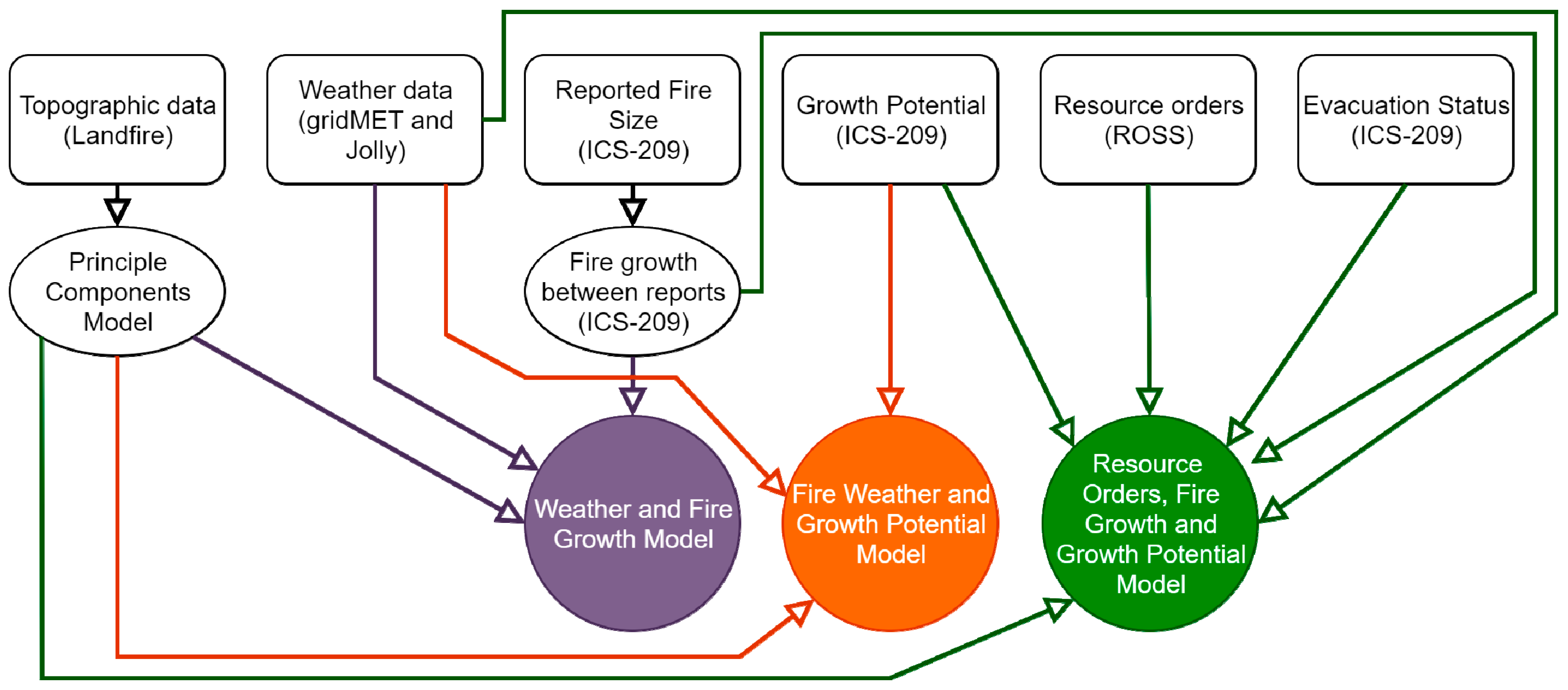
We compiled a novel dataset for this study, integrating data on fire behavior, suppression resource requests, and environmental and landscape characteristics. The data on fire behavior and operational challenges come from ICS-209 situation reports [32]. Suppression resource request data come from the Resource Ordering and Status System (ROSS) [33]. Weather data come from gridMET [34] and [35]. Vegetation data come from Landfire and the National Land Cover Database [36]. Topographic data are generated from a digital elevation model from Landfire. See

Table 2. Variable descriptions and source information of the compiled dataset.

Datasets
SIT Reports (ICS-209)	Time-varying wildfire data [32]
ROSS	Resource orders [33]
gridMET	Direct weather measurements and indices [34]
Jolly	Categorical Fire Behavior Index [35]
Landfire	Vegetation and topographic data [36]
Variable Name	Description and source
Resource	Suppression resource request counts by resource type {Type 1 Crew, Type 2 Crew, Wildland Engine, Structure Engine, Dozer, VLAT, Type 2-4 Airtanker, Helicopter} (ROSS)
Growth Potential	Subjective measure of future fire behavior {Low, Medium (baseline), High, Extreme} (ICS box 39a)
Area	Cumulative area burned (1000 acres) on day $t$
Growth	Calculated as $Are{a}_{it}-Are{a}_{it-1}$
Evacuation	Binary equal to 1 if an evacuation is ongoing
Evacuation Potential	Binary equal to 1 if there is a potential for an evacuation in the future
Inaccessibility	Subjective measure of access difficulty based on terrain {Low & Medium (baseline), High, Extreme} (ICS box 39b)
BI	Burning Index (gridMET)
ERC	Energy Release Component (gridMET)
CFBX	Categorical Fire Behavior Index (1-5) (Jolly)
Wind	Average daily windspeed in miles per hour (gridMET)
Temperature	Mean daily maximum temperature in Celsius (gridMET).
Relative Humidity	Average daily relative humidity in percent (gridMET).
Precipitation	Mean daily precipitation in millimeters (gridMET).
Day of Year	Cosine transform of day of year based on report date (ICS box 1)
Year	Categorical variable for each year (2007–2013).
GACC	Geographic Coordination Area in which ignition occurs (all excluding Southern, Eastern, and Alaska)
Cause	Categorical indicating fire cause {Human (baseline), Lightning, N/A, Under Investigation} (ICS box 8).

for a complete list of variables extracted from each data source.

The ICS-209 is the primary interagency large fire reporting (209 user guide, [37]). Different agencies have varying criteria for when an ICS-209 report is required, but, generally, these reports are submitted daily for large fires (> 100 acres in timber or > 300 acres in grass or brush), complex fires (i.e., incident management teams assigned), or fires with multi-day commitments of national resources. This form provides information on the current and anticipated fire behavior and growth potential, current fire management goals, the state of the fire’s containment, and information regarding resource use and needs (see Table 2 for variable descriptions). We use the set of ICS-209 forms to identify a set of large fires on which we could test hypotheses regarding forward- and backward-looking resource ordering patterns. We focus on large fires with long-term management plans, rather than those contained during initial attack, in order to investigate the response to change weather conditions as they evolve over the course of the fire. Thus, we built our dataset around a core set of ICS-209 single-incident fires (i.e., not multi-fire complexes) that occurred in the western US (excluding Alaska, Southern, and Eastern GACCs) from 2007–2013 with three or more reports appearing in the ICS-209 archives. We limit the data to 2013 because changes to the ICS-209 implemented in 2014 removed the question about growth potential.

We collect four variables from the ICS-209 forms: fire size, growth potential, terrain accessibility, and evacuation status. Fire size is the area burned at the time and date of the ICS-209 report. We calculate fire growth by subtracting fire size of the previous report ($t-1$) from the current report ($t$). Consequently, fire growth is an empirical measurement rather than an outcome derived from a fire spread model. Each time an ICS-209 report is filed, the IMT assesses the fire’s resistance to control along two dimensions: growth potential and terrain accessibility. Both variables take one of four values: Extreme, High, Medium, Low, or Extreme (Extreme represents the highest resistance to control). Growth potential provides us with a measurement of the IMTs perception of future fire behavior, which we hypothesize will affect the resources an IMT chooses to order. We use Inaccessibility (terrain accessibility) to control for the IMT’s perceived effectiveness of resources, which may also influence resource requests. We use “Medium” as the reference level in the growth potential and inaccessibility variables throughout our analysis.

The evacuation status on the fire is a coarse, but important, metric for assessing values at risk. The ICS-209 allows the IMT to report one or more of the following four conditions: Evacuation in progress, Potential future threat, No likely threat, and No evacuations imminent. We create a forward- and backward-looking measure of risk based on the evacuation status. The forward-looking measure is Evacuation Potential, a binary variable equal to one if there is a potential future threat of evacuation. The backward-looking variable, Evacuation, is a binary equal to one if there is an evacuation in progress.

We use resource orders submitted to the Resource Ordering and Status System (ROSS). ROSS is the primary database used to track orders and assignments of wildland fire suppression resources on large fires and intraregional resource requests (i.e., requests for resources where the resource must come from outside the home unit or a neighboring unit to respond to the incident) (https://famit.nwcg.gov/applications/ROSS). Designed for use by dispatchers, the ROSS is the most complete source of standardized information regarding resource ordering in the US (see Belval et al. [23] for data quality issues). The ICS-209 does contain information about resources committed to fires. However, we focus on resource requests rather than assignments to avoid modeling the complex dispatching decisions that determine which resources are sent to each fire (Bayham and Yoder, 2020). ROSS data includes orders from IMTs that were unable to be filled due to a scarcity of resources, which provides the most accurate information available on the preferences of the IMT. The data from ROSS includes the type of resource ordered and the date the resource is ordered. We compiled the data for each fire to obtain the total daily orders for eight categories of firefighting resources: Type 1 Crews, Type 2 Crews (which include Type 2IA Crews), Structure Engines (specified as Type 1-2 engines), Wildland Engines (specified as Type 3-7 engines), Dozers, LAT (which include Very Large and Type 1 Airtankers), Aircraft (specified as T2-4 airtankers and fixed-wing aircraft), and Helicopters (which include Type 1-3 helicopters). We merge ROSS data with incident-level data using date and common identifiers reported in the Fire Occurrence Database [38].

We use GIS to merge the fire and resource data with weather data measured or estimated near the point of fire ignition on a specific date (Figure 1). Data on the maximum daily temperature, the minimum daily humidity, the daily mean windspeed, precipitation, the Burning Index (BI), and the Energy Release Component (ERC) are extracted from gridMET, a gridded (4km resolution) daily product based on the Parameter-elevation Regressions on Independent Slopes Model (PRISM) and augmented with data from the Remote Automated Weather Station (RAWS) network weather data among others [34,39]. We also integrate the Categorical Fire Behavior Index (CFBX) [35]. The BI and ERC are commonly used indices known to influence fire behavior. CFBX is a composite index that translates BI and ERC into a discrete scale with values one through five, where one corresponds to smoldering and five corresponds to extreme erratic fire behavior.

We also used GIS to merge detailed topographic and vegetation variables constructed from the area within a 2 km radius of each fire ignition point (Figure 1). Within the buffer of each fire, we calculate the area of 20 Existing Vegetation Type (EVT) subclasses and 17 National Land Cover Database (NLCD) vegetation types. We use a digital elevation model to calculate several topographic statistics within the same 2 km buffer around each fire ignition point. Topography and vegetation are well-studied determinants of fire behavior. Our goal is to control for these factors in our regression rather than to study their effects on fire growth, which have been documented in previous research (e.g., [8,40]). Therefore, we calculate the principal components of the 104 topographic and vegetation variables (see supplement for details). We include the top 20 principal components, which represent approximately 80% of the variation in all of the topographic and vegetation variables. While the regression coefficients are difficult to interpret, principal components are ideal controls because they are orthogonal to each other by construction, which minimizes multicollinearity in regression models [41].

We begin with a core set of 18,990 observations from 2348 unique fires in the western US from 2007–2013, and we limit the dataset based on several criteria. First, we remove weather outlier observations identified as over 3 standard deviations (99.7 percentile) from the mean to mitigate their influence in the regression models. We exclude observations where the fire is reported as 100% contained to focus on the active phase of the fire, where resources would likely be ordered to control growth and protect values at risk. Additionally, we limit the dataset to observations with strictly positive growth in the analyses of fire growth and resource orders in order to focus on active phases of the fire. We compare the variation in the datasets used in each of the regressions in the supplementary material. All data processing scripts are available at https://github.com/jbayham/weather_risk_resource_orders.

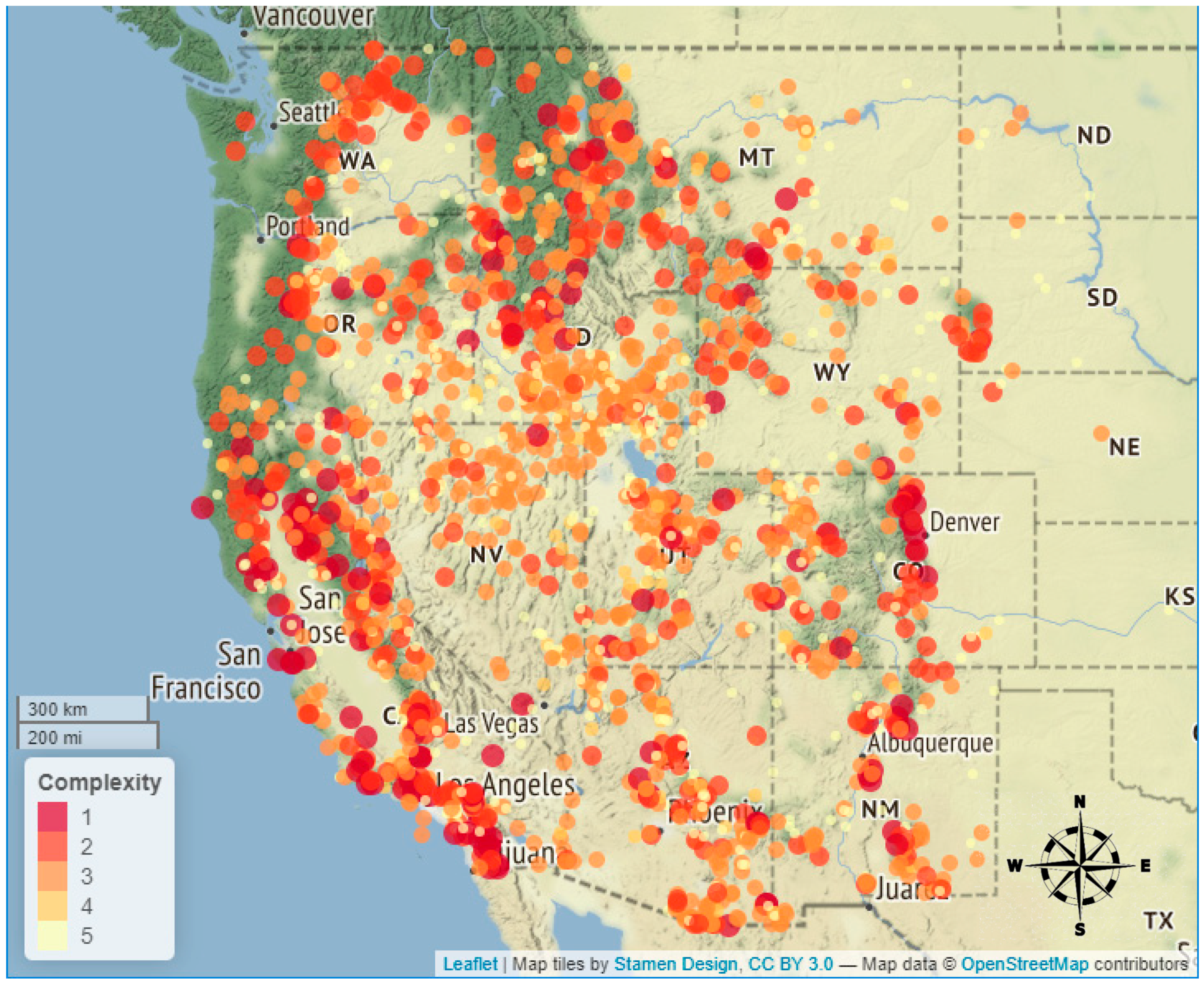
The final dataset includes 3735 complete records on 1125 fires.

Table 3. Summary Statistics of data used in all regressions.

Variable	Mean	Std. Dev.	Min	Max
Area (1000 acs.)	14.87	36.22	<1	532
Growth (1000 acs.)	1.65	2.92	<1	21
BI	58.87	13.98	26	103
ERC	71.63	13.11	25	113
Precipitation (mm)	0.40	1.37	0	13
Min Humidity (%)	16.53	8.14	1	57
Max Temperature (C)	26.86	5.88	4	45
Wind (mph)	7.92	2.80	2	18
Wildland Engines	5.19	17.49	0	318
Structure Engines	1.18	10.22	0	325
Dozers	0.65	2.83	0	65
Type 1 Crews	1.48	5.46	0	81
Type 2 Crews	0.66	1.84	0	27
LAT	0.13	0.68	0	12
Aircraft	2.23	3.88	0	31
Helicopters	0.82	1.56	0	19
Observations = 3735; Fires = 1125

includes summary statistics for the non-categorical variables in the dataset (see the supplementary material for additional information). Figure 2 displays the location of each fire in the dataset with more complex incidents indicated with larger, redder circles. The mean size of observations in the dataset is 14,870 acres, which is large because larger fires have more observations and thus receive more weight in the summary statistics. The largest fire in the data is the Wallow fire that started in AZ and burned 538,049 acres. The maximum Area is less than the 538 thousand acres because the last few thousand acres burned after the fire was considered 100% contained and thus the suppression effort can be considered over. The largest growth event was on the La Brea fire in the Los Padres NF in 2009, where the fire reportedly grew nearly 21,000 acres in an operational period. Wildland Engines are the most prevalent resource requested on a fire followed by Aircraft. While the largest maximum request was for Structure Engines (325 during the Station Fire, 2009), the mean request for Wildland Engines is larger on average (5.19).

2.3. Empirical Models

We develop a set of regression models designed to test the hypotheses outlined in Section 2.1. Our primary objective is to test whether IMTs look forward to expected fire behavior and risks or respond to realized events. We approach the objective in two steps. First, we establish an empirical relationship between weather conditions and observed fire growth. Similarly, we establish an empirical relationship between weather and a subjective assessment of future fire behavior given the information available today (growth potential). Second, we model the relationship between suppression resource orders and both growth potential and lagged fire growth, and their interactions with evacuation. Step one is intended to identify the components of weather that influence observed and expected fire growth in order to connect an IMT’s resource ordering behavior to weather conditions via fire growth. The final step investigates whether resource ordering appears to be forward- or backward-looking under differing values at risk.

2.3.1. Weather and Observed Fire Growth

We developed a model of fire growth to demonstrate the influence of weather conditions on realized fire growth. Fire growth, $growt{h}_{it}$, is the growth in the size of fire $i$ at time $t$ defined as the difference between area burned at time $t$ and area burned at time $t-1$. We specify a generalized linear regression model (quasi-Poisson) of fire growth as:

$$growt{h}_{it} = exp \left({\mathit{W}}_{it-1}^{\prime }\mathit{\beta }+f\left(A_{it-1}\right)+{\mathit{X}}_{it}^{\prime }\mathit{\varphi }+{\mathit{C}}_i^{\prime }\mathit{\gamma }\right)$$

(1)

where ${\mathit{W}}_{it-1}$ is a vector of lagged weather variables on fire $i$ at time $t$, $f\left(A_{it-1}\right)$ is a natural cubic spline of lagged fire size, ${\mathit{X}}_{it}$ is a vector of controls that vary over time, and ${\mathit{C}}_i$ is a vector if time-invariant controls. The weather vector includes the Energy Release Component (ERC), Burning Index (BI), Severe Fire Weather Potential (CFBX), precipitation, the maximum daily temperature, the minimum daily relative humidity, and the daily average wind speed. However, we estimate separate models for measured weather and composite weather variables to mitigate the effects of multicollinearity. We use lagged rather than contemporaneous weather since growth is calculated as the difference between size at time $t$ and time $t-1$.

The time-varying controls, ${\mathit{X}}_{it}$, include Inaccessibility, cosine transforms of the day of year interacted with GACC, and the burned area in the period $t-1$. The natural cubic spline of fire size captures features correlated with fire history, such as complexity. The time-invariant controls (that vary across fires) include the cause of the fire, the GACC in which the fire burned, the year, and the set of 20 topographic and vegetation principal components. We are primarily interested in the weather coefficients, $\mathit{\beta }$, which we expect to confirm the well-documented effects of weather on fire behavior.

We estimate a quasi-Poisson model because fire growth is a strictly positive variable. The quasi-Poisson model accounts for overdispersion, which makes the standard Poisson model inconsistent. Finally, we cluster standard errors at the fire level so that our results are robust to serial correlation and heteroskedasticity within a fire.

2.3.2. Weather and Growth Potential

We develop a model of growth potential to demonstrate how IMTs synthesize information about current and expected weather conditions. Growth potential, $g{p}_{it}$, is an ordered categorical variable taking values j = {Low, Medium, High, Extreme} on date $t$ of fire $i$. Therefore, we estimate the following ordered logit regression,

$$Pr \left(g{p}_{it} = j\right)=Pr \left({\kappa }_{j-1}<{\mathit{W}}_{it}^{\prime }\mathit{\delta }+f\left(A_{it-1}\right)+{\mathit{X}}_{it}^{\prime }\mathit{\theta }+{\mathit{C}}_i^{\prime }\mathit{\mu }+u_{it}<{\kappa }_j\right) \forall j$$

(2)

where ${\mathit{W}}_{it},{\mathit{X}}_{it},A_{it-1}$, and ${\mathit{C}}_i$ are defined in Equation (1), $u_{it}$ is a logistically distributed error, and ${\kappa }_j$ are a set of cut points that define the ranges corresponding to growth potential categories (Low, Medium, High, and Extreme). The goal of this model is to establish the relationship between observed weather and expected fire behavior. Again, we cluster standard errors at the fire level so that our results are robust to serial correlation and heteroskedasticity within a fire.

2.3.3. Resource Orders, Fire Growth, and Growth Potential

The last step of our analysis investigates the relationship between resource orders, realized fire growth, and expected fire growth. We specify the following fixed effects model to estimate the number of resources ordered by a fire:

$$\begin{array}{l}re{s}_{itr} = g{p}_{it}{\omega }_r+Evac{P}_{it}{\tau }_r+growt{h}_{it-1}{\eta }_r+Eva{c}_{it-1}{\psi }_r+g{p}_{it}*Evac{P}_{it}{\rho }_r+\\ growt{h}_{it-1}*Eva{c}_{it-1}{\lambda }_r+f\left(A_{it-1}\right)+{\mathit{X}}_{it}^{\prime }{\Psi }_r+ {\mathsf{\Phi }}_i+{\pi }_t+I{C}_{it}+{\epsilon }_{it}, \forall r \end{array}$$

(3)

where $g{p}_{it}$ is growth potential on fire $i$ at time $t$, $Evac{P}_{it}$ is equal to 1 if there is a potential for evacuation in the future, $growt{h}_{it-1}$ is observed fire growth in the previous period, and $Eva{c}_{it-1}$ is equal to 1 if there is an ongoing evacuation in the previous period, $f\left(A_{it-1}\right)$ is a natural cubic spline of lagged fire size, ${\mathit{X}}_{it}$ is a vector of controls that vary over time, ${\mathsf{\Phi }}_i$ are fire fixed effects (fire-specific constants), ${\pi }_t$ are time fixed effects (time-specific constants), and $I{C}_{it}$ are incident commander fixed effects. We adopt a fixed-effects strategy to estimate the impact of past fire growth and growth potential on resource orders to control for the many unobservable factors, beyond those captured by fire size, inaccessibility, and seasonal variation within GACC, all of which influence the decision to request suppression resources. These may include time and location-specific characteristics of the fire as well as social dynamics between key personnel on the incident. IMTs may change over the course of the fire, and the fixed effect captures heterogeneity in risk preferences and management style [21].

We include interactions of growth potential and evacuation potential as well as growth and ongoing evacuations as measures of risk. We expect IMTs to respond differently to expected or observed fire growth if there are values at risk. However, it is not clear a priori how exactly IMTs should respond when the fire is resistant to control, and there are values at risk. On the one hand, more resources may facilitate safe evacuation and protect life. On the other hand, engaging the fire with more resources may put firefighters’ lives at risk.

We use lags of evacuation and fire growth to remove the potential for reverse causality. In principle, lagged evacuation and fire growth are determined at time $t$ when requests are made. We cluster standard errors at the fire level so that our results are robust to serial correlation and heteroskedasticity within a fire. The regressions are estimated in R and Stata statistical software [42,43]. The fixed effect regressions are estimated using the fixest package in R [44].

3. Results

The results section will follow the two-step structure outlined in Section 2.3. First, we present the results demonstrating the relationship between weather and observed fire growth and subjective growth potential. Second, we present results connecting the observed fire growth and subjective growth potential to suppression resource requests. Our results illustrate the pathway through which realizations and expectations of uncertain weather impact suppression resource requests.

3.1. Weather, Fire Growth, and Growth Potential

The results of the quasi-Poisson regression suggest that weather conditions have a statistically significant effect on observed fire growth. We estimated three models: (1) with direct weather measurements (temperature, humidity, precipitation, and humidity), (2) with ERC and BI, and (3) with CFBX. We estimate separate models of fire growth because the composite weather indices are highly collinear with the direct weather measurements. We estimate the regressions with an expanded dataset since there were more complete observations of the variables used in Equation (1). We compare the summary statistics of the expanded dataset with those in Table 3 in the supplementary material to show that the additional observations improve the precision of the estimates. Standard errors are clustered at the fire level and are robust to heteroscedasticity and serial correlation within a fire. Full regression tables are available in Supplementary Table S2.

Figure 3 displays the marginal effects of select weather conditions on fire growth. For reference, the mean fire growth is 1.65 (1000 acres). The results generally confirm the intuition that high temperature, ERC, and CFBX increase fire growth while high humidity reduces fire growth. The figures indicate that these effects are nonlinear with significantly larger fire growth occurring at the upper quartile of ERC and temperature levels. The highest CFBX category, which is described as extreme and erratic fire behavior, is correlated with higher levels of growth, while the lower two categories described as smoldering, creeping, and spreading correspond to much lower levels of fire growth.

Next, we investigated the relationship between weather conditions and expected fire behavior using an ordered logit model. Again, we estimate two separate models for direct weather measurement and composite indices. We cluster standard errors at the fire level to account for heteroscedasticity and serial correlation within a fire. Full regression tables are available in Supplementary Table S3.

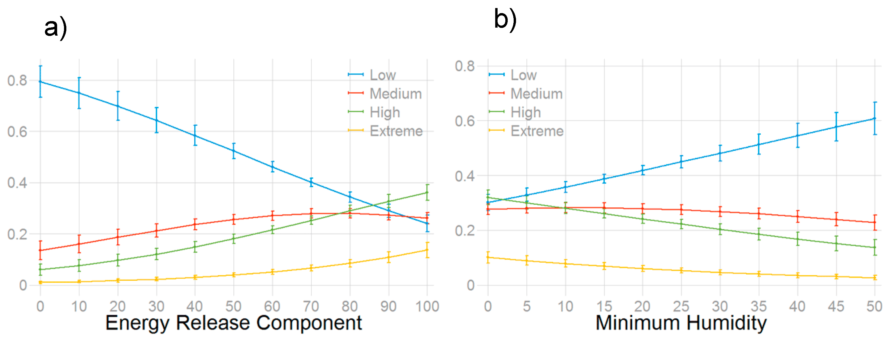
Figure 4 illustrates the predicted probabilities of growth potential categories as a function of the ERC and Minimum Humidity. Panel (a) suggests that low growth potential is highly likely (probability of 0.80) at low ERC levels. As ERC increases, IMTs become increasingly likely to report medium, high, and extreme growth potential. When the ERC is 100, IMTs are most likely to report high growth potential. In contrast, when humidity is low, IMTs are most likely to report high growth potential (green line in panel (b)). As humidity rises, IMTs become increasingly likely to report low growth potential. These results suggest that IMTs develop expectations about fire behavior based on current and expected weather conditions. While we do not use data on forecasted weather, we have estimated the model with forward lags of realized weather and find that the results are qualitatively similar.

3.2. Suppression Resources, Fire Growth, and Growth Potential

The second step of our analysis investigates the relationship between observed fire growth and growth potential on resource orders. First, we estimate a model of total resource requests under four specifications to illustrate the interaction between weather-driven fire behavior and values at risk. We then estimate separate regressions for each type of resource to investigate whether resource types respond to weather differently based on their intended functions. Full regression tables are available in Supplementary Tables S4 and S5.

Table 4. Linear fixed effects regression of total resource requests.

	(1)	(2)	(3)	(4)
Growth Potential (High)	10.5795 *** (2.2232)	10.2399 *** (2.5257)	7.2662 *** (2.3789)	7.6294 ** (3.6203)
Growth Potential (Low)	−6.601 ** (2.9824)	−5.5504 ** (2.3694)	−1.9734 (2.1306)	1.7124 (3.2106)
Lagged Growth	0.593 (0.4038)	0.3376 * (0.1903)	0.4589 ** (0.2102)	0.4447 (0.2921)
Potential Evacuation		−0.1334 (3.3062)	−1.3574 (3.2013)	−1.0775 (4.3369)
Lagged Evacuation		−1.1129 (3.594)	−1.5337 (3.8048)	−3.2708 (4.9227)
Growth Potential (High) × Pot. Evac.		0.488 (3.8585)	2.1315 (3.7043)	−0.7307 (4.9029)
Growth Potential (Low) × Pot. Evac.		−8.6827 (12.6131)	−12.1008 (12.3487)	−14.3315 (18.1677)
Lagged Growth × L. Evacuation		0.4107 (0.6001)	0.3392 (0.6056)	0.3819 (0.9442)
Fixed−Effects:
Fire	Yes	Yes	Yes	Yes
Days Since Discovery	No	No	Yes	Yes
Incident Commander	No	No	No	Yes
R2	0.580	0.581	0.623	0.765
Within R2	0.126	0.128	0.054	0.048

* p < 0.1; ** p < 0.05; *** p < 0.01; Observations: 3735; Fires: 1125; Number of days since discovery FE: 84; Number of ICs: 1234; Medium Growth Potential is the omitted category. Interactions between variables are denoted with an x. Omitted controls include: Inaccessibility, the day of the year * GACC, and a natural cubic spline of fire size.

shows the results of four regressions, all with total resource requests as the dependent variable. Standard errors are clustered at the fire and are robust to heteroscedasticity and serial correlation within a fire in all specifications. Column 1 displays the results of the regression with only growth potential and lagged growth with fire fixed effects. The results indicate that high growth potential (high and extreme categories) leads to 10.58 more total resource requests relative to a growth potential of medium. Similarly, low growth potential leads to 6.6 fewer requests relative to medium growth potential. While the coefficient on lagged growth is positive, it is imprecisely estimated and indistinguishable from 0 at an alpha = 0.05.

Column 2 shows the results of a similar model, but we have added potential evacuation and lagged evacuation (ongoing evacuation reported in period $t-1$) as well as their interactions with growth potential and lagged growth, respectively. Growth potential remains a statistically significant driver of resource requests. Lagged growth is now also statistically significant, indicating that an additional 1000 acres of fire growth in the previous operational period increase resource requests by 0.34 resources. While the coefficients on the interaction terms are not statistically significant, the signs indicate that an ongoing or potential evacuation exacerbates the response. Together, these results provide support for our hypotheses that managers are forward- and backward-looking with regard to perimeter control objectives (Table 1). Moreover, the stability of the growth potential coefficient estimates in Columns (1) and (2) suggest that while potential evacuation and growth potential may be correlated, it is not severe enough to substantially affect the growth potential coefficient estimates.

Columns 3 and 4 include the same regressors as Column 2, with additional fixed effects for the time since fire discovery and the incident commander. These alternative specifications are intended to assess the robustness of our estimates to additional control variables. The coefficient on high growth potential remains statistically significant across all models, indicating a robust influence on resource ordering. The coefficients on the other covariates do not remain statistically significant, casting doubt on the robustness of the influence of lagged growth and interactions with evacuation status on resource ordering.

The intention of our model is to estimate the causal impact of observed and expected growth as well as evacuation on resource orders. While the coefficient estimates do not depend on model fit, we present the overall and within R2 estimates. The overall R2 increases as more variables (or fixed effects) are added to the model. The estimates range from 0.58 in Column 1 to 0.76 in Column 4, indicating that our model explains between 58% and 76% of the variation in the total resources ordered. The within R2 estimates provide information about the explanatory power of regressors net of the fixed effects. The within R2 of Model 2 indicates that the parsimonious specification with only fire fixed effects performs better than the models with time since discovery and IC fixed effects. These results indicate that resource orders are difficult to model because they depend on the inherent complexity of fire management.

We now estimate the specification in Column 2, Table 4, for each resource type individually to investigate heterogeneity in the forward- and backward-looking ordering patterns.

Table 5. Linear fixed effect regression of select suppression resources.

	Wildland Engines	Structure Engines	Type 1 Crews	Type 2 Crews
Growth Potential (High)	4.7291 *** (1.2993)	0.6385 (0.6829)	1.4889 *** (0.4261)	0.216 (0.1377)
Growth Potential (Low)	−1.6283 (1.1496)	−1.2824 * (0.7419)	−0.5578 (0.4137)	−0.1922 ** (0.0973)
Lagged Growth	0.3424 (1.7795)	0.215 (0.8521)	−0.2072 (0.6257)	−0.2593 (0.1712)
Potential Evacuation	0.1789 * (0.1012)	−0.0128 (0.0529)	0.039 (0.0305)	0.0266 ** (0.0133)
Lagged Evacuation	−0.9957 (2.1646)	0.2496 (1.152)	−0.4623 (0.6051)	0.2156 (0.2102)
Growth Potential (High) × Pot. Evac.	0.0566 (2.1386)	−0.3236 (1.0192)	0.3658 (0.6758)	0.5029 ** (0.2375)
Growth Potential (Low) × Pot. Evac.	−4.2669 (6.0111)	−3.7647 (4.7297)	−0.6825 (1.4989)	0.5224 (0.399)
Lagged Growth × L. Evacuation	0.1994 (0.3822)	0.0112 (0.0937)	0.135 (0.1182)	−0.0068 (0.0252)
Fixed-Effects:
Fire	Yes	Yes	Yes	Yes
R2	0.49577	0.46379	0.5019	0.3285
Within R2	0.08948	0.02522	0.08185	0.05616

* p < 0.1; ** p < 0.05; *** p < 0.01; Observations: 3735; Fires: 1125; Number of days since discovery FE: 84; Number of IMTs: 1234; Medium Growth Potential is the omitted category. Interactions between variables are denoted with an x. Omitted controls include: Inaccessibility, the day of the year * GACC, and a natural cubic spline of fire size.

and

Table 6. Linear fixed effect regression of select suppression resources.

	LAT	Aircraft	Helicopters	Dozers
Growth Potential (High)	0.1248 *** (0.0392)	1.9236 *** (0.3373)	0.5449 *** (0.1322)	0.5739 ** (0.2379)
Growth Potential (Low)	−0.1286 ** (0.0596)	−1.2483 *** (0.3465)	−0.2537 ** (0.1256)	−0.259 (0.1977)
Lagged Growth	0.0123 (0.0566)	−0.0139 (0.4454)	−0.0819 (0.1736)	−0.1409 (0.2494)
Potential Evacuation	−0.0011 (0.003)	0.0669 ** (0.0336)	0.0259 ** (0.0119)	0.0142 (0.0171)
Lagged Evacuation	−0.0133 (0.0487)	0.4844 (0.3392)	−0.1368 (0.1582)	−0.4544 (0.3481)
Growth Potential (High) × Pot. Evac.	0.0001(0.0687)	−0.1609 (0.4953)	−0.0279 (0.207)	0.0748 (0.291)
Growth Potential (Low) × Pot. Evac.	0.0231 (0.1141)	0.3449 (0.8261)	0.1262 (0.3358)	−0.9853 (0.9743)
Lagged Growth × L. Evacuation	0.01 (0.0069)	0.0147 (0.0398)	0.0111 (0.0162)	0.036 (0.0535)
Fixed-Effects:
Fire	Yes	Yes	Yes	Yes
R2	0.62267	0.63442	0.48125	0.44901
Within R2	0.02399	0.17992	0.12463	0.07102

* p < 0.1; ** p < 0.05; *** p < 0.01; Observations: 3735; Fires: 1125; Number of days since discovery FE: 84; Number of ICs: 1234; Medium Growth Potential is the omitted category. Interactions between variables are denoted with an x. Omitted controls include: Inaccessibility, the day of the year * GACC, and a natural cubic spline of fire size.

show the results of the individual resource regressions. High growth potential leads IMTs to request more Wildland Engines, Type 1 Crews, Dozers, LAT, Aircraft, and Helicopters (High growth potential estimates not statistically significant for Structure Engines and Type 2 Crews). The magnitude of the estimates indicates that nearly twice as many resources are requested when growth potential is high relative to the medium growth potential. For example, the coefficient estimate on Wildland Engines is 4.73 (Table 5), whereas the unconditional mean in the sample is 5.19 (Table 3). Similarly, we find robust evidence that low growth potential leads IMTs to request fewer resources relative to the medium growth potential (not statistically significant for Wildland Engines, Type 1 Crews, and Dozers). However, the magnitude of the low growth potential coefficients is smaller than the high growth potential counterpart in most cases, indicating that the effect is asymmetric, with more weight placed on high growth potential.

The coefficient estimates on the other variables are not consistent across resource types. There is some limited evidence that IMTs order more resources in response to a Potential Evacuation, but the magnitudes are relatively small. The estimates are statistically significant for Wildland Engines, Type 2 Crews, Aircraft, and Helicopters. Moreover, only the coefficient on the interaction between high Growth Potential and Potential Evacuation is statistically significant in the Type 2 Crew model. These results provide limited evidence that IMTs respond to our constructed measure of risk.

4. Discussion

We find robust evidence supporting the view that weather conditions influence observed and expected fire behavior and that IMTs are generally forward-looking when ordering resources. Direct measures of the weather and weather indices have statistically significant impacts on fire growth, a finding that is consistent with prior literature—warmer, dryer, and windier conditions increase growth, while cooler, wetter, and calmers conditions mitigate growth [5,39]. Our model of growth potential indicates that IMTs internalize current and forecasted weather to form expectations about future fire activity. Our model of resource orders shows that IMTs respond predominantly to expectations about future fire activity rather than recently observed growth events. Together these results suggest that IMTs appear to be more forward-looking rather than backward-looking.

While our regression models are estimated separately, we can combine the results to draw inferences about how weather influences resource ordering. The first step in our modeling process establishes the relationship between measured weather or weather index and observed growth and growth potential. The results in Figure 4a show how the ERC relates to the probability that IMTs report different growth potential categories. For example, at ERC = 0, the probability of an IMT reporting high growth potential (green line) is approximately 0.10 (10%) and increases nonlinearly until the probability is nearly 0.40 at ERC = 100. The growth potential probabilities can be mapped through the regression results in Table 4 to estimate how the ERC will ultimately impact resource orders. The predicted number of resources ordered on a fire with medium growth potential (assuming mean values for all other regressors) is 3.87. As the ERC increases, the probability of high growth potential increases, which can be multiplied by the high growth potential coefficient in Table 4 (10.24). Using the example from above, the probability of high growth potential is 0.40 at ERC = 100, which increases total resource orders by 4.96 (0.40*10.24). We also need to account for the probability of low growth, which decreases orders by 1.22 (0.22*(−5.55)). The net increase in resource orders at ERC = 100 is 3.74 (4.96–1.22).

We find little evidence to support our hypotheses regarding structure protection objectives and our constructed metric for risk, which is defined as the interaction between observed or potential evacuation and observed or expected growth. We expected to find that resources adept at structure protection would be requested more often in the event that an evacuation was necessary. However, we only found evidence of more requests for Wildland Engines, Type 2 Crews, Aircraft, and Helicopters when there is a potential for evacuation. The combined risk (growth potential and potential evacuation interaction) is significant in the Type 2 Crew model only. These results may simply reflect the large variation in an IMT’s use and perception of resource availability and abilities [21,45]. In addition, our risk metric may be an incomplete measure of the full set of values at risk, which may influence resource ordering patterns. The metric may be conflating the need for structure protection with the role of coordination and the use of different resources as emergency responders [46]. Future research may focus on developing a more precise quantitative measure of risk factors that influence resource requests.

The R² estimates in Table 4, Table 5 and Table 6 suggest that the models only explain up to 70% of the variation in total resource orders, which implies that 30% or more variation is unexplained. This result is consistent with Simpson et al. [47] who find that resources are used in various ways throughout the suppression effort. While we limit the dataset to focus on the phase of active suppression, it is likely that a complex array of factors beyond those captured in our regression model influences ordering patterns [48,49].

Fire growth and values at risk are not independent. Valued assets are at risk of damage if the fire is expected to grow to such an extent that the asset is exposed to fire. This dependence of values at risk on fire growth makes it difficult to statistically distinguish between the effect of fire growth and the values at risk. We attempt to parse out these effects by treating evacuation as a modifier on observed or expected fire growth. However, our results do not provide strong evidence that values at risk (as measured by evacuation) dramatically change the importance of responding to expected fire growth. Future analyses may consider a spatiotemporal measure of values at risk, such as homes within some buffer of the daily fire perimeter.

Our analysis captures a likely pathway through which incident management teams translate weather-driven expectations about fire behavior into resource orders. However, the variable growth potential is limited to four categories, which may mask variation in response to certain condition combinations. For instance, high winds may promote fire growth, but they may also limit the ability to use aircraft resources. An IMT may request fewer aircraft resources during high wind events. On the other hand, IMTs may request an aircraft so that they are prepared once the wind subsides. Our consistently significant estimates on growth potential suggest that the IMTs request more resources regardless of the factors driving higher fire activity.

While our results suggest that IMTs order resources based on expected fire growth, we do not know how the resources are used or whether they were effective in achieving their objective. While simulation models provide a framework through which one is able to analyze cost-efficient and effective responses, crucial model parameters are collected from lab experiments, which may or may not reflect actual conditions faced during a suppression effort. Analysts need highly resolved spatiotemporal data on fire behavior and suppression activity in order to estimate effectiveness parameters. Current legislative mandates may standardize the use of tracking equipment, which may provide this information on future fires. These data have the potential to mitigate firefighter safety risks and develop a better understanding of the drivers of resource use over the course of the fire. The results of our analysis complement efforts to quantify suppression effectiveness by characterizing the linkage between variable weather conditions and resource ordering patterns.

5. Conclusions

We develop a two-step regression framework to estimate the pathways through which weather effects resource ordering patterns. We find robust evidence that incident commanders are forward-looking and order resources in response to expected weather-driven fire growth events as opposed to simply reacting to the observed conditions and fire behavior. Incident commanders order nearly twice as many resources when they expect high fire growth potential. These results suggest that incident commanders may be trying to manage weather risk in a highly complex environment.

The results of this analysis have practical applications and policy implications. Our analysis highlights the significant role that variable weather plays in resource ordering behavior. Our results could be coupled with weather forecasts to estimate demands on the stock of wildfire suppression resources. Moreover, fire size, damage, and complexity are expected to increase under future climate scenarios, placing additional strain on suppression resources [39,50]. Beyond the trends of rising temperatures and drying fuels, short-term weather events are expected to drive erratic and challenging fire conditions. Our analysis provides a framework through which one is able to understand how future weather variability may impact resource demands

References

- Tedim, F.; Leone, V.; Amraoui, M.; Bouillon, C.; Coughlan, M.R.; Delogu, G.M.; Fernandes, P.M.; Ferreira, C.; McCaffrey, S.; McGee, T.K.; et al. Defining Extreme Wildfire Events: Difficulties, Challenges, and Impacts. Fire 2018, 1, 9. [Google Scholar] [CrossRef] [Green Version]
- Coen, J.L.; Cameron, M.; Michalakes, J.; Patton, E.G.; Riggan, P.J.; Yedinak, K.M. WRF-Fire: Coupled Weather–Wildland Fire Modeling with the Weather Research and Forecasting Model. J. Appl. Meteor. Clim. 2012, 52, 16–38. [Google Scholar] [CrossRef]
- Jolly, W.M.; Cochrane, M.A.; Freeborn, P.H.; Holden, Z.A.; Brown, T.J.; Williamson, G.J.; Bowman, D.M.J.S. Climate-induced variations in global wildfire danger from 1979 to 2013. Nat. Commun. 2015, 6, 1–11. [Google Scholar] [CrossRef] [PubMed]
- Bessie, W.C.; Johnson, E.A. The Relative Importance of Fuels and Weather on Fire Behavior in Subalpine Forests. Ecology 1995, 76, 747–762. [Google Scholar] [CrossRef] [Green Version]
- Collins, B.M. Fire weather and large fire potential in the northern Sierra Nevada. Agric. Meteorol. 2014, 189–190, 30–35. [Google Scholar] [CrossRef]
- Holmes, T.P.; Calkin, D.E. Econometric analysis of fire suppression production functions for large wildland fires. Int. J. Wildland Fire 2013, 22, 246–255. [Google Scholar] [CrossRef] [Green Version]
- Katuwal, H.; Calkin, D.E.; Hand, M.S. Production and efficiency of large wildland fire suppression effort: A stochastic frontier analysis. J. Env. Manag. 2016, 166, 227–236. [Google Scholar] [CrossRef]
- Hand, M.S.; Thompson, M.P.; Calkin, D.E. Examining heterogeneity and wildfire management expenditures using spatially and temporally descriptive data. J. For. Econ. 2016, 22, 80–102. [Google Scholar] [CrossRef] [Green Version]
- Belval, E.J.; O’Connor, C.D.; Thompson, M.P.; Hand, M.S. The Role of Previous Fires in the Management and Expenditures of Subsequent Large Wildfires. Fire 2019, 2, 57. [Google Scholar] [CrossRef] [Green Version]
- Masarie, A.T.; Wei, Y.; Belval, E.J.; Thompson, M.P.; Oprea, I.; Tabatabaei, M.; Calkin, D.E. Valuating fire suppression risk data. Appl. Math. Model. 2019, 69, 93–112. [Google Scholar] [CrossRef]
- Belval, E.J.; Wei, Y.; Calkin, D.E.; Stonesifer, C.S.; Thompson, M.P.; Tipton, J.R. Studying interregional wildland fire engine assignments for large fire suppression. Int. J. Wildland Fire 2017, 26, 642–653. [Google Scholar] [CrossRef]
- Belval, E.J.; Calkin, D.E.; Wei, Y.; Stonesifer, C.S.; Thompson, M.P.; Masarie, A. Examining dispatching practices for Interagency Hotshot Crews to reduce seasonal travel distance and manage fatigue. Int. J. Wildland Fire 2018, 27, 569–580. [Google Scholar] [CrossRef] [Green Version]
- Bayham, J.; Yoder, J. Resource Allocation Under Fire. Land Econ. 2020, 96, 92–110. [Google Scholar] [CrossRef] [Green Version]
- Calkin, D.E.; Venn, T.; Wibbenmeyer, M.; Thompson, M.P. Estimating US federal wildland fire managers’ preferences toward competing strategic suppression objectives. Int. J. Wildland Fire 2013, 22, 212. [Google Scholar] [CrossRef]
- Wibbenmeyer, M.J.; Hand, M.S.; Calkin, D.E.; Venn, T.J.; Thompson, M.P. Risk Preferences in Strategic Wildfire Decision Making: A Choice Experiment with U.S. Wildfire Managers. Risk Anal. 2013, 33, 1021–1037. [Google Scholar] [CrossRef]
- Hand, M.S.; Wibbenmeyer, M.J.; Calkin, D.E.; Thompson, M.P. Risk Preferences, Probability Weighting, and Strategy Tradeoffs in Wildfire Management. Risk Anal. 2015, 35, 1876–1891. [Google Scholar] [CrossRef]
- Thompson, M.P.; Calkin, D.E.; Herynk, J.; McHugh, C.W.; Short, K.C. Airtankers and wildfire management in the US Forest Service: Examining data availability and exploring usage and cost trends. Int. J. Wildland Fire 2013, 22, 223–233. [Google Scholar] [CrossRef]
- Calkin, D.E.; Stonesifer, C.S.; Thompson, M.P.; McHugh, C.W. Large airtanker use and outcomes in suppressing wildland fires in the United States. Int. J. Wildland Fire 2014, 23, 259. [Google Scholar] [CrossRef]
- Stonesifer, C.S.; Calkin, D.E.; Thompson, M.P.; Stockmann, K.D. Fighting fire in the heat of the day: An analysis of operational and environmental conditions of use for large airtankers in United States fire suppression. Int. J. Wildland Fire 2016, 25, 520–533. [Google Scholar] [CrossRef]
- Thompson, M.; Lauer, C.; Calkin, D.; Rieck, J.; Stonesifer, C.; Hand, M. Wildfire Response Performance Measurement: Current and Future Directions. Fire 2018, 1, 21. [Google Scholar] [CrossRef] [Green Version]
- Hand, M.; Katuwal, H.; Calkin, D.E.; Thompson, M.P. The influence of incident management teams on the deployment of wildfire suppression resources. Int. J. Wildland Fire 2017, 26, 615. [Google Scholar] [CrossRef]
- Katuwal, H.; Dunn, C.J.; Calkin, D.E. Characterising resource use and potential inefficiencies during large-fire suppression in the western US. Int. J. Wildland Fire 2017, 26, 604. [Google Scholar] [CrossRef]
- Belval, E.J.; Stonesifer, C.S.; Calkin, D.E. Fire suppression resource scarcity: Current metrics and future performance indicators. 2020; In Review. [Google Scholar]
- Calkin, D.E.; Gebert, K.M.; Jones, J.G.; Neilson, R.P. Forest Service Large Fire Area Burned and Suppression Expenditure Trends, 1970–2002. J. For. 2005, 103, 179–183. [Google Scholar] [CrossRef]
- Short, K.C. Sources and implications of bias and uncertainty in a century of US wildfire activity data. Int. J. Wildland Fire 2015, 24, 883. [Google Scholar] [CrossRef]
- Wei, Y.; Belval, E.J.; Thompson, M.P.; Calkin, D.E.; Stonesifer, C.S. A simulation and optimisation procedure to model daily suppression resource transfers during a fire season in Colorado. Int. J. Wildland Fire. 2016, 26, 630–641. [Google Scholar] [CrossRef] [Green Version]
- Haight, R.G.; Fried, J.S. Deploying Wildland Fire Suppression Resources with a Scenario-Based Standard Response Model. INFOR 2007, 45, 31–39. [Google Scholar] [CrossRef]
- Wei, Y.; Thompson, M.P.; Haas, J.R.; Dillon, G.K.; O’Connor, C.D. Spatial optimization of operationally relevant large fire confine and point protection strategies: Model development and test cases. Can. J. Res. 2018, 48, 480–493. [Google Scholar] [CrossRef] [Green Version]
- Dunn, C.J.; Thompson, M.P.; Calkin, D.E. A framework for developing safe and effective large-fire response in a new fire management paradigm. For. Ecol. Manag. 2017, 404, 184–196. [Google Scholar] [CrossRef]
- Petrovic, N.; Carlson, J.M. A decision-making framework for wildfire suppression. Int. J. Wildland Fire 2012, 21, 927–937. [Google Scholar] [CrossRef]
- Kolden, C.A.; Henson, C. A Socio-Ecological Approach to Mitigating Wildfire Vulnerability in the Wildland Urban Interface: A Case Study from the 2017 Thomas Fire. Fire 2019, 2, 9. [Google Scholar] [CrossRef] [Green Version]
- FAMWEB. SIT-209; U.S. Department of Agriculture Forest Service Fire and Aviation Management. Available online: https://fam.nwcg.gov/fam-web/ (accessed on 1 January 2020).
- Lockheed Martin Enterprise Solutions & Services. Resource Ordering and Status System (ROSS). 2012. Available online: https://famit.nwcg.gov/applications/ROSS (accessed on 31 December 2019).
- Abatzoglou, J.T. Development of gridded surface meteorological data for ecological applications and modelling. Int. J. Clim. 2013, 33, 121–131. [Google Scholar] [CrossRef]
- Jolly, W.M.; Freeborn, P.H. Towards improving wildland firefighter situational awareness through daily fire behaviour risk assessments in the US Northern Rockies and Northern Great Basin. Int. J. Wildland Fire 2017, 26, 574–586. [Google Scholar] [CrossRef]
- LANDFIRE. LANDFIRE (2013, January-last Update); U.S. Department of Agriculture, Forest Service and U.S. Department of Interior: Washington, DC, USA, 2013.
- NIFC. 209 Program User’s Guide (2011); National Interagency Fire Center: Boise, ID, USA, 2011. [Google Scholar]
- Short, K.C. Spatial Wildfire Occurrence Data for the United States, 1992–2015 (FPA_FOD_20170508), 4th ed.; Forest Service Research Data Archive: Fort Collins, CO, USA, 2017. [Google Scholar] [CrossRef]
- Abatzoglou, J.T.; Williams, A.P. Impact of anthropogenic climate change on wildfire across western US forests. PNAS 2016, 113, 11770–11775. [Google Scholar] [CrossRef] [PubMed] [Green Version]
- Gebert, K.M.; Calkin, D.E.; Yoder, J. Estimating Suppression Expenditures for Individual Large Wildland Fires. West J. Appl. For. 2007, 22, 188–196. [Google Scholar] [CrossRef] [Green Version]
- Greene, W.H. Econometric Analysis; Prentice Hall: Boston, MA, USA, 2012; ISBN 0-13-139538-6. [Google Scholar]
- StataCorp. Stata Statistical Software; StataCorp LP: College Station, TX, USA, 2015. [Google Scholar]
- R Core Team. R: A Language and Environment for Statistical Computing; R Foundation for Statistical Computing: Vienna, Austria, 2019. [Google Scholar]
- Berge, L. Efficient Estimation of Maximum Likelihood Models with Multiple Fixed-Effects: The R Package FENmlm. Available online: https://EconPapers.repec.org/RePEc:luc:wpaper:18-13 (accessed on 31 December 2019).
- Stonesifer, C.S.; Calkin, D.E.; Hand, M.S. Federal fire managers’ perceptions of the importance, scarcity and substitutability of suppression resources. Int. J. Wildland Fire 2017, 26, 598. [Google Scholar] [CrossRef]
- Steelman, T.; Nowell, B. Evidence of effectiveness in the Cohesive Strategy: Measuring and improving wildfire response. Int. J. Wildland Fire 2019, 28, 267–274. [Google Scholar] [CrossRef]
- Simpson, H.; Bradstock, R.; Price, O. A Temporal Framework of Large Wildfire Suppression in Practice, a Qualitative Descriptive Study. Forests 2019, 10, 884. [Google Scholar] [CrossRef] [Green Version]
- Donovan, G.H.; Prestemon, J.P.; Gebert, K. The Effect of Newspaper Coverage and Political Pressure on Wildfire Suppression Costs. Soc. Nat. Resour. 2011, 24, 785–798. [Google Scholar] [CrossRef] [Green Version]
- Canton-Thompson, J.; Gebert, K.M.; Thompson, B.; Jones, G.; Calkin, D.; Donovan, G. External Human Factors in Incident Management Team Decisionmaking. J. For. 2008, 106, 416–424. [Google Scholar]
- Hope, E.S.; McKenney, D.W.; Pedlar, J.H.; Stocks, B.J.; Gauthier, S. Wildfire Suppression Costs for Canada under a Changing Climate. PLoS ONE 2016, 11, e0157425. [Google Scholar] [CrossRef] [Green Version]
Figure 1.
Data processing diagram to illustrate how key variables and data sources are integrated to produce the dataset used for analysis.
Figure 2.
Map of fires in the dataset. The most complex incidents are represented with the largest and darkest dots. Incident complexity is not a variable used in the model but is a composite measure incorporating fire size and values at risk. An interactive version of the map is in the Supplementary Materials.
Figure 3.
Predicted fire growth response to relevant weather conditions: (a) Energy Release Component, (b) Categorical Fire Behavior Index, (c) Relative Humidity, and (d) Maximum Temperature. The black lines represent the predicted fire growth, and the shaded area represents 95% confidence intervals from the quasi-Poisson regression of fire growth on weather conditions. The red dashed lines are the mean growth in the data (1.65 from Table 3). The small hash marks along the horizontal axis indicate the density of observations.
Figure 4.
Predicted Probabilities of Growth Potential as a function of (a) the Energy Release Component and (b) Relative Humidity (%). The lines represent point estimates, while the bars represent 95% confidence intervals.