Using Count Data Models to Predict Epiphytic Bryophyte Recruitment in Schima superba Gardn. et Champ. Plantations in Urban Forests

 , ,
, , 
Abstract
:1. Introduction
2. Materials and Methods
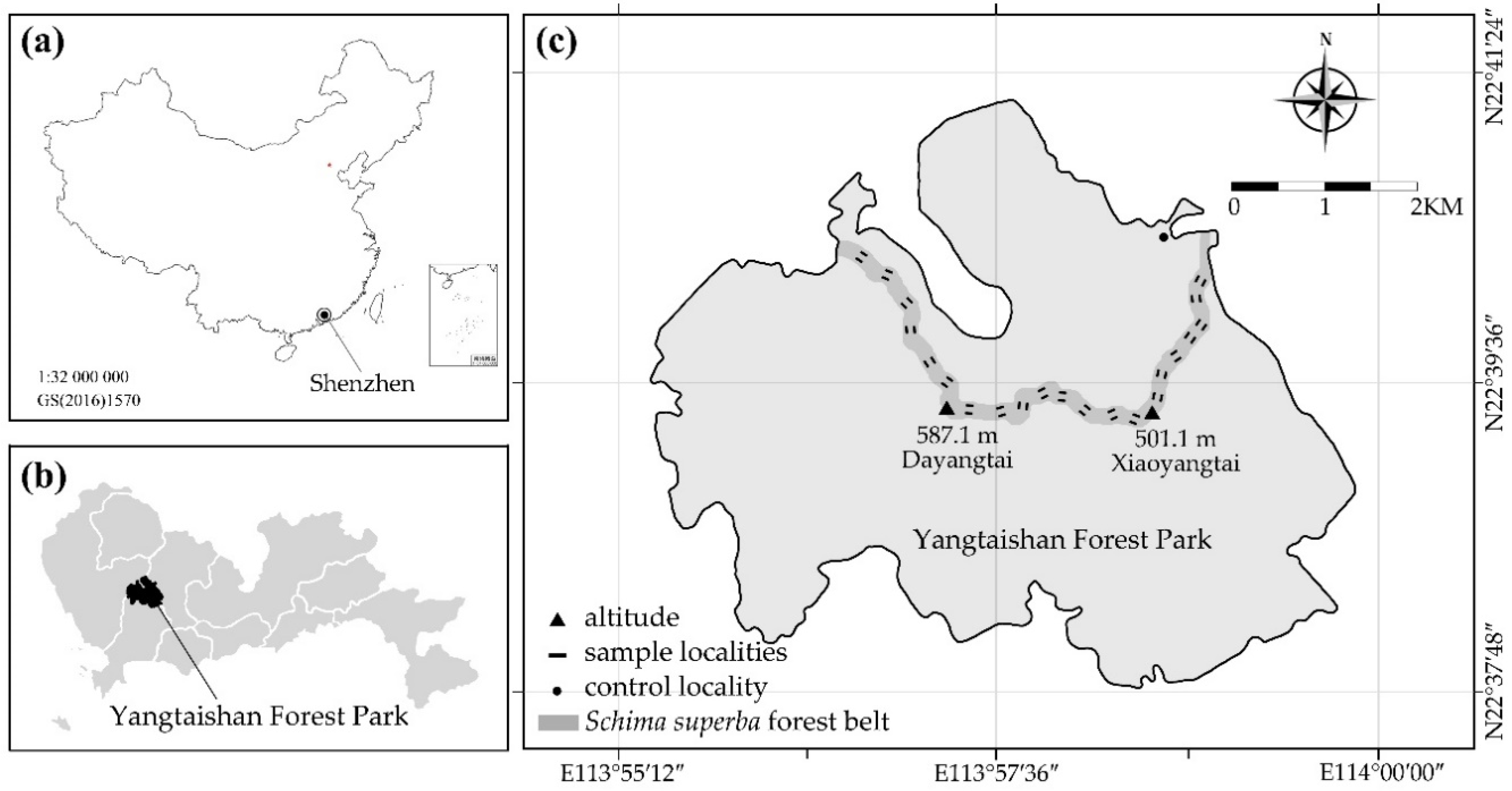
2.1. Study Area
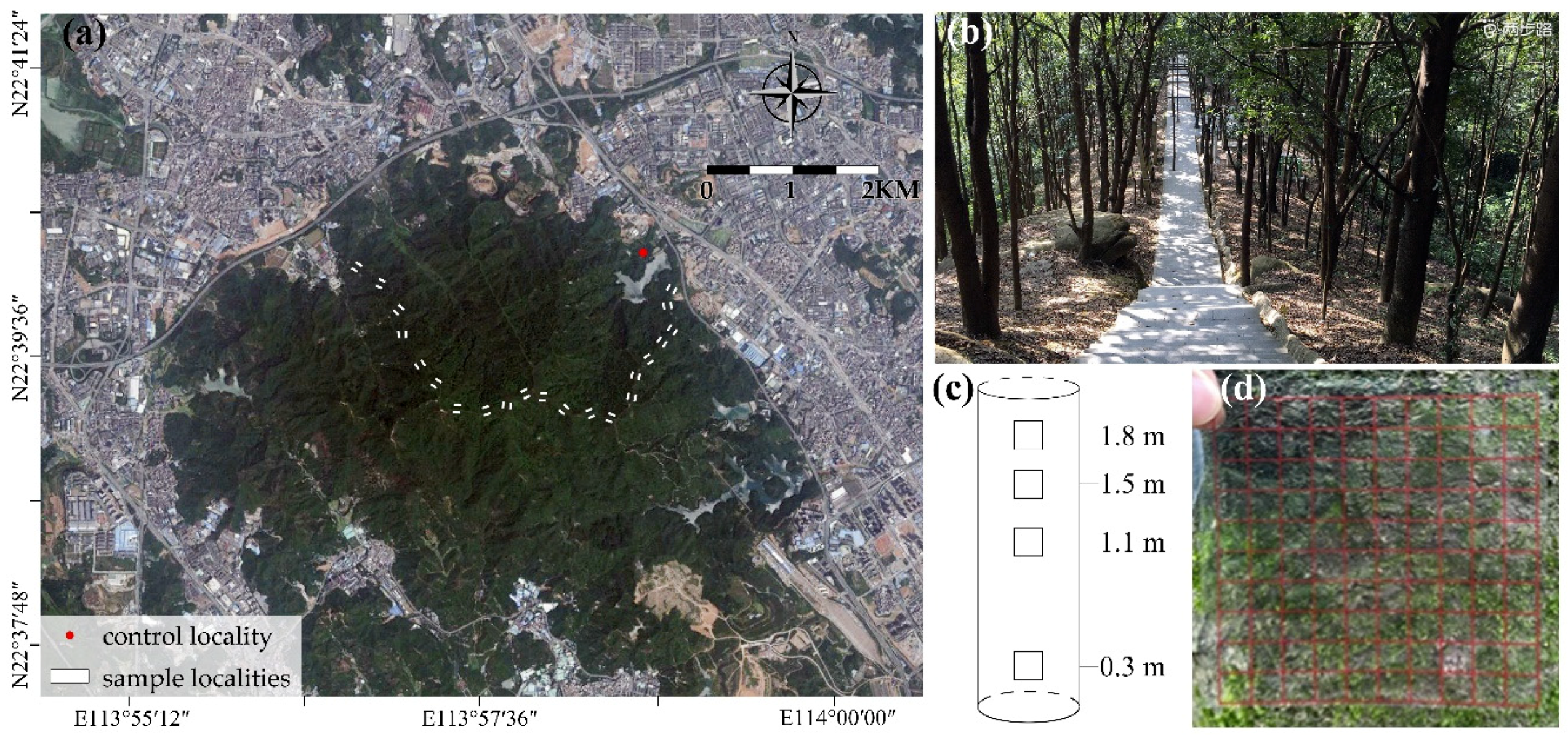
2.2. Site Selection
2.3. Bryophytes Data Collection
2.4. Environmental Data Collection
2.5. Data Analysis
3. Results
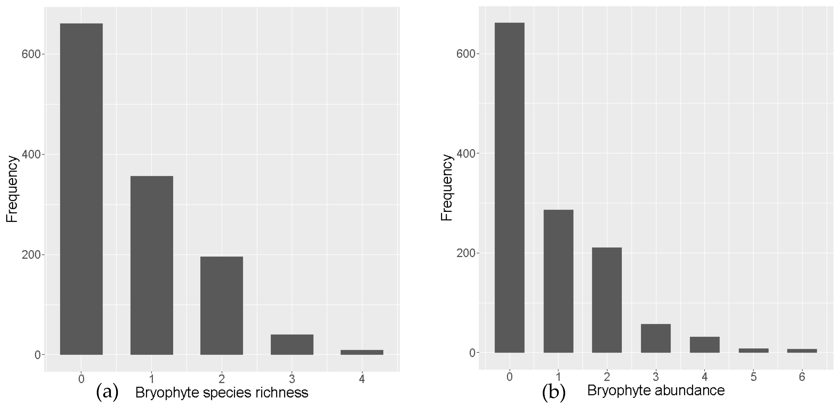
3.1. Overall Species Diversity and Distribution
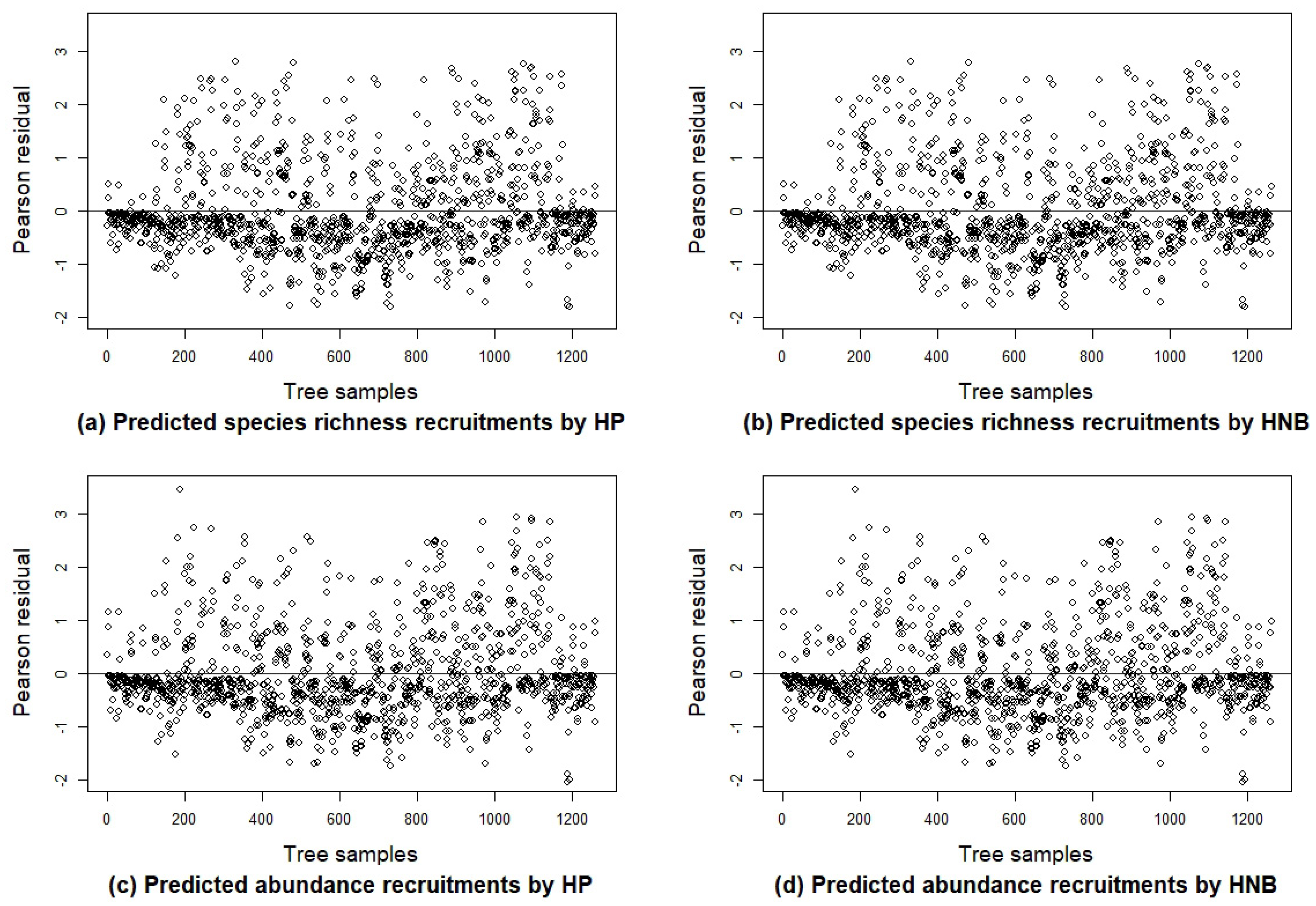
3.2. Species Richness Recruitment Models
3.3. Abundance Recruitment Models
4. Discussion
4.1. Overall Species Diversity and Distribution
4.2. Factors Affecting Epiphytic Bryophyte Recruitment
4.3. Comparison Among Basic Recruitment Models
5. Conclusions and Suggestions
Author Contributions
Funding
Acknowledgments
Conflicts of Interest
Appendix A


| NO. | Species | Frequency (Tree) | Frequency (Subplot) | Bryophyte Coverage (cm2) |
|---|---|---|---|---|
| 1 | Sematophyllum subhumile (Müll. Hal.) M. Fleisch. | 351 | 1315 | 14,847 |
| 2 | Pylaisiadelpha yokohamae (Broth.) W.R. Buck | 293 | 1028 | 12,199 |
| 3 | Lejeunea anisophylla Mont. | 162 | 573 | 2799 |
| 4 | Cololejeunea planissima (Mitt.) Abeyw. | 41 | 83 | 242 |
| 5 | Campylopus japonicus Broth. | 12 | 23 | 87 |
| 6 | Fissidens minutus Thwaites & Mitt. | 10 | 11 | 36 |
| 7 | Lejeunea ulicina (Taylor) Gottsche, Lindenb. & Nees | 9 | 10 | 26 |
| 8 | Cheilolejeunea ryukyuensis Mizut. | 5 | 6 | 16 |
| 9 | Metzgeria furcata (L.) Corda | 3 | 3 | 20 |
| 10 | Sematophyllum phoeniceum (Müll. Hal.) M. Fleisch. | 3 | 10 | 32 |
| 11 | Frullania muscicola Steph. | 3 | 3 | 17 |
| 12 | Fissidens crispulus Brid. | 2 | 2 | 4 |
| 13 | Pseudotaxiphyllum pohliaecarpum (Sull. & Lesq.) Z. Iwats. | 2 | 2 | 4 |
| 14 | Isopterygium minutirameum (Müll. Hal.) A. Jaeger | 2 | 2 | 5 |
| 15 | Lejeunea flava (Sw.) Nees | 1 | 2 | 11 |
| 16 | Ectropothecium buitenzorgi (Bél.) Mitt. | 1 | 1 | 4 |
| 17 | Entodon macropodus (Hedw.) Müll. Hal. | 1 | 1 | 2 |
| H | HB | DBH | CW | LAI | CD | ALT | NI | SLP | IHA | RT | RH |
|---|---|---|---|---|---|---|---|---|---|---|---|
| Before screening variables | |||||||||||
| 2.07 | 1.15 | 2.28 | 1.95 | 29.87 | 31.87 | 14.76 | 1.30 | 1.30 | 1.60 | 34.54 | 14.38 |
| After screening variables | |||||||||||
| 2.03 | 1.12 | 2.26 | 1.90 | 1.50 | - | 2.07 | 1.13 | 1.17 | 1.51 | - | - |
| H | HB | DBH | CW | LAI | CD | ALT | NI | SLP | IHA | RT | RH | |
|---|---|---|---|---|---|---|---|---|---|---|---|---|
| H | 1 | 0.15** | 0.67** | 0.44** | 0.05 | 0.04 | 0.15** | 0.03 | −0.16** | −0.14** | −0.17** | 0.18** |
| HB | 1 | −0.03 | −0.10** | −0.04 | −0.02 | −0.03 | 0.10** | −0.13** | −0.03 | 0.04 | −0.05 | |
| DBH | 1 | 0.60** | −0.02 | −0.02 | 0.004 | 0.02 | −0.07* | −0.07** | 0.001 | 0.01 | ||
| CW | 1 | −0.14** | −0.13** | −0.25** | 0.04 | 0.001 | 0.12** | 0.27** | −0.27** | |||
| LAI | 1 | 0.98** | 0.63** | 0.02 | −0.09** | −0.24** | −0.53** | 0.53** | ||||
| CD | 1 | 0.64** | 0.04 | −0.11** | −0.23** | −0.53** | 0.52** | |||||
| ALT | 1 | 0.03 | −0.19** | −0.43** | −0.96** | 0.94** | ||||||
| NI | 1 | −0.24** | −0.28** | 0.04 | −0.05 | |||||||
| SLP | 1 | 0.34** | 0.18** | −0.07** | ||||||||
| IHA | 1 | 0.52** | −0.50** | |||||||||
| RT | 1 | −0.98** | ||||||||||
| RH | 1 |
References
- Smith, A.J.E. Epiphytes and Epiliths. In Bryophyte Ecology; Smith, A.J.E., Ed.; Springer: Berlin, Germany, 1982; pp. 191–227. [Google Scholar]
- Ah-Peng, C.; Cardoso, A.W.; Flores, O.; West, A.; Wilding, N.; Strasberg, D.; Hedderson, T.A.J. The role of epiphytic bryophytes in interception, storage, and the regulated release of atmospheric moisture in a tropical montane cloud forest. J. Hydrol. 2017, 548, 665–673. [Google Scholar] [CrossRef]
- Lindo, Z.; Whiteley, J.A. Old trees contribute bio-available nitrogen through canopy bryophytes. Plant Soil 2011, 342, 141–148. [Google Scholar] [CrossRef]
- Glime, J.M. The fauna: A place to call home. Chapt. 1. In Bryophyte Ecology; Glime, J.M., Ed.; Michigan Technological University and International Association of Bryologists: Houghton, MI, USA, 2017. [Google Scholar]
- Oishi, Y.; Hiura, T. Bryophytes as bioindicators of the atmospheric environment in urban-forest landscapes. Landsc. Urban Plan. 2017, 167, 348–355. [Google Scholar] [CrossRef]
- Chen, H.Y.H.; Légaré, S.; Bergeron, Y. Variation of the understory composition and diversity along a gradient of productivity in Populus tremuloides stands of northern British Columbia, Canada. Can. J. Bot. 2004, 82, 1314–1323. [Google Scholar] [CrossRef]
- Ódor, P.; Király, I.; Tinya, F.; Bortignon, F.; Nascimbene, J. Reprint of: Patterns and drivers of species composition of epiphytic bryophytes and lichens in managed temperate forests. For. Ecol. Manag. 2014, 321, 42–51. [Google Scholar] [CrossRef]
- Zotz, G.; Bader, M.Y. Epiphytic Plants in a Changing World-Global: Change Effects on Vascular and Non-Vascular Epiphytes. In Progress in Botany; Lüttge, U., Beyschlag, W., Büdel, B., Francis, D., Eds.; Springer: Berlin, Germany, 2008; pp. 147–170. ISBN 978-3-540-68420-6. [Google Scholar]
- Oliveira, J.R.P.M.; Pôrto, K.C.; Silva, M.P.P. Richness preservation in a fragmented landscape: A study of epiphytic bryophytes in an Atlantic forest remnant in northeast Brazil. J. Bryol. 2011, 33, 279–290. [Google Scholar] [CrossRef]
- Edman, M.; Eriksson, A.M.; Villard, M.A. The importance of large-tree retention for the persistence of old-growth epiphytic bryophyte Neckera pennata in selection harvest systems. For. Ecol. Manag. 2016, 372, 143–148. [Google Scholar] [CrossRef]
- Benýtez, A.; Prieto, M.; Aragon, G. Large trees and dense canopies: Key factors for maintaining high epiphytic diversity on trunk bases (bryophytes and lichens) in tropical montane forests. Forestry 2014, 88, 521–527. [Google Scholar] [CrossRef] [Green Version]
- Fritz, Ö.; Heilmann-Clausen, J. Rot holes create key microhabitats for epiphytic lichens and bryophytes on beech (Fagus sylvatica). Biol. Conserv. 2010, 143, 1008–1016. [Google Scholar] [CrossRef]
- Boudreault, C.; Gauthier, S.; Bergeron, Y. Epiphytic Lichens and Bryophytes on Populus tremuloides Along a Chronosequence in the Southwestern Boreal Forest of Québec, Canada. Bryologist 2000, 103, 725–738. [Google Scholar] [CrossRef]
- Király, I.; Ódor, P. The effect of stand structure and tree species composition on epiphytic bryophytes in mixed deciduous-coniferous forests of Western Hungary. Biol. Conserv. 2010, 143, 2063–2069. [Google Scholar] [CrossRef]
- Zartman, C.E. Habitat fragmentation impacts on epiphyllous bryophyte communities in central Amazonia. Ecology 2003, 84, 948–954. [Google Scholar] [CrossRef]
- McGee, G.G.; Kimmerer, R.W. Forest age and management effects on epiphytic bryophyte communities in Adirondack northern hardwood forests, New York, U.S.A. Can. J. For. Res. 2002, 32, 1562–1576. [Google Scholar] [CrossRef]
- Ojala, E.; Mönkkönen, M.; Inkeröinen, J. Epiphytic bryophytes on European aspen Populus tremula in old-growth forests in northeastern Finland and in adjacent sites in Russia. Can. J. Bot. 2000, 78, 529–536. [Google Scholar]
- Tuba, Z.; Slack, N.G.; Stark, L.R.; Jácome, J.; Gradstein, S.R.; Kessler, M.; Tuba, Z.; Slack, N.G.; Stark, L.R. Responses of Epiphytic Bryophyte Communities to Simulated Climate Change in the Tropics. In Bryophyte Ecology and Climate Change; Tuba, Z., Slack, N.G., Stark, L.R., Eds.; Cambridge University Press: Cambridge, UK, 2012; pp. 191–208. [Google Scholar]
- Song, L.; Liu, W.; Zhang, Y.; Tan, Z.; Li, S.; Qi, J.; Yao, Y. Assessing the Potential Impacts of Elevated Temperature and CO2 on Growth and Health of Nine Non-Vascular Epiphytes: A Manipulation Experiment. Am. J. Plant Sci. 2014, 5, 1587–1598. [Google Scholar] [CrossRef] [Green Version]
- Mitchell, R.J.; Sutton, M.A.; Truscott, A.M.; Leith, I.D.; Cape, J.N.; Pitcairn, C.E.R.; Van Dijk, N. Growth and tissue nitrogen of epiphytic Atlantic bryophytes: Effects of increased and decreased atmospheric N deposition. Funct. Ecol. 2004, 18, 322–329. [Google Scholar] [CrossRef]
- Coker, P.D. The effects of sulphur dioxide pollution on bark epiphytes. Trans. Br. Bryol. Soc. 1967, 5, 341–347. [Google Scholar] [CrossRef]
- Newbold, T.; Hudson, L.N.; Hill, S.L.L.; Contu, S.; Lysenko, I.; Senior, R.A.; Börger, L.; Bennett, D.J.; Choimes, A.; Collen, B.; et al. Global effects of land use on local terrestrial biodiversity. Nature 2015, 520, 45–50. [Google Scholar] [CrossRef] [Green Version]
- Oishi, Y. Urban heat island effects on moss gardens in Kyoto, Japan. Landsc. Ecol. Eng. 2019, 15, 177–184. [Google Scholar] [CrossRef]
- Spagnuolo, V.; De Nicola, F.; Terracciano, S.; Bargagli, R.; Baldantoni, D.; Monaci, F.; Alfani, A.; Giordano, S. Persistent pollutants and the patchiness of urban green areas as drivers of genetic richness in the epiphytic moss Leptodon smithii. J. Environ. Sci. 2014, 26, 2493–2499. [Google Scholar] [CrossRef]
- Bhatt, A.; Gairola, S.; Govender, Y.; Baijnath, H.; Ramdhani, S. Epiphyte diversity on host trees in an urban environment, eThekwini Municipal Area, South Africa. N. Z. J. Bot. 2015, 53, 24–37. [Google Scholar] [CrossRef]
- Sérgio, C.; Carvalho, P.; Garcia, C.A.; Almeida, E.; Novais, V.; Sim-Sim, M.; Jordão, H.; Sousa, A.J. Floristic changes of epiphytic flora in the Metropolitan Lisbon area between 1980–1981 and 2010–2011 related to urban air quality. Ecol. Indic. 2016, 67, 839–852. [Google Scholar] [CrossRef]
- Larsen, R.S.; Bell, J.N.B.; James, P.W.; Chimonides, P.J.; Rumsey, F.J.; Tremper, A.; Purvis, O.W. Lichen and bryophyte distribution on oak in London in relation to air pollution and bark acidity. Environ. Pollut. 2007, 146, 332–340. [Google Scholar] [CrossRef] [PubMed]
- Moskell, C.; Allred, S.B. Residents’ beliefs about responsibility for the stewardship of park trees and street trees in New York City. Landsc. Urban Plan. 2013, 120, 85–95. [Google Scholar] [CrossRef]
- Imam, A.U.K.; Banerjee, U.K. Urbanisation and greening of Indian cities: Problems, practices, and policies. Ambio 2016, 45, 442–457. [Google Scholar] [CrossRef] [Green Version]
- Yang, J.; Jinxing, Z. The failure and success of greenbelt program in Beijing. Urban For. Urban Green. 2007, 6, 287–296. [Google Scholar] [CrossRef]
- Baker, T.P.; Jordan, G.J.; Fountain-Jones, N.M.; Balmer, J.; Dalton, P.J.; Baker, S.C. Distance, environmental and substrate factors impacting recovery of bryophyte communities after harvesting. Appl. Veg. Sci. 2018, 21, 64–75. [Google Scholar] [CrossRef]
- Medina, N.G.; Bowker, M.A.; Hortal, J.; Mazimpaka, V.; Lara, F. Shifts in the importance of the species pool and environmental controls of epiphytic bryophyte richness across multiple scales. Oecologia 2018, 186, 805–816. [Google Scholar] [CrossRef] [PubMed]
- Patiño, J.; Gómez-Rodríguez, C.; Pupo-Correia, A.; Sequeira, M.; Vanderpoorten, A. Trees as habitat islands: Temporal variation in alpha and beta diversity in epiphytic laurel forest bryophyte communities. J. Biogeogr. 2018, 45, 1727–1738. [Google Scholar] [CrossRef]
- Turner, P.A.M.; Kirkpatrick, J.B.; Pharo, E.J. Bryophyte relationships with environmental and structural variables in Tasmanian old-growth mixed eucalypt forest. Aust. J. Bot. 2006, 54, 239–247. [Google Scholar] [CrossRef]
- Zhang, X.; Lei, Y.; Cai, D.; Liu, F. Predicting tree recruitment with negative binomial mixture models. For. Ecol. Manag. 2012, 270, 209–215. [Google Scholar] [CrossRef]
- Woollons, R.C. Even-aged stand mortality estimation through a two-step regression process. For. Ecol. Manag. 1998, 105, 189–195. [Google Scholar] [CrossRef]
- Diéguez-Aranda, U.; Castedo-Dorado, F.; Álvarez-González, J.G.; Rodríguez-Soalleiro, R. Modelling mortality of Scots pine (Pinus sylvestris L.) plantations in the northwest of Spain. Eur. J. For. Res. 2005, 124, 143–153. [Google Scholar] [CrossRef]
- Levin, K.A.; Davies, C.A.; Topping, G.V.A.; Assaf, A.V.; Pitts, N.B. Inequalities in dental caries of 5-year-old children in Scotland, 1993–2003. Eur. J. Public Health 2009, 19, 337–342. [Google Scholar] [CrossRef] [Green Version]
- Czado, C.; Gneiting, T.; Held, L. Predictive model assessment for count data. Biometrics 2009, 65, 1254–1261. [Google Scholar] [CrossRef] [PubMed]
- Bilgic, A.; Florkowski, W.J. Application of a hurdle negative binomial count data model to demand for bass fishing in the southeastern United States. J. Environ. Manag. 2007, 83, 478–490. [Google Scholar] [CrossRef]
- Marchal, J.; Cumming, S.G.; McIntire, E.J.B. Exploiting Poisson additivity to predict fire frequency from maps of fire weather and land cover in boreal forests of Québec, Canada. Ecography (Cop.) 2017, 40, 200–209. [Google Scholar] [CrossRef] [Green Version]
- Su, Z.; Tigabu, M.; Cao, Q.; Wang, G.; Hu, H.; Guo, F. Comparative analysis of spatial variation in forest fire drivers between boreal and subtropical ecosystems in China. For. Ecol. Manag. 2019, 454, 117669. [Google Scholar] [CrossRef]
- Shenzhen Climate Bulletin in 2018. Available online: http://weather.sz.gov.cn/qixiangfuwu/qihoufuwu/qihouguanceyupinggu/nianduqihougongbao/201901/t20190116_15306885.htm (accessed on 24 January 2020).
- Chen, Y.; Sun, B.; Liao, S.B.; Chen, L.; Luo, S.X. Landscape perception based on personal attributes in determining the scenic beauty of in-stand natural secondary forests. Ann. For. Res. 2016, 59, 91–103. [Google Scholar] [CrossRef] [Green Version]
- González-Montelongo, C.; Pérez-Vargas, I. Looking for a home: Exploring the potential of epiphytic lichens to colonize tree plantations in a Macaronesian laurel forest. For. Ecol. Manag. 2019, 453, 117541. [Google Scholar] [CrossRef]
- Ministry of Ecology and Environment. Technical Guidelines for Boidiversity Monitoring-Lichens and Bryophytes (HJ 710.2-2014); China Environmental Science Press: Beijing, China, 2015. (In Chinese)
- Wu, D.L.; Zhang, L. Bryophyte flora of Guangdong; Guangdong Science and Technology Press: Guangzhou, China, 2013. (In Chinese) [Google Scholar]
- Zhang, L. An updated and annotated inventory of Hong Kong bryophytes. Mem. Hong Kong Nat. Hist. Soc. 2003, 26, 1–133. [Google Scholar]
- Glime, J.M.; Hong, W.S. Bole Epiphytes on Three Conifer Species from Queen Charlotte Islands, Canada. Bryologist 2002, 105, 451–464. [Google Scholar] [CrossRef]
- Oishi, Y. Influence of urban green spaces on the conservation of bryophyte diversity: The special role of Japanese gardens. Landsc. Urban Plan. 2012, 106, 6–11. [Google Scholar] [CrossRef] [Green Version]
- Bergamini, A.; Stofer, S.; Bolliger, J.; Scheidegger, C. Evaluating macrolichens and environmental variables as predictors of the diversity of epiphytic microlichens. Lichenologist 2007, 39, 475–489. [Google Scholar] [CrossRef] [Green Version]
- Ferguson, D.E.; Stage, A.R.; Boyd, R.J. Predicting regeneration in the grand fir- cedar- hemlock ecosystem of the northern Rocky Mountains. For. Sci. Monogr. 1986, 26, a0001–z0001. [Google Scholar]
- Xiang, W.; Lei, X.; Zhang, X. Modelling tree recruitment in relation to climate and competition in semi-natural Larix-Picea-Abies forests in northeast China. For. Ecol. Manag. 2016, 382, 100–109. [Google Scholar] [CrossRef]
- Fernández-Alonso, M.J.; Díaz-Pinés, E.; Ortiz, C.; Rubio, A. Disentangling the effects of tree species and microclimate on heterotrophic and autotrophic soil respiration in a Mediterranean ecotone forest. For. Ecol. Manag. 2018, 430, 533–544. [Google Scholar] [CrossRef] [Green Version]
- Venables, W.N.; Ripley, B.D. Statistics Complements to Modern Applied Statistics with S-Plus by. In Compare A Journal Of Comparative Education; Venables, W.N., Ripley, B.D., Eds.; Springer: Berlin, Germany, 1999; ISBN 0387982140. [Google Scholar]
- Guthery, F.S.; Burnham, K.P.; Anderson, D.R. Model Selection and Multimodel Inference: A Practical Information-Theoretic Approach; Springer: New York, NY, USA, 2003; Volume 67. [Google Scholar]
- Vuong, Q.H. Likelihood Ratio Tests for Model Selection and Non-Nested Hypotheses. Econometrica 1989, 57, 307. [Google Scholar] [CrossRef] [Green Version]
- Colin, C.A.; Pravin, T. Regression Analysis of Count Data, 2nd ed.; Cambridge University Press: Cambridge, UK, 2013; ISBN 9781139013567. [Google Scholar]
- R Development Core Team. R: A Language and Environment for Statistical Computing; R Development Core Team: Vienna, Austria, 2019. [Google Scholar]
- Anderson, D.R. Model Based Inference in the Life Sciences: A Primer on Evidence; Springer Science & Business Media: New York, NY, USA, 2008; ISBN 9780387740737. [Google Scholar]
- Liu, W.Q.; Dai, X.H.; Wang, Y.F.; Lei, C.Y. Analysis of environmental factors affecting the distribution of epiphytic bryophyte at Heishiding Nature Reserve, Guangdong Province. Acta Ecol. Sin. 2008, 28, 1080–1088. (In Chinese) [Google Scholar]
- Thomas, S.C.; Liguori, D.A.; Halpern, C.B. Corticolous bryophytes in managed Douglas-fir forests: Habitat differentiation and responses to thinning and fertilization. Can. J. Bot. 2001, 79, 886–896. [Google Scholar]
- Dislich, R.; Pinheiro, E.M.L.; Guimarães, M. Corticolous liverworts and mosses in a gallery forest in central Brazil: Effects of environmental variables and space on species richness and composition. Nov. Hedwig. 2018, 107, 385–406. [Google Scholar] [CrossRef]
- Romanski, J.; Pharo, E.J.; Kirkpatrick, J.B. Epiphytic bryophytes and habitat variation in montane rainforest, Peru. Bryologist 2012, 114, 720. [Google Scholar] [CrossRef]
- Marschall, M.; Proctor, M.C.F. Are bryophytes shade plants? Photosynthetic light responses and proportions of chlorophyll a, chlorophyll b and total carotenoids. Ann. Bot. 2004, 94, 593–603. [Google Scholar] [CrossRef] [PubMed] [Green Version]
- Romanski, J. Epiphytic Bryophytes and Habitat Microclimate Variation in Lower Montane Rainforest, Peru; University of Tasmania: Hobart, Australia, 2013. [Google Scholar]
- Franks, A.J.; Bergstrom, D.M. Corticolous bryophytes in microphyll fern forests of south-east Queensland: Distribution on Antarctic beech (Nothofagus moorei). Austral Ecol. 2000, 25, 386–393. [Google Scholar] [CrossRef]
- Fritz, Ö.; Brunet, J. Epiphytic bryophytes and lichens in Swedish beech forests—effects of forest history and habitat quality. Ecol. Bull. 2010, 95–108. [Google Scholar]
- Zotz, G.; Vollrath, B. The epiphyte vegetation of the palm Socratea exorrhiza-Correlations with tree size, tree age and bryophyte cover. J. Trop. Ecol. 2003, 19, 81–90. [Google Scholar] [CrossRef] [Green Version]
- Yan, X.; Bao, W.; Pang, X. Indirect effects of hiking trails on the community structure and diversity of trunkepiphytic bryophytes in an old-growth fir forest. J. Bryol. 2014, 36, 44–55. [Google Scholar] [CrossRef] [Green Version]
- Kantvilas, G.; Jarman, S.J. Lichens and bryophytes on Eucalyptus obliqua in Tasmania: Management implications in production forests. Biol. Conserv. 2004, 117, 359–373. [Google Scholar] [CrossRef]
- Fritz, Ö.; Niklasson, M.; Churski, M. Tree age is a key factor for the conservation of epiphytic lichens and bryophytes in beech forests. Appl. Veg. Sci. 2009, 12, 93–106. [Google Scholar] [CrossRef]
- Werner, F.A.; Gradstein, S.R. Diversity of dry forest epiphytes along a gradient of human disturbance in the tropical andes. J. Veg. Sci. 2009, 20, 59–68. [Google Scholar] [CrossRef]
- Wolf, J.H.D. Diversity Patterns and Biomass of Epiphytic Bryophytes and Lichens Along an Altitudinal Gradient in the Northern Andes. Ann. Missouri Bot. Gard. 1993, 80, 928. [Google Scholar] [CrossRef]
- Song, L.; Ma, W.Z.; Yao, Y.L.; Liu, W.Y.; Li, S.; Chen, K.; Lu, H.Z.; Cao, M.; Sun, Z.H.; Tan, Z.H.; et al. Bole bryophyte diversity and distribution patterns along three altitudinal gradients in Yunnan, China. J. Veg. Sci. 2015, 26, 576–587. [Google Scholar] [CrossRef]
- Mežaka, A.; Znotiņa, V.; Piterāns, A. Distribution of Epiphytic Bryophytes in Five Latvian Natural Forest Stands of Slopes, Screes and Ravines. Acta Biol. Univ. Daugavpil 2005, 5, 101–108. [Google Scholar]
- Richter, S.; Schütze, P.; Bruelheide, H. Modelling epiphytic bryophyte vegetation in an urban landscape. J. Bryol. 2009, 31, 159–168. [Google Scholar] [CrossRef]
- Zeileis, A.; Kleiber, C.; Jackman, S. Regression models for count data in R. J. Stat. Softw. 2008, 27, 1–25. [Google Scholar] [CrossRef] [Green Version]
- Eskelson, B.N.I.; Temesgen, H.; Barrett, T.M. Estimating cavity tree and snag abundance using negative binomial regression models and nearest neighbor imputation methods. Can. J. For. Res. 2009, 39, 1749–1765. [Google Scholar] [CrossRef] [Green Version]
- Mullahy, J. Specification and testing of some modified count data models. J. Econom. 1986, 33, 341–365. [Google Scholar] [CrossRef]

| Variable | Unit | Mean | S. E. | Min. | Max. |
|---|---|---|---|---|---|
| Response variables | |||||
| Species richness | 0.72 | 0.89 | 0 | 4 | |
| Abundance | 0.86 | 1.15 | 0 | 6 | |
| Tree characteristics | |||||
| H | m | 10.43 | 1.75 | 6.00 | 15.10 |
| HB | m | 3.65 | 1.85 | 0.20 | 10.30 |
| DBH | cm | 18.72 | 5.52 | 10.00 | 38.60 |
| CW | m | 3.61 | 1.14 | 1.80 | 7.30 |
| Stand characteristics | |||||
| LAI | 2.63 | 0.63 | 1.48 | 3.85 | |
| CD | % | 84.12 | 8.88 | 63.10 | 96.95 |
| Terrain factors | |||||
| ALT | m | 363.38 | 122.36 | 153.50 | 534.00 |
| NI | 0.21 | 0.64 | -0.98 | 1.00 | |
| SLP | ° | 14.55 | 6.74 | 2.00 | 30.00 |
| Microclimate | |||||
| RT | 0.86 | 0.04 | 0.80 | 0.93 | |
| RH | 1.25 | 0.06 | 1.14 | 1.35 | |
| Human effects | |||||
| IHA | 0.42 | 0.24 | 0.04 | 1.00 | |
| Parameter | Poisson Estimation | NB Estimation | ZIP Estimation | ZINB Estimation | HP Estimation | HNB Estimation |
|---|---|---|---|---|---|---|
| Positive count component of the model | ||||||
| Intercept | −8.3688*** (0.7395) | −8.3692*** (0.7395) | −2.5316*** (0.3625) | −2.5316*** (0.3625) | −1.9287*** (0.3590) | −1.9288*** (0.3590) |
| H | 0.1947*** (0.0285) | 0.1947*** (0.0285) | 0.0974** (0.0310) | 0.0974** (0.0310) | ||
| HB | −0.0487* (0.0193) | −0.0487* (0.0193) | −0.0578** (0.0191) | −0.0578** (0.0191) | ||
| DBH | 0.0663*** (0.0071) | 0.0664*** (0.0071) | 0.0442*** (0.0072) | 0.0442*** (0.0072) | 0.0537*** (0.0089) | 0.0537*** (0.0089) |
| LAI | 0.6712*** (0.1718) | 0.6712*** (0.1718) | 0.7505*** (0.1481) | 0.7505*** (0.1481) | 0.5749* (0.2407) | 0.5754* (0.2408) |
| ALT | 0.7302*** (0.1308) | 0.7302*** (0.1308) | ||||
| SLP | −0.0180** (0.0059) | −0.0180** (0.0059) | ||||
| Log(theta) | 9.3268 (10.7522) | 16.5353 (8.6607) | 12.2713 (77.6908) | |||
| Zero component of the model | ||||||
| Intercept | 69.0494*** (11.8525) | 69.0436*** (11.8505) | −21.8672*** (1.8696) | −21.8672*** (1.8696) | ||
| H | −1.0245*** (0.2328) | −1.0244*** (0.2328) | 0.5972*** (0.0706) | 0.5972*** (0.0706) | ||
| HB | −0.1432*** (0.0428) | −0.1432*** (0.0428) | ||||
| DBH | −0.7510*** (0.1380) | −0.7509*** (0.1379) | 0.2464*** (0.0245) | 0.2464*** (0.0245) | ||
| LAI | 2.2049*** (0.3898) | 2.2049*** (0.3898) | ||||
| ALT | −8.3747*** (1.5548) | −8.3739*** (1.5546) | 1.7055*** (0.2908) | 1.7055*** (0.2908) | ||
| NI | −1.2398** (0.4538) | −1.2397** (0.4538) | ||||
| IHA | 3.6473** (1.1690) | 3.6472** (1.1689) | −1.4274*** (0.3786) | −1.4274*** (0.3786) | ||
| AIC | 2337.4 | 2339.4 | 2176.156 | 2178.156 | 2091.495 | 2093.496 |
| Parameter | Poisson Estimation | NB Estimation | ZIP Estimation | ZINB Estimation | HP Estimation | HNB Estimation |
|---|---|---|---|---|---|---|
| Positive count component of the model | ||||||
| Intercept | −11.6241*** (0.8485) | −11.6248*** (0.8486) | −7.4538*** (0.9531) | −7.4524*** (0.9531) | −16.8285*** (1.5735) | −16.8224*** (1.5733) |
| H | 0.1820*** (0.0267) | 0.1820*** (0.0267) | ||||
| HB | −0.0452** (0.0175) | −0.0452** (0.0175) | ||||
| DBH | 0.0622*** (0.0068) | 0.0622*** (0.0068) | 0.0543*** (0.0062) | 0.0543*** (0.0062) | 0.0497*** (0.0077) | 0.0497*** (0.0077) |
| LAI | 0.8560*** (0.1714) | 0.8561*** (0.1714) | 0.8683*** (0.1753) | 0.8684*** (0.1753) | ||
| ALT | 1.3460*** (0.1457) | 1.3460*** (0.1458) | 0.9961*** (0.1622) | 0.9959*** (0.1622) | 2.6901*** (0.2476) | 2.6891*** (0.2475) |
| SLP | −0.0261*** (0.0056) | −0.0261*** (0.0056) | −0.01944*** (0.0055) | −0.0194*** (0.0055) | −0.0219** (0.0075) | −0.0219** (0.0075) |
| IHA | −0.3344* (0.1494) | −0.3344* (0.1494) | ||||
| Log(theta) | 15.7752 (23.7270) | 11.9638 (55.9250) | ||||
| Zero component of the model | ||||||
| Intercept | 33.8386*** (5.7331) | 33.8625*** (5.7372) | −21.8672*** (1.8696) | −21.8672*** (1.8696) | ||
| H | −1.1304*** (0.1987) | −1.1309*** (0.1988) | 0.5972*** (0.0706) | 0.5972*** (0.0706) | ||
| HB | 0.3445*** (0.1016) | 0.3447*** (0.1016) | −0.1432*** (0.0428) | −0.1432*** (0.0428) | ||
| DBH | −0.4194*** (0.0756) | −0.4195*** (0.0756) | 0.2464*** (0.0245) | 0.2464*** (0.0245) | ||
| LAI | 2.2049*** (0.3898) | 2.2049*** (0.3898) | ||||
| ALT | −3.2089*** (0.7701) | −3.2121*** (0.7706) | 1.7055*** (0.2908) | 1.7055*** (0.2908) | ||
| IHA | 3.1691*** (0.8507) | 3.1698*** (0.8510) | −1.4274*** (0.3786) | −1.4274*** (0.3786) | ||
| AIC | 2534.2 | 2536.2 | 2385.514 | 2387.514 | 2285.192 | 2287.193 |
© 2020 by the authors. Licensee MDPI, Basel, Switzerland. This article is an open access article distributed under the terms and conditions of the Creative Commons Attribution (CC BY) license (http://creativecommons.org/licenses/by/4.0/).
Share and Cite
Zhao, D.; Sun, Z.; Wang, C.; Hao, Z.; Sun, B.; Zuo, Q.; Duan, W.; Bian, Q.; Bai, Z.; Wei, K.; et al. Using Count Data Models to Predict Epiphytic Bryophyte Recruitment in Schima superba Gardn. et Champ. Plantations in Urban Forests. Forests 2020, 11, 174. https://doi.org/10.3390/f11020174
Zhao D, Sun Z, Wang C, Hao Z, Sun B, Zuo Q, Duan W, Bian Q, Bai Z, Wei K, et al. Using Count Data Models to Predict Epiphytic Bryophyte Recruitment in Schima superba Gardn. et Champ. Plantations in Urban Forests. Forests. 2020; 11(2):174. https://doi.org/10.3390/f11020174
Chicago/Turabian StyleZhao, Dexian, Zhenkai Sun, Cheng Wang, Zezhou Hao, Baoqiang Sun, Qin Zuo, Wenjun Duan, Qi Bian, Zitong Bai, Kaiyue Wei, and et al. 2020. "Using Count Data Models to Predict Epiphytic Bryophyte Recruitment in Schima superba Gardn. et Champ. Plantations in Urban Forests" Forests 11, no. 2: 174. https://doi.org/10.3390/f11020174