Object Detection of Ground-Penetrating Radar Signals Using Empirical Mode Decomposition and Dynamic Time Warping


1
School of IoT Engineering, Jiangnan University, Wuxi 214122, China
2
USDA Forest Products Laboratory, Madison, WI 53726, USA
*
Author to whom correspondence should be addressed.
Forests 2020, 11(2), 230; https://doi.org/10.3390/f11020230
Submission received: 8 January 2020
/
Revised: 4 February 2020
/
Accepted: 15 February 2020
/
Published: 19 February 2020
(This article belongs to the Section Wood Science and Forest Products)
Abstract
:An object detection method of ground-penetrating radar (GPR) signals using empirical mode decomposition (EMD) and dynamic time warping (DTW) is proposed in this study. Two groups of timber specimens were examined. The first group comprised of Douglas fir (Pseudotsuga menziesii) timber sections prepared in the laboratory with inserts of known internal characteristics. The second group comprised of timber girders salvaged from the timber bridges on historic Route 66 over 80 years. A GSSI Subsurface Interface Radar (SIR) System 4000 with a 2 GHz palm antenna was used to scan these two groups of specimens. GPR sensed differences in dielectric constants (DC) along the scan path caused by the presence of water, metal, or air within the wood. This study focuses on the feature identification and defect classification. The results show that the processing methods were efficient for the illustration of GPR information.

1. Introduction
Nondestructive testing (NDT) techniques are often applied to evaluate the internal condition of wood structures. Ground-penetrating radar (GPR) technology has been widely used for detecting buried objects of varied materials such as sand, timber, concrete, etc. It has been clearly illustrated that GPR can detect anomalous electromagnetic responses associated with a variety of significant physical conditions [1].
1.1. Description of Radar Wave Transmission and Reflection
GPR is a noninvasive geophysical technique for high-resolution imaging and characterization of subsurface media by means of transmitting and receiving high-frequency electromagnetic (EM) waves [2]. Annan explained the theory of GPR. Electromagnetic fields that propagate as essentially nondispersive waves were used to detect structures and the changes of material properties within the materials [3]. The waves emitted travels through the material are scattered and/or reflected by changes in impedance, giving rise to events similar to the emitted signal. The connection between dielectric permittivity and EM wave velocity (v) could be formulated by Equation (1). The variation of two-way travel time, amplitude, or/and frequency of reflection wave are measured by Equation (2) [4].
where vc is EM wave traveling velocity in free space and ε′ the real part of complex dielectric permittivity [5].
where w is two-way travel time of an EM pulse in structure members, H is measured depth to reflecting interface in structure members.
1.2. Brief Description of Other Studies Using the Method to Image Wood Defects
Schad et al. [6] investigated three nondestructive evaluation techniques for detecting internal wood defects. Both sound wave transmission and impulse radar were able to detect large voids and areas of degradation. The use of radar requires an experienced operator because of the difficulty of interpreting the data. Brashaw [7] studied the signal analyzing of the radar data in both the longitudinal direction (antenna front to back) and the transverse direction (antenna side to side). This research was designed to be an early assessment of the potential for using GPR to identify known defects in longitudinal timber bridge decks and slab spans. Based on their experiments, they provided more thoughts for future study in the GPR. The ground layers with different dielectric permittivity cause changes in the peak positions and the amplitudes of the reflected signal. Recorded radargrams are then analyzed to obtain information on the subsurface structure of timber structures [8]. GPR technique was well suited for the inspection of timber bridges. The observations were due essentially to the reflections of the electromagnetic wave on defects due to the modification of the permittivity contrast of the material between damaged and non-damaged wood [9,10]. The electromagnetic response of all the reflected waves could be processed and analyzed to estimate the propagation velocities or the depth of objects. The reflected wave of GPR has a direct relationship with the moisture content (MC) of wood. Martínez-Sala et al. [11] used GPR to assess physical properties of wood structures in situ. The results show that the propagation velocities and the amplitudes of the direct and reflected waves were lower when the electric field was parallel to the grain. Maï et al. [10] devoted to evaluate the timber structures based on the GPR technique. The resonance technique with a 1.26 GHz was selected to test the dielectric relative permittivity of spruce and pine wood samples. Then, they also used a GSSI SIR 3000 system with a 1.5-GHz antenna to test some wood samples. The whole data reflected the relationship between real/imaginary relative permittivity, the GPR features in time domains, and MC of the different wood samples. Hans et al. [12] investigated the MC of logs based on the propagation velocity of GPR signals. Linear regression between the log dielectric permittivity and MC was established for each of the investigated wood species (quaking aspen, balsam poplar, and black spruce), log state (thawed and frozen), and direction of measurement. Razafindratsima et al. [13] presented the measurements of relative permittivity values of spruce, pine, and beech wood samples over a wide range of moisture content (up to 120%) using weak perturbation method at 1.26 GHz. The results showed an increase in the real and imaginary parts of permittivity with the moisture content for all three wood species. Moreover, for considered moisture content, the relative permittivity corresponding to the electric field parallel to fiber direction was higher than when the electric field was perpendicular to the fiber direction.
The waveforms of one-dimensional data (A-Scan) and two-dimensional radargrams (B-Scan) contain information about the internal characteristics of the analyzed specimen. Xiang et al. [14] explained that the reflected wave produces hyperbolae, with the top of each hyperbola denoting the corresponding rebar position in the GPR images. Unfortunately, the waveforms also contain a variety of complex interference waves, increasing the difficulty of feature identification.
1.3. Breakdown of the Empirical Mode Decomposition (EMD) and Dynamic Time Warping (DTW) Methodology
In order to obtain high-quality signals, the noise level must be suppressed. One method of signal denoising is the empirical mode decomposition (EMD). EMD was proposed by Huang [15]. EMD method has been used in a broad variety of time-frequency analysis as well as signal processing [16]. It has the advantage to study the amplitude of the signal and to adaptively decompose the signal into stationary signal. The finite number of Intrinsic Mode Function (IMF) components decomposed represents the physical characteristic information of the signal. Battista et al. used EMD to remove cable strum noise from seismic data [17]. Narayanan et al. [18] used EMD to mitigate both coherent and random noise in wall radar human detection. Mallat [19] indicated that the window length determines the tradeoff between time and frequency resolution as the decomposition basis of sine and cosine waves can only provide a fixed spectral resolution. Bekara and Baan [20] used a new filtering technique for random and coherent noise attenuation in seismic data on constant-frequency slices in the frequency-offset _ f-x_ domain based on EMD. Zhu et al. [21] worked on identifying the multi-timescales of carbon market by a novel integrated model of grey relational analysis and EMD. They used grey relational analysis to examine the multi-timescales of carbon price and then chose EMD to decompose the carbon price into simpler components and tested the multi-timescales of each component using the random probability method. EMD provides scientific support for multiscale research in the carbon market.
Dynamic Time Warping (DTW) is a way to measure the similarity of two time series of different lengths. DTW is a typical optimization problem, and it uses the time-warping function to demonstrate time corresponding relation between a test template and a reference template. Warping one (or both) of the sequences in the timeline can achieve better alignment. Then, we can calculate the time warping function corresponding to the minimum cumulative distance between the two templates. DTW plays an important role in speech recognition and machine learning convenience. Jazayeri et al. [22] proposed a cutting-edge expert system by setting a threshold on DTW values and monitoring them online, and a significant deviation of the DTW values from the reference signal was detected prior to reaching an object. DTW algorithms align two signals in time dimension by creating a so-called “warping path” and determining a measure of their dissimilarity independent of certain non-linear variations [23]. Zhen et al. [24] used DTW to suppress the supply frequency component and highlight the sideband components by introducing a reference signal that has the same frequency component as that of the supply power. Moreover, a sliding window was designed to process the raw signal using DTW frame by frame for effective calculation. Parziale et al. [25] introduced the Stability Modulated Dynamic Time Warping algorithm for incorporating the stability regions on two datasets, i.e., the most similar parts between two signatures, into the distance measure between a pair of signatures computed by DTW for signature verification. The proposed algorithm improves the performance of the baseline system and is more favorable than other signature verification systems. The DTW distance can cope with temporal variations. Jain converted the DTW-distance to a warping-invariant semi-metric called time-warp-invariant (TWI) distance to eliminate the peculiarities. The final results of the tests indicated that the error rates of the TWI and DTW nearest-neighbor classifiers are practically equivalent in a Bayesian sense. Meanwhile, the required computation time and storage of TWI-distance sometimes were less than the DTW-distance. They suggested that the proposed TWI-distance was a more efficient and consistent option [26].
The hyperbolic waves in the Scan data reflected the difference of water, metal, or air, which has different DC. The purpose of this paper is to develop a new technique to recognize and locate the internal defects of wood structure. This study focuses on the feature identification and defect classification. A combined processing method using EMD and DTW was proposed on the GPR A-Scan data. The experimental results on ancient bridge timber demonstrated that the proposed method can help locate the internal defects successfully.
2. Materials
2.1. Theory of GPR Wave Propagation
GPR system is usually configured by at least one transmitting and one receiving antenna, a control unit, a data storage unit, and a display unit [27]. The antenna generated short bursts of electromagnetic energy in solid materials. The waveforms are transmitted into the structure using an antenna positioned at the surface [28]. A portion of the wave is reflected, refracted, and/or diffracted when encountering the boundary of objects with different DC and then is received by the antenna. Figure 1 illustrates the process of the creation of hyperbolic reflections for one target with the movement of the antenna.
2.2. Materials
In this study, we adopted two datasets from Douglas-fir (Pseudotsuga menziesii) timbers for experiments. One was derived from a project on the ancient bridge timber. This project focused on evaluating the ancient highway timber bridges located on the historic U.S. Route 66 in Southern California. This stretch of historic Route 66 in the Mojave Desert is currently the focus of extensive efforts by the County of San Bernardino to preserve its iconic legacy and protect its key cultural and historical resources including the timber bridge structures [29]. This dataset was obtained from a total of 18 timbers under a moisture content (MC) equilibrium of 10% and a temperature–humidity controlled environment. Each timber has 6 sides (Figure 2) and only two sides were tested. It is helpful to build a three-dimensional visualization of the GPR scanning data for each timber. The blue lines (Figure 3) are the GPR scanning paths. The cross-sections of both ends were labeled as A and F. Then, the scans were started from side A where it has a metal label to side F. Side C and side E have three blue lines with 95.25 mm space, respectively, while side D and side B have only one line.
No. 7 timber was excluded from the test because of the bad visible surface condition with a big split across the whole timber body. There is a defect statistic of these 18 timbers based on the defects mapping data and the camera pictures, as shown in Figure 4. Metal reinforcing bars were used to improve bridge strength throughout the structure. The reinforced sections associated with metal bars have more wood defects, including holes and cracks than the non-reinforced segments of bridge timber. These metal bars generally contributed to holes and cracks throughout the side of timbers, as shown in Figure 3a.
Another dataset was gathered from 7 core-samples with an average 68 mm diameter and 133.35 mm height (material properties are displayed in Table 1). Among the 7 cylindrical samples, 5 core-samples were controlled at varying moisture content, and the other 2 core-samples were inserted with metal bars along the direction parallel to the length of the cores (nails or screws). The diameter of the metals is 1.5875 mm, 4.7625 mm, 7.9375 mm, and 12.7 mm separately as shown in Figure 5a.
Five core-samples (No. 3 to No. 7) were soaked for several times in 5 days. The soaking times were 2 h, 7.5 h, 24 h, 55.5 h, and 120 h, respectively. After soaking the samples need weighing to record the MC. After the 120 h of soaking, the core-samples were oven-dried to assess the exact MC. The MC values of samples at different times are shown in Table 2. The core-samples with different MC were scanned by GPR instrument as shown in Figure 4b.
2.3. GPR System
A GSSI Subsurface Interface Radar (SIR) System 4000 with a 2 GHz palm antenna was used for scanning the experimental samples. The system parameters of GPR are listed in Table 3. Ten scans per inch were conducted for these samples. The dielectric constant is an expression of the ratio between relative permittivity and the absolute permittivity in a vacuum. It expresses how quickly an electromagnetic wave generated by GPR travels through materials. The reflected electromagnetic waves of objects can be caught by the radar antenna, and the distance to the object can be determined by multiplying the travel time of the wave by the speed of the wave. The dielectric constant of the wood could be initially estimated in the GPR software by matching the distance in settings with the known distance between the antenna and the object.
3. Processing Methods
3.1. Empirical Mode Decomposition (EMD)
All the tests were conducted on the anisotropic wood timbers. As we all know, noise may generate and is inevitable during the signal acquisition process. EMD is an adaptive space–time analysis method for processing nonstable nonlinear sequences. IMFs must satisfy two conditions. Firstly, the number of zero-crossings and extrema in the whole signal is equal or different by one. Secondly, the average value of the local maximum’s envelope and local minimum’s envelope in each point is zero [30]. These conditions must be established to ensure that each IMF has localized frequency content, which prevents frequency spreading because of the asymmetric waveform [14]. For the one-dimensional signal S(t) of any time point, the signal can be expressed using EMD as Equation (3):
where imfi(t) represents the ith IMF component of the signal; r(t) represents the residual component of the signal.
For the GPR signals, the EMD decomposition process will stop when the energy of the residual component profile is much smaller than the original energy of the profile. The procedure of the EMD algorithm is described as follows.
- Step 1.
- Let S(t) represent the A-scan raw signal. Then, the local maximum Smax(t) and minimum Smin(t) values of the raw signal S(t) is interpolated by cubic spline lines interpolation methods. The average envelope Avg(t) of Smax(t) and Smin(t) is calculated as described in Equation (4).
- Step 2.
- S(t + 1) = S(t) − Avg(t), let O(t) be the basis function that satisfies the IMF condition. For the new data S(t + 1), if there is no negative local maxima and positive local minima, the data would be an eigenmode function, set O(t) = S(t + 1). Then, the first IMF is obtained.
- Step 3.
- The residual component could be described by Equation (5):
- Step 4.
- If S(t+1) still has at least 2 extreme points, repeat Step 1 and Step 2 until the last residual signal cannot be decomposed.
3.2. Dynamic Time Warping (DTW)
Dynamic Time Warping Algorithm (DTW) is a method to extract the time series templates. Two initial signals T(t) and R(t), respectively, represent two A-Scan data with equal length. The problem to be solved by DTW is to find the optimal regular path. The sum of distances of all similar points are used as the regular path distance, and then this distance was used to measure the similarity of the time series. The smaller the regular path distance is, the higher the similarity. According to their temporal position, an n × m matrix Q is constructed by Equation (6), and each element of the matrix represents the similarity between R(m) and T(t), which the element of the Q(i,j) component corresponds to the squared Euclidian distance [22].
The optimal regular path is not randomly chosen, but it needs to satisfy the following constraints.
- (1)
- The selected path must start from the lower-left corner and end in the upper right corner.
- (2)
- Each matching point on the path can only be calculated by selecting points within the adjacent range.
- (3)
- The points on the regular path must be monotonically selected over time.
In order to find the curved path of the minimum distance, each element of the matrix must be calculated. The cumulative distance P was constructed by Equation (7).
4. Results and Discussion
The proposed method using EMD with DTW was implemented in MATLAB language to analyze the GPR scanning data. The analyzing process includes 4 steps: (1) Decompose the A-Scan raw data into several IMFs using EMD; (2) Calculate the similarity of each column scanning data of the first IMF using DTW; (3) A similarity matrix was generated. The location of defects can be identified based on the similarity matrix by finding the higher value points; (4) Mark these high-value points on the B-Scan images and check them with the field record of the defects.
One B-Scan radargram contains several A-Scan data. An example of EMD on the one-dimensional signal of core-samples is shown in Figure 5. The frequency spectrum of each IMF vector is also illustrated in Figure 6. Five column vectors (without defects) were selected from the first IMF group, then the average vector of these 5 column vectors was set as the reference vector. The test vector T(t) was one column of the IMF group. T(t) and R(t) were not stretched because of the same length. The constructed squared Euclidian distance matrix is shown in Figure 7. Each value means the squared Euclidian distance of two time points.
4.1. The Experimental Results on Core-Samples
The location of each defect could be targeted by observing the peak points on the matrix of P values. The Euclidean distance matrix of the column vector in which the peak was located represents the similarity for two equally sized waves. The maximum in the diagonal direction of the matrix represents the peak of the hyperbolic reflection wave.
A schematic diagram for the comparisons of No. 3 core-sample with different MC is shown in Figure 8. It is suitable to select 5 columns as the reference vector in the region near the end of the samples. The line chart in Figure 8a shows the fluctuation of P on the A-scan data group of one scan line, which demonstrates the similarity distribution of each trace. The tangled fluctuate of the line chart in Figure 8a represents the changes of reflected waves in the region of the core. The low values of P imply less similarity between T and R, while the high values of p represent the two A-scans have high similarity. The fluctuation in P values over the samples contained in one scan group indicates the differences of each scan when compared with the reference vector. The biggest holes inserted with core-samples and adjacent smaller holes were 14.92 cm and 29.85 cm, respectively, away from the start end. The B-Scan radargram (soaked for 120 h) was generated under the MATLAB environment based on the raw A-Scan data. The hyperbolae in Figure 8b expressed the presence of the core-sample and the influence caused by the near hole. The effects between the reflected waves of core-samples and holes were concentrated in the middle region, like the illustration of the black rectangle of Figure 8b. When MC exceeds 35%, there appeared some reflected waves in the upper area of the hyperbola (Figure 8b). The diameter of the core-sample needs to be smaller than the cores. This requirement of the core-samples was for the convenience of insertion and for the protection of the timber section. As we can see in Figure 5b, due to the smaller core-samples, visible gaps between the outside boundary of the sample and the upper surface of the hole usually existed. The waves in the gap area generated refraction and diffraction, which explains the suddenly higher DTW data in the core-sample region.
Two core-samples were inserted by nails or bars with different sizes. The nails with smaller diameter were not obviously observed in the radargrams. The diameter of about 9.5 mm and 12.7 mm of 2 metal bars have clearer reflected waves than that of the holes. Figure 9 illustrates the graphical representation of the scanning environment for the core-samples. The second hole without inserted anything was also scanned. As shown in Figure 10a, 5 scan samples were chosen to assess the average data as the base vector, the highest similarity value at 50.8 mm revealed the central position of the bar (Figure 10b). The diffraction wave of the core-sample was combined with the reflected wave of the hole. The fluctuates of similarities between 152.4 mm and 203.2 mm (20 samples) became dense. These fluctuations indicated the overlap reflected waves between the core-sample and the hole.
4.2. The Experimental Results on Bridge Timbers
The bridge timbers have various special cases, including manually inserted metal and fixing bars outside the timber surface (Figure 3). The defect information collected from 17 wood timbers has three ways for verification. The radargrams, the defects mapping documents, and the images could comprehensively explain the type, size, and location of defects including metal bars 7.9375 mm, holes, and knots. The D or B sides of each timber have the worse defective regions such as metals, holes, or cracks as shown in Figure 3. The data collected from the scanning lines on the E or C side was analyzed using EMD and DTW. Selecting the reference signal was difficult because of the complex external of ancient timbers. Two methods were used to identify the area without any defects according to the radargrams.
Five columns of the red rectangular region of Figure 11 were selected for the reference information if this region has no concealed object. For the radargram that has some obscure waves or lots of crowded reflected waves as shown in Figure 12, the area of green rectangular looks undefective. However, the green rectangle region was inaccurate as the reference signal because of some waves in the bottom of the region (yellow rectangle). To solve this problem, the reference signal might as well be computed based on the data collected from the other two scan lines on the same timber side.
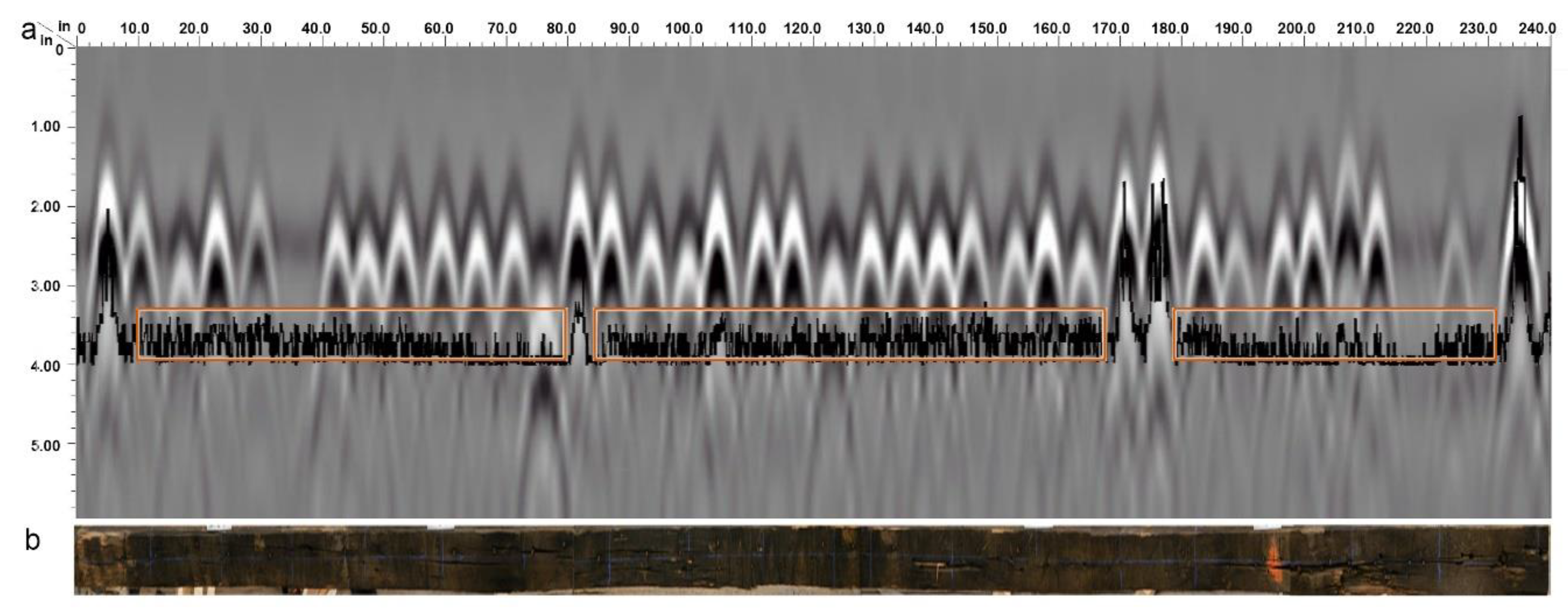
No. 10 timber has at least 60 metals, including bars and small nails in the D side. The region for the extracted reference data was successfully selected between 2540 mm and 2794 mm. Figure 13b shows the radargrams and the similarity line chart. The peak points in the orange rectangle of the line chart indicated metal. Besides these points with higher values, the other visible and highlight hyperbolae (Figure 13) were the smaller and slight points from the line chart in Figure 13. However, the blurred hyperbola (Figure 13) between 2032 mm and 2540 mm was found to be a hole after checking the images. The holes have a lower smaller similarity value than that of metal bars.
The similarity value in the red rectangle usually appeared if there are at least 2 hyperbolae. These higher value points were caused by the overlapped signal among these defects in the adjacent regions. The timbers were placed on two wood supports during testing. This experimental support produced noise in the raw data. The noise still cannot be completely removed from the reflected waves by the denoising process. The ranges of similarity values of different defects were separately recorded. The approximate locations of defects on the radargram were found by the conversion on the position of the peak from single-channel signal. A total of 737 peak points were estimated based on the similarity value. These peaks represent the metal bars, holes, knots, or other kinds of defects. All the peak points in Figure 13 were the bars or nails. The similarity values of knots were relatively small, and the fluctuation of these similarities on the line chart was slight.
Choosing the reference area from other scan lines of the same timber was also feasible when the region that has no defects was difficult to be selected in the radargrams. As shown in Figure 14, the suitable range for the basic signal was difficult to be calculated. The raw data group scanned from No. 2 scanning line, which is along the middle scanning path were evaluated for the reference data. Figure 13 shows the similarity condition using reference data that comes from another scanning path. The higher peak points in the line chart were corresponding to the hyperbolae. The higher values near the two ends were certified to be two big diameter bars. Some lower peak points inside the orange rectangle region on the line chart indicated the same type of bars. The peak points on the line chart between two neighboring rectangles indicated the metal bars. The region in the timber face for these points has at least one bar, or there are some holes and cracks around the bars. Several bars together caused the overlapped waves, which resulted in a higher similarity.
Table 4 displays the statistic results of 17 timbers. ‘NM’ means the number of metals on the surface. ‘NMP’ indicates the number of metals that could be confirmed after data processing. ‘Per’ represents the percentage of the identified defects. The highest forecast percentage is 91%, while the lowest one is about 39%. After the comparisons of all records, the following special cases may generate some errors when we evaluate the internal condition of wood timbers.
- Even though lots of the reflected waves have been shown in the radargrams as we can see, some objects inside the wood were still not successfully observed in the radargrams. When some objects were close with each other, these waves may be covered by some special wave. For these objects, the similarity could reflect the difference among them. For some objects with obscure reflected waves that could not be located as defects on the radargrams, the processing on similarity has advantages on the extraction of defects.
- Some objects shown in the radargrams sometimes were not accurately estimated according to the similarity matrix. Nearby objects influenced the values of the object. The similarity values of the overlapped wave between objects were higher than those of the objects. Or the reflected waves of one surrounding objects with a big diameter or higher dielectronic constant (DC) influenced the comparison of similarity.
- The size of the object that was not successfully shown in the radargram and failed to be located by the peak points of the similarity matrix was commonly small. For these objects, the setup of the sampling interval in the system was also one of the factors that influence the final observation. The objects probably were unsuccessfully caught by the antenna when the sampling interval was big.
- An inaccurate decision of the defects may happen due to the complex condition surround the objects, even though some objects could be detected in both radargrams and the line chart of the similarity matrix. For example, the similarity values of a small nail were similar with a big hole, and a bigger metal bar may have similar results with two closer shorter nails.
The method worked well in three cases. First, there are no same kinds of defects in the same location. Second, there are different kinds of defects in a region and the distribution between them is not particularly dense. Third, there are some defects with the same category and a different size in an area, and the distribution between them is not dense.
5. Conclusions
This study explicated the effectiveness of using GPR to locate and define the defects of wood timbers, and an object detection method based on EMD and DTW was proposed. Some bridge timbers on California Route 66 containing cracks, splits, holes, and metal bars were selected as experimental samples. We used a series of processing steps to locate the defects, including some defects that are invisible in the radargrams. EMD and DTW are efficient to process the GPR data of wood timbers. The results described the feasibility of illustrating GPR signals and extracting the defective features of radargrams using EMD and DTW. Even though EMD and DTW have shown a positive result in locating and classifying defects, there still exist some vague areas. In the future, further improvement in the proposed method for signal enhancing is necessary. The classification of the overlapping waves is also worth studying.
Author Contributions
X.W. (Xi Wu) wrote the original draft of the manuscript and performed most experiments and analysis work. G.L. and C.A.S. provided the basic idea and outline of this manuscript as well as helped revise the manuscript. J.W. and X.W. (Xiping Wang) conceived the project and provided technical guidance for this study. All authors have read and agreed to the published version of the manuscript.
Funding
This paper describes a study conducted in USDA Forest Service, Forest Products Laboratory, and it is supported partially by the National Natural Science Foundation of China (No. 61472368), 111 Project (No. B12018), Wuxi International Science and Technology Research and Development Co-operative Project (No.CZE02H1706), and the Jiangsu Agriculture Science and Technology Innovation Fund (No. CX(19)3087).
Acknowledgments
We acknowledge the technical support from staff of USDA Forest Service, Forest Products Laboratory.
Conflicts of Interest
The authors declare no conflict of interest.
References
- Pettinelli, E.; Matteo, A.D.; Mattei, E.; Crocco, L.; Soldovieri, F.; Redman, J.D.; Annan, A.P. GPR response from buried pipes: Measurement on field site and tomographic reconstructions. IEEE Trans. Geosci. Remote Sens. 2009, 47, 2639–2645. [Google Scholar] [CrossRef]
- Liu, Y.; Shi, Z.; Wang, B.; Yu, T. GPR impedance inversion for imaging and characterization of buried archaeological remains: A case study at Mudu city cite in Suzhou, China. J. Appl. Geophys. 2018, 148, 226–233. [Google Scholar] [CrossRef]
- Annan, A.P. The history of ground penetrating radar. Subsurf. Sens. Technol. Appl. 2002, 3, 303–320. [Google Scholar] [CrossRef]
- Chang, C.W.; Lin, C.H.; Yuan, Q. Quantitative study of electromagnetic wave characteristic values for mortar’s crack. Constr. Build. Mater. 2018, 175, 351–359. [Google Scholar] [CrossRef]
- Xie, F.; Wu, G.G.; Lai, W.W.; Sham, J.F. Correction of multi-frequency GPR wave velocity with distorted hyperbolic reflections from GPR surveys of underground utilities. Tunn. Undergr. Space Technol. 2018, 76, 76–91. [Google Scholar] [CrossRef]
- Schad, K.C.; Schmold, D.L.; Ross, R.J. Nondestructive methods for detecting defects in softwood logs. In Research Paper FPL-RP-546; U.S. Department of Agriculture, Forest Service, Forest Products Laboratory: Madison, WI, USA, 1996. [Google Scholar]
- Brashaw, B.K. Inspection of Timber Bridge Longitudinal Decks with Ground Penetrating Radar. Ph.D. Thesis, Mississippi State University, Starkville, MS, USA, 2014; p. 3665457. [Google Scholar]
- Shapovalov, V.; Yavna, V.; Kochur, A.; Khakiev, Z.; Sulavko, S.; Daniel, D.; Kruglikov, A. Application of GPR for determining electrophysical properties of structural layers and materials. J. Appl. Geophys. 2020, 172, 103913. [Google Scholar] [CrossRef]
- Muller, W. Timber girder inspection using ground penetrating radar. Or Insight 2003, 45, 809–812. [Google Scholar] [CrossRef]
- Maï, T.C.; Razafindratsima, S.; Sbartaï, Z.M.; Demontoux, F.; Bos, F. Non-destructive evaluation of moisture content of wood material at GPR frequency. Constr. Build. Mater. 2015, 77, 213–217. [Google Scholar] [CrossRef]
- Martínez-Sala, R.; Rodríguez-Abad, I.; Diez Barra, R.; Capuz-Lladró, R. Assessment of the dielectric anisotropy in timber using the nondestructive GPR technique. Constr. Build. Mater. 2013, 38, 903–911. [Google Scholar] [CrossRef]
- Hans, G.; Redman, D.; Leblon, B.; Nader, J.; Larocque, A. Determination of log moisture content using ground penetrating radar (GPR). Part 2. Propagation velocity (PV) method. Holzforschung 2015, 69, 1125–1132. [Google Scholar] [CrossRef]
- Razafindratsima, S.; Sbartaï, Z.M.; Demontoux, F. Permittivity measurement of wood material over a wide range of moisture content. Wood Sci. Technol. 2017, 51, 1421–1431. [Google Scholar] [CrossRef]
- Xiang, L.; Zhou, H.L.; Shu, Z.; Tan, S.H.; Liang, G.Q.; Zhu, J. Gpr evaluation of the Damaoshan highway tunnel: A case study. NDT E Inter. 2013, 59, 68–76. [Google Scholar] [CrossRef]
- Huang, N.E.; Shen, Z.; Long, S.R.; Wu, M.C.; Shih, H.H.; Zheng, Q.; Yen, N.C.; Tung, C.C.; Liu, H.H. The Empirical Mode Decomposition and the Hilbert Spectrum for Nonlinear and Non-Stationary Time Series Analysis. Proc. R. Soc. Lond. A Math. Phys. Eng. Sci. 1998, 454, 903–995. [Google Scholar] [CrossRef]
- Dragomiretskiy, K.; Zosso, D. Variational Mode Decomposition. IEEE Trans. Signal Process. 2014, 62, 531–544. [Google Scholar] [CrossRef]
- Battista, B.M.; Knapp, C.; McGee, T.; Goebel, V. Application of the empirical mode decomposition and Hilbert–Huang transform to seismic reflection data. Geophysics 2007, 72, 29–37. [Google Scholar] [CrossRef] [Green Version]
- Narayanan, R.M.; Shastry, M.C.; Chen, P.-H.; Levi, M. Through -the-Wall Detection of Stationary Human Targets Using Doppler Radar. Prog. Electromagn. Res. B 2010, 20, 147–166. [Google Scholar] [CrossRef] [Green Version]
- Mallat, S. A Wavelet Tour of Signal Processing: The Sparse Way; Academic Press: Burlington, MA, USA, 2008; pp. 98–99. [Google Scholar]
- Bekara, M.; Baan, M.V.D. Random and coherent noise attenuation by empirical mode decomposition. Geophysics 2009, 74, 89–98. [Google Scholar] [CrossRef]
- Zhu, B.Z.; Yuan, L.L.; Ye, S.X. Examining the multi-timescales of European carbon market with grey relational analysis and empirical mode decomposition. Phys. A Stat. Mech. Appl. 2019, 517, 392–399. [Google Scholar] [CrossRef]
- Jazayeri, S.; Saghafi, A.; Esmaeili, S.; Tsokos, C. Automatic Object Detection using Dynamic Time Warping on Ground Penetrating Radar Signals. Expert Syst. Appl. 2019, 122, 102–107. [Google Scholar] [CrossRef]
- Ratanamahatana, C.A.; Keogh, E. Everything you know about dynamic time warping is wrong. In Proceedings of the Third Workshop on Mining Temporal and Sequential Data, in Conjunction with 10th ACM SIGKDD International Conference on Knowledge Discovery and Data Mining (KDD-2004), Seattle, WA, USA, 22–25 August 2004; pp. 22–25. [Google Scholar]
- Zhen, D.; Wang, T.; Gu, F.; Ball, A.D. Fault diagnosis of motor drives using stator current signal analysis based on dynamic time warping. Mech. Syst. Signal Process. 2013, 34, 191–202. [Google Scholar] [CrossRef] [Green Version]
- Parziale, A.; Diaz, M.; Ferrer, M.A.; Marcelli, A. SM-DTW: Stability Modulated Dynamic Time Warping for signature verification. Pattern Recognit. Lett. 2019, 121, 113–122. [Google Scholar] [CrossRef]
- Jain, B.J. Making the dynamic time warping distance warping-invariant. Pattern Recognit. 2019, 94, 35–52. [Google Scholar] [CrossRef] [Green Version]
- Tosti, F.; Ciampoli, L.B.; Calvi, A.; Alani, A.M.; Benedetto, A. An investigation into the railway ballast dielectric properties using different GPR antennas and frequency systems. NDT E Inter. 2018, 93, 131–140. [Google Scholar] [CrossRef]
- Benson, A.K. Applications of ground penetrating radar in assessing some geological hazards: Examples of groundwater contamination, faults, cavities. J. Appl. Geophys. 1995, 33, 177–193. [Google Scholar] [CrossRef]
- Wacker, J.; Mikhail, M.; Dizon, G. Evaluation of Bridge Components Salvaged from Historic Route 66 in California; Research in Progress RIP-4719-038; USDA Forest Service, Forest Products Laboratory: Madison, WI, USA, 2017; Available online: https://www.fpl.fs.fed.us/documnts/rips/fplrip-4719-038-Wacker-Mikhail-Dizon.pdf (accessed on 4 February 2020).
- Li, H.; Qin, X.; Zhao, D.; Chen, J.; Wang, P. An improved empirical mode decomposition method based on the cubic trigonometric b-spline interpolation algorithm. Appl. Math. Comput. 2018, 332, 406–419. [Google Scholar] [CrossRef]
Figure 1.
The setting of an antenna position and a target position.
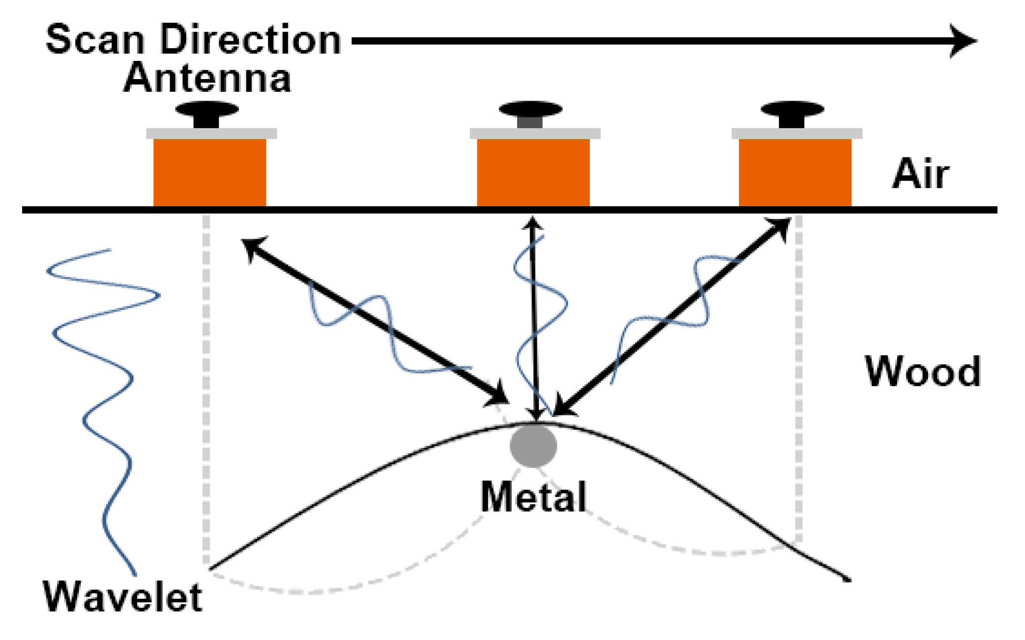
Figure 2.
The three-dimensional model of the timbers. A and F are the left and right sides, E and C represent the bottom and top sides with 381 mm width, B and D denote the front and back sides with 101.6 mm thickness.
Figure 2.
The three-dimensional model of the timbers. A and F are the left and right sides, E and C represent the bottom and top sides with 381 mm width, B and D denote the front and back sides with 101.6 mm thickness.
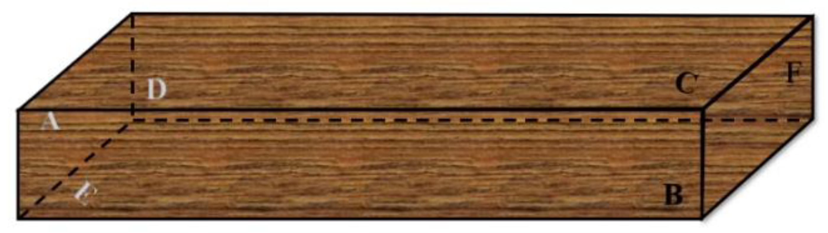
Figure 3.
The ground-penetrating radar (GPR) scan lines of the timbers. (a)The middle scan line on B or D side; (b)Three scan lines on C or E side.
Figure 3.
The ground-penetrating radar (GPR) scan lines of the timbers. (a)The middle scan line on B or D side; (b)Three scan lines on C or E side.
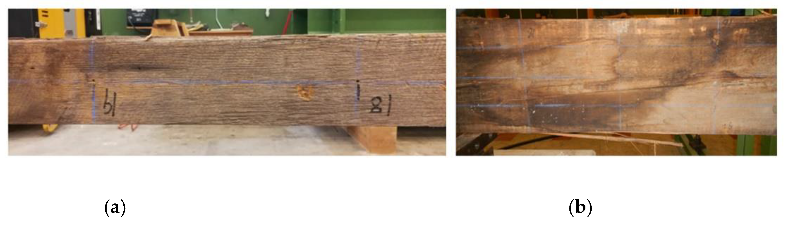
Figure 4.
Defect accounts for 18 timbers.
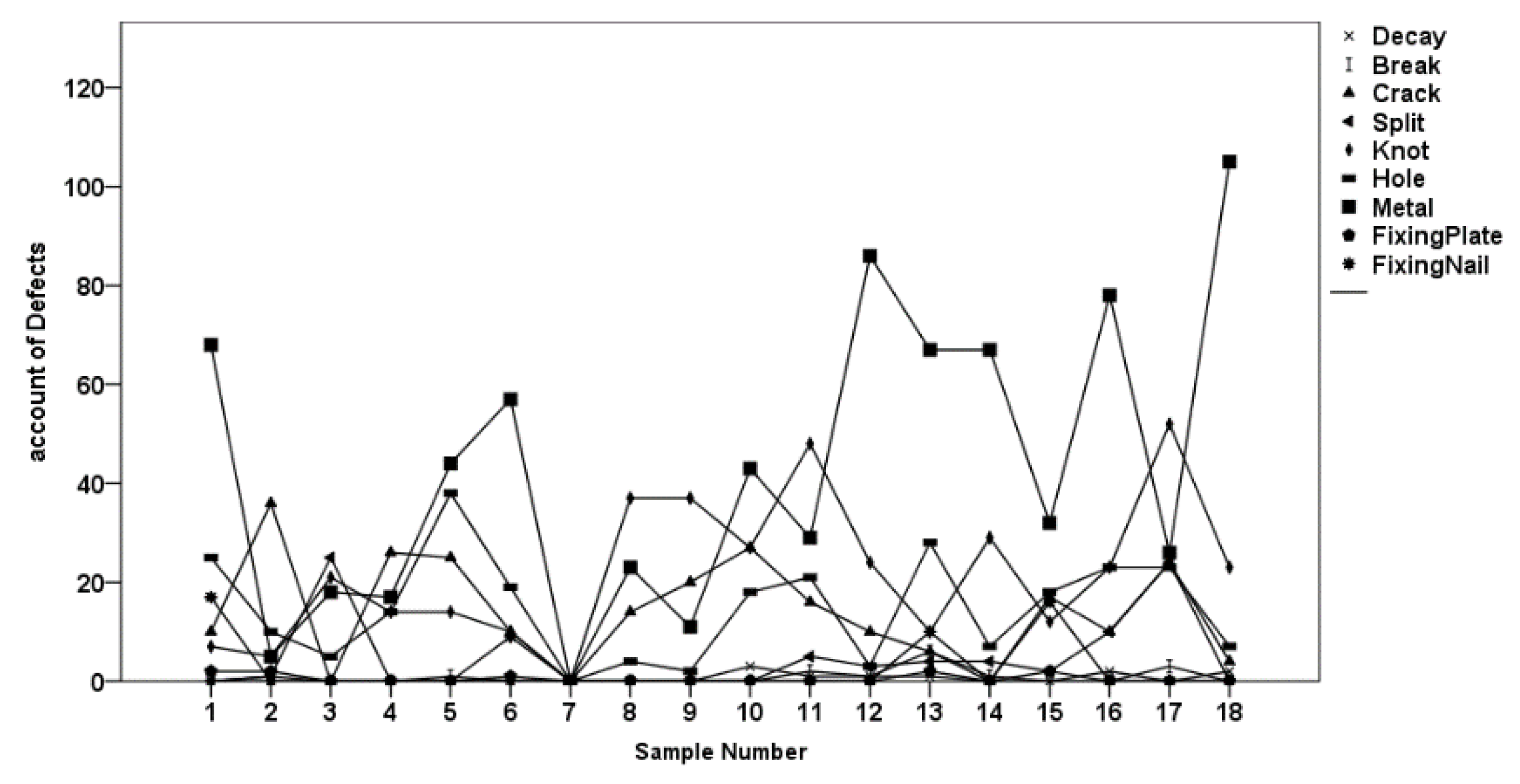
Figure 5.
The testing environment of core-samples. (a) The core-samples inserted with metals; (b) The timber-section with core-samples.
Figure 5.
The testing environment of core-samples. (a) The core-samples inserted with metals; (b) The timber-section with core-samples.
Figure 6.
The results of one signal after empirical mode decomposition (EMD) analysis. (a) The Intrinsic Mode Function (IMF) components; (b) The frequency spectrum.
Figure 6.
The results of one signal after empirical mode decomposition (EMD) analysis. (a) The Intrinsic Mode Function (IMF) components; (b) The frequency spectrum.
Figure 7.
The squared Euclidian distance matrix between two time series signals.

Figure 8.
The comparison of the similarity values and the B-scan image of No. 6 core-sample. (a) The similarity values of core-samples with different moisture content (MC); (b) The radargrams of timber sections inserted with No. 6 core-sample.
Figure 8.
The comparison of the similarity values and the B-scan image of No. 6 core-sample. (a) The similarity values of core-samples with different moisture content (MC); (b) The radargrams of timber sections inserted with No. 6 core-sample.
Figure 9.
GPR scanning after inserting core-samples into the timber section.

Figure 10.
The comparison of the similarity value and the B-scan image of core-sample inserted with metal bar. (a) The similarity value of one core-sample inserted with metal bar; (b) The B-scan image of the core-sample.
Figure 10.
The comparison of the similarity value and the B-scan image of core-sample inserted with metal bar. (a) The similarity value of one core-sample inserted with metal bar; (b) The B-scan image of the core-sample.
Figure 11.
One B-Scan image of No. 11 timber.

Figure 12.
One B-Scan image of No. 6 timber.
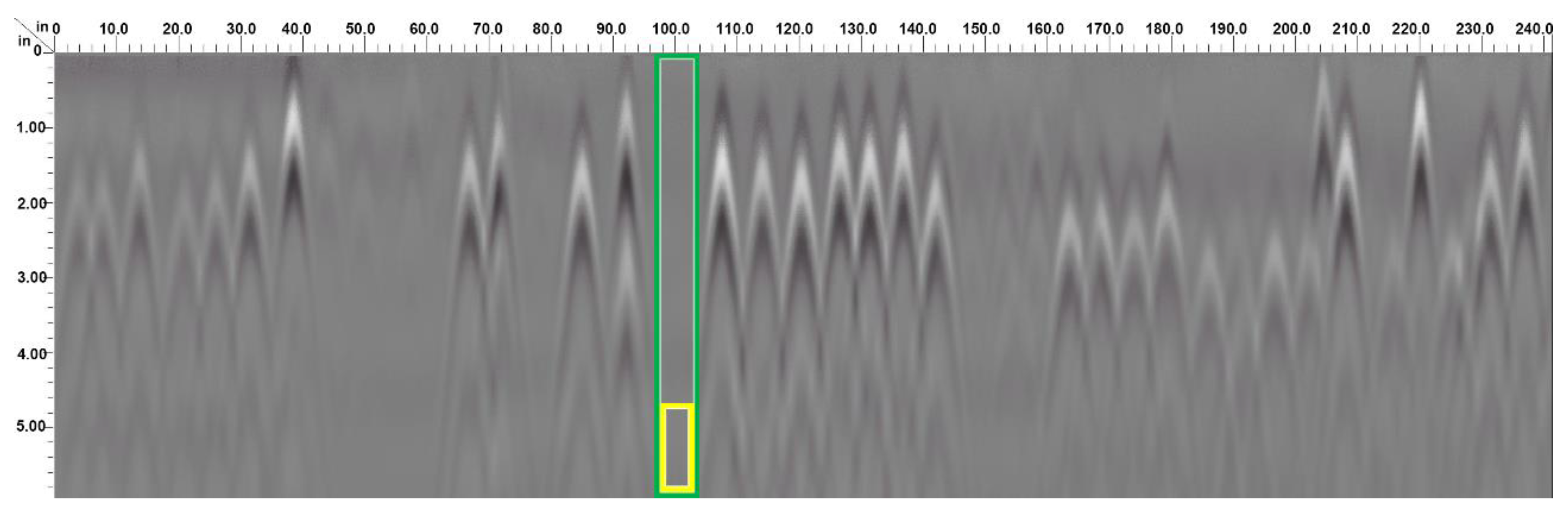
Figure 13.
The combined image for the line chart of dynamic time warping (DTW) value, the radargrams generated from RADAN 7, and the outside camera pictures (sample NO. 10). (a) The results made up of the radargrams and the line chart of similarity; (b) The outside image of one side of No. 10 timber.

Figure 14.
The combined image for the line chart of DTW value, the radargrams generated from RADAN 7, and the outside camera pictures (sample No. 13). (a) The results made up of the radargrams and the line chart of similarity; (b) The outside image of one side of No. 13 timber.
Figure 14.
The combined image for the line chart of DTW value, the radargrams generated from RADAN 7, and the outside camera pictures (sample No. 13). (a) The results made up of the radargrams and the line chart of similarity; (b) The outside image of one side of No. 13 timber.

Table 1.
The characteristics of 7 core-samples.
| NO. | Diameter (mm) | Length (mm) | Volume (m3) |
|---|---|---|---|
| 1 | 68.263 | 133.350 | 4.880 × 10⁻⁴ |
| 2 | 66.675 | 133.350 | 4.880 × 10⁻⁴ |
| 3 | 68.263 | 133.350 | 4.880 × 10⁻⁴ |
| 4 | 68.263 | 133.350 | 4.880 × 10⁻⁴ |
| 5 | 68.263 | 133.350 | 4.880×10⁻⁴ |
| 6 | 68.263 | 133.350 | 4.880 × 10⁻⁴ |
| 7 | 68.263 | 133.350 | 4.880 × 10⁻⁴ |
Table 2.
Moisture content of the soaked core-samples.
| NO. | Moisture Content (%) | |||||
|---|---|---|---|---|---|---|
| 0 h | 2 h | 7.5 h | 24 h | 55.5 h | 120 h | |
| 1 | 6 | 14 | 20 | 27 | 35 | 46 |
| 2 | 6 | 14 | 19 | 23 | 36 | 47 |
| 3 | 6 | 15 | 21 | 28 | 35 | 45 |
| 4 | 6 | 14 | 18 | 25 | 31 | 39 |
| 5 | 6 | 14 | 19 | 26 | 33 | 42 |
Table 3.
Control Parameter settings used on Subsurface Interface Radar (SIR)-4000 unit.
| Radar-Parameter | Setting/Value | Process-Parameter | Setting/Value |
|---|---|---|---|
| Collect Model | Distance Mode | Gain Model | Manual |
| Scans/Second | 200 | Edit Gain Curve | 8 Points |
| Samples/Scan | 512 | FIR (Finite Impulse Response) Low Pass | 4000 MHz |
| Scans/In | 10.0 | FIR High Pass | 500 MHz |
| In/Mark | 120.0 | FIR Stacking | Off |
| Soil Type | Custom | FIR BG Removal | 0 |
| Time Range | 3.00 (ns) | IIR (Infinite Impulse Response) Low Pass | Off |
| Position Model | Manual | IIR High Pass | 10 MHz |
| Offset | 11.90 | IIR Stacking | 0 |
| Surface | 0 (%) | IIR BG (Background) Removal | 0 |
| Signal Floor | Off | ||
| Filters | Off |
Table 4.
The statistics of defects based on the defects mapping and peaks of the similarity value.
| NO. | 1 | 2 | 3 | 4 | 5 | 6 | 8 | 9 | 10 | 11 | 12 | 13 | 14 | 15 | 16 | 17 | 18 |
|---|---|---|---|---|---|---|---|---|---|---|---|---|---|---|---|---|---|
| NM | 60 | 5 | 14 | 7 | 41 | 55 | 22 | 9 | 63 | 23 | 77 | 64 | 61 | 37 | 72 | 24 | 94 |
| NMP | 39 | 3 | 8 | 4 | 24 | 42 | 20 | 7 | 45 | 21 | 36 | 33 | 24 | 28 | 36 | 17 | 50 |
| Per (%) | 65 | 60 | 57 | 57 | 59 | 76 | 91 | 78 | 71 | 91 | 47 | 52 | 39 | 76 | 50 | 71 | 53 |
© 2020 by the authors. Licensee MDPI, Basel, Switzerland. This article is an open access article distributed under the terms and conditions of the Creative Commons Attribution (CC BY) license (http://creativecommons.org/licenses/by/4.0/).
Share and Cite
MDPI and ACS Style
Wu, X.; Senalik, C.A.; Wacker, J.; Wang, X.; Li, G. Object Detection of Ground-Penetrating Radar Signals Using Empirical Mode Decomposition and Dynamic Time Warping. Forests 2020, 11, 230. https://doi.org/10.3390/f11020230
AMA Style
Wu X, Senalik CA, Wacker J, Wang X, Li G. Object Detection of Ground-Penetrating Radar Signals Using Empirical Mode Decomposition and Dynamic Time Warping. Forests. 2020; 11(2):230. https://doi.org/10.3390/f11020230
Chicago/Turabian StyleWu, Xi, Christopher Adam Senalik, James Wacker, Xiping Wang, and Guanghui Li. 2020. "Object Detection of Ground-Penetrating Radar Signals Using Empirical Mode Decomposition and Dynamic Time Warping" Forests 11, no. 2: 230. https://doi.org/10.3390/f11020230
Note that from the first issue of 2016, this journal uses article numbers instead of page numbers. See further details here.