US National Maps Attributing Forest Change: 1986–2010
by

Karen G. Schleeweis
1,*, 
Gretchen G. Moisen
1, 
Todd A. Schroeder
2,
Chris Toney
1,
Elizabeth A. Freeman
1,
Samuel N. Goward
3,
Chengquan Huang
3 and
Jennifer L. Dungan
4 1
Forest Inventory and Analysis, U.S. Forest Service, Rocky Mountain Research Station, 507 25th Street, Ogden, UT 84401, USA
2
Forest Inventory and Analysis, U.S. Forest Service, Southern Research Station, 4700 Old Kingston Pike, Knoxville, TN 37919, USA
3
Department of Geographical Sciences, University of Maryland, 2181 Samuel J. LeFrak Hall, College Park, MD 20742, USA
4
NASA Ames Research Center, Moffett Field, CA 94035, USA
*
Author to whom correspondence should be addressed.
Forests 2020, 11(6), 653; https://doi.org/10.3390/f11060653
Submission received: 13 November 2019
/
Revised: 19 May 2020
/
Accepted: 28 May 2020
/
Published: 8 June 2020
(This article belongs to the Special Issue Estimating change in forests: Merging Ground-, Photo-, and Space-Based Observations)
Abstract
:National monitoring of forestlands and the processes causing canopy cover loss, be they abrupt or gradual, partial or stand clearing, temporary (disturbance) or persisting (deforestation), are necessary at fine scales to inform management, science and policy. This study utilizes the Landsat archive and an ensemble of disturbance algorithms to produce maps attributing event type and timing to >258 million ha of contiguous Unites States forested ecosystems (1986–2010). Nationally, 75.95 million forest ha (759,531 km2) experienced change, with 80.6% attributed to removals, 12.4% to wildfire, 4.7% to stress and 2.2% to conversion. Between regions, the relative amounts and rates of removals, wildfire, stress and conversion varied substantially. The removal class had 82.3% (0.01 S.E.) user’s and 72.2% (0.02 S.E.) producer’s accuracy. A survey of available national attribution datasets, from the data user’s perspective, of scale, relevant processes and ecological depth suggests knowledge gaps remain.
Keywords:
forest cover loss; disturbance; conversion; attribution; Landsat time series; Random Forests; NAFD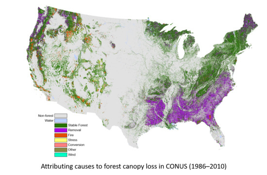
1. Introduction
Change is fundamental to current and future forest functions. Events that reduce cover differentially affect forest spatial configurations [1], recovery rates and succession [2,3,4,5,6,7,8,9,10], can have complex interactions through time [11,12,13,14,15,16], and affect ecosystem functions and resilience [17,18,19,20,21,22,23]. Data on the specific event type (as well as magnitude, spatial and temporal characteristics) are necessary for descriptive, predictive and prescriptive analytics [24,25,26,27] for understanding feedbacks between forest dynamics, climate, ownership, policy and markets [28,29,30,31,32,33,34,35,36,37,38,39,40].
Datasets produced to inform scientists, land managers and policy makers about forest status and trends have progressed over time with technology and user needs. Historically, statistical inventories, such as the U.S. Department of Agriculture’s Forest Service’s (USFS) Forest Inventory Analysis (FIA) and the National Resource Conservation Service’s (NRCS) National Resource Inventory (NRI), provided the nation’s forest monitoring and land use change data, respectively [41,42]. These inventory programs, once decadal, have responded to needs for statistically sound estimations derived from more frequent sample periods [43,44]. The USFS and NRCS have always used high-resolution aerial imagery to view plot locations at the time of ground-based sampling, to help reduce costs and improve efficiencies.
A proliferation of national- and continental-scale, satellite-based forest maps have become available, due to the legacy of moderate resolution imagery from spaceborne sensors such as Landsat, free public access to the Landsat archive, and the availability of high-end computing capabilities [45,46,47]. Some mapping approaches are more manually intensive, balancing expert knowledge with automatic algorithms and expending large efforts on final cartographic cleanliness [48,49], while others put a high premiums on full automation [50,51]. Some national maps of forest change are produced from single collections (a collection of imagery from a sensor processed with a single method through time) using multi-year time steps (4+ years between sequential image observations) [52,53], single collections for annual (or higher step) time series stack analysis [54,55], and multiple collections for multi-year time steps [49,56,57]. In addition, each change detection algorithm has its own merits and limitations [58,59,60]. In dense time series image stacks, abrupt changes in forest cover are aptly found by change algorithms focused on statistical anomalies [61,62], while slower and more subtle changes are more readily captured by segment- or trajectories-based algorithms [63,64]. Algorithms based on fitting curves to the time series signal and analyzing the residuals can capture subtler, faster changes between and within seasons [65,66,67,68]. The capturing of a change and the attribution of a causal process are often achieved at different steps in the workflow or processing stream.
This paper focuses on research into the attribution of event types to forest canopy cover loss events in the contiguous US. We introduce a new spatial dataset, the North American Forest Dynamics-Attribution (NAFD-ATT) data, which attributes the most common event types (no event, removal, fire, stress, conversion and wind) to forests in the conterminous U.S. (CONUS) between 1986 and 2010. A goal of this study was to employ the outputs from multiple forest change algorithms to differentiate all major types of fast (removals, fire, wind and conversion) and slow (stress) disturbances, and to differentiate between temporary (disturbance) and persistent canopy loss (deforestation) processes. The North American Forest Dynamics (NAFD) project was a long-term collaboration between the University of Maryland, NASA and the U.S. Forest Service, Forest Inventory and Analysis (USFS FIA) program [54,69,70]. The primary NAFD goal was to increase the spatial and temporal accuracy of national-scale assessments of forest disturbance dynamics, for carbon cycle science under NASA’s North American Carbon Program.
Table 1 lists available CONUS attribution datasets, highlighting salient differences between the products from a user’s perspective of scale, processes and metrics of ecological significance. It is known that areal measures derived from estimation and mapping do not always coincide [71]. Table 1 highlights estimated products (light grey), mapped products (dark grey) and hybrid products (medium grey). To evaluate which dataset might be more appropriate for their needs, based on possible reporting and analysis scales, users can look under the temporal and spatial row tabs in Table 1. Referencing this table, data users can easily look to see if a data product captures within-class changes, such as degradation or partial forest removals, or a particular process of interest. Monitoring Trends in Burn Severity (MTBS) attributes and maps only one process: annual fire events on all lands [72]. A testament to its efficacy in mapping this one process, MTBS data is ingested by most of the other projects that attribute fire, including NAFD-ATT [50,53,73,74]. Other users may want to focus on ecologically relevant metrics to monitor and describe disturbance regimes, such as frequency, succession, magnitude and duration [75,76].
The NAFD-ATT map and data products were created from statistically sampled training data, across all ownerships of forested land, and a nationally consistent machine learning approach across the CONUS, yielding 25 years of forest event type history. These products will be available from the Oak Ridge National Laboratory (ORNL) Distributed Active Archive Center (DAAC) (Available on-line (http://daac.ornl.gov) from ORNL DAAC, Oak Ridge, Tennessee, USA. https://doi.org/10.3334/ORNLDAAC/1799) and the USFS geospatial data platform. According to the results presented here, between 1986 and 2010, 70.6% of all CONUS forests remained stable without loss events. Temporary canopy loss from removals, fire and stress were attributed to the majority of canopy loss events (70.7%, 23.6%, 3.6%, and 1.4% of all forest land respectively) and only 0.6% of all forest land had canopy loss events attributed to land use/cover change (persisting forest loss). Further spatio-temporal results, accuracy measures, limitations and next steps are reported in the manuscript.
2. Materials and Methods
2.1. Training Data
We used a sample of 7200 plots across the CONUS, collected using TimeSync software for the North American Forest Dynamics (NAFD) project as the response data for the classification model [77]. A stratified two-stage sample design was used to collect the plots. The five strata used are coarse generalizations combining different ecoregions that share similar forest types. Selecting more samples in strata with more abundant and diverse forest increased the likelihood that response plots would fall on forestland and, by extension, that more forest change would be captured. Theissen polygons, calculated using the center points of the Landsat World Reference System path-row grid, comprised the non-overlapping sample units. Of the 442 Theissen polygon sample units that overlap CONUS boundaries, 180 were randomly selected from within the five strata. Within each sample unit, 40 plots were randomly distributed. A total of 2700 of the training plots fell on land that had forest cover (planted or naturally vegetated land likely to contain 10% or greater tree cover at some time during the time series sequence). Full details of the sample and response design of the training dataset and related visuals are published [73].
The plot observations were collected on each plot (30 × 30 pixel) using annual cloud-filled Landsat time series stacks (nominally from 1984 to 2012) within TimeSync software, ancillary datasets and high resolution aerial imagery in Google Earth where available [54]. Analysts temporally segment the data (image series) by labeling and recording visual observations of land cover, land use and change processes at the plot level [77]. Plots originally labeled “Mechanical” change processes and which occurred in forest cover were relabeled to “removals” or “conversion,” depending on the land cover/use and timing observations in the plot records. At the end of the imagery time series, it is harder to determine with confidence whether a forest clearing activity was related to conversion or removals. We cautiously labeled all mechanical clearings as removals, if they occurred within six years of the end of the time-series stack, unless evidence of specific land use change was recorded.
In addition to these plots, further training data, gathered for the pilot study, included plots from the LANDFIRE project, FIA ground data and analyst interpretation of Landsat/aerial time-series images using TimeSync software [78]. These additional, opportunistically gathered data, not appropriate for inference, were not used in calculating (OOB) accuracy measures [79].
2.2. Predictor Variables
Forest disturbance algorithms have unique sets of costs and benefits in terms of errors omitted (false negatives) and committed (false positives) for each forest disturbance event type [58]. We used outputs from three change algorithms as predictor variables to mitigate omissions. The vegetation change tracker (VCT) algorithm excels with abrupt disturbance processes of varying magnitude [61,80]. The Shapes algorithm is a spline approach constrained by a priori defined spectral trajectory “behaviors”, based on forest ecology principles, including long slow declines [81,82,83]. MTBS burn severity raster data reflect known fire events that meet a certain minimum size criterion [84]. The Shapes and VCT algorithms were run on NAFD Landsat time-series stacks including nominal imagery from 1984 to 2011. We subset all algorithm outputs to the years 1986–2010.
As part of the North American Forest Dynamics (NAFD) project, access to NASA’s high end computing capability (HECC) and the NASA Earth Exchange (NEX) collaborative platform allowed for efficient national scale data prep, storage and processing on 25 years of Landsat data [85]. Over 60,000 Landsat images from the 1984–2011 time period (Landsats 4–7 Thematic Mapper) were evaluated for processing and analysis as part of the NAFD processing stream. Landsat image processing, completed using various Landsat Ecosystem Disturbance Adaptive Processing System (LEDAPS) and VCT modules, included conversion to surface reflectance, atmospheric adjustment, individual scene masking (for clouds, shadow, snow, bad data and water), intra-annual growing season clear view compositing, vegetation index calculation, assembling and clipping individual year images into a time-series stack, and between-year data interpolation (in areas of no observations). After clear view compositing, 62% of the annual images in the time-series were clear-view, 27% were clear composites, 9% had remaining cloud contamination and 2% had no acceptable images. Full descriptions of image selection, quality and the image processing streams are available in previous publications [54,86].
We ran Shapes on the Landsat time-series stacks (see above) of Normalized Difference Vegetation Index (NDVI), band 5 surface reflectance, Forestness Index (FI) and Normalized Burn Ratio (NBR), yielding band specific temporal, magnitude and classified “shape” metrics for each band.
Annual VCT rasters, generated as part of the NAFD project and referred to here as NAFD-NEX maps, included annual maps of the year of disturbance onset and multiple magnitude indices. We converted VCT disturbance year rasters to annual polygon records and their calculated area, perimeter, shape and fractal indices. Using a “most recent” event per pixel rule, the annual polygon data and related metrics were composited into single date, geometry and magnitude layers. The same rule was applied to the annual magnitude rasters to create a composite layer for each metric.
Annual MTBS burn severity raster data were composited into a presence/absence layer using the low, moderate and high intensity values. In the case of more than one fire event in a pixel through time, the highest magnitude event date (year) was selected. The most recent event was selected in cases where multiple highest magnitude events occurred in the same location. Selected pixels were composited into a binary fire layer and a separate corresponding year of fire layer.
Local geographic predictors included aspect, slope, latitude and longitude, elevation and transformed aspect. Vegetation predictors include USFS forest group type and probability, down sampled from 250 to 30 m [87], and LANDFIRE Existing Vegetation Type (EVT v1.4.0) data collapsed to three classes: agriculture, forest and developed [88].
2.3. Modeling Process
A pilot study of 10 Landsat scene locations demonstrated that a two-step “flat-to-annual” process reliably separates multiple classes of canopy change activities [78]. In the first step, we construct a categorical Random Forest [79] for event type response classes using the R ModelMap package [89]. In the second step, disturbance year (and duration in the case of the stress category) were calculated using a rule-based approach and temporal metrics from the three predictor disturbance algorithms (see Section 2.2).
Modeling continuously across the nation brings different methodological and validation challenges from modeling in localized regions [90]. We tested building and predicting models over different geographic combinations of training data strata, aggregating response classes and down sampling to mitigate imbalanced training data. We visually compared predicted maps from model runs to published geospatial data sets on different process types to select the most representative model predictions. To provide insight into variable importance, we compared per class commission and omission from models constructed with different suites of training data.
2.4. Accuracy Assessment
We followed the best practices for robustly estimating map accuracy from Olofsson et al. [91] where possible. Reference data for multiple disturbance types is difficult to attain, so we used all training data to build the model, rather than hold out for validation. We used the R survey package [92,93] to calculate OOB errors for the stratified two-stage design for the five reference data strata. This yielded estimates of overall accuracy, user’s accuracy (for commission errors) and producer’s accuracy (for omission error) statistics, each with associated sampling variance, standard errors and confidence intervals for each response class. The analysis conducted was consistent with the sampling and response design of the training data. For additional information on the map quality, we created two confidence layers reflecting qualitative measures of model confidence and dominance. Random Forest creates a vector of values with proportions of votes from the forest of trees for each of the response classes and selects the class with the majority proportion of votes as the winning prediction class for each prediction unit (pixel). To document the strength or confidence of the model call, we subtracted the second highest vote proportion from the highest proportion (from the winning response class) [94]. The highest possible score is 100, representing the largest possible separation between the winning and the next common class, and therefore more model “confidence.” We calculated Simpson’s dominance index [95] by summing the squares of the vote proportions for each response class on each prediction unit (pixel). This dominance index provides a measure of the dominance of the winning class. Values closer to 100 reflect a higher dominance (of one class over the others). A decreased or lower dominance would be related to a related rise in the equitable distribution of the class proportions, especially if the number of classes with votes increases; while this type of diversity is desirable in natural systems, in our categorical map predictions it is not.
3. Results and Discussion
3.1. CONUS Map of Event Type
The spatial patterns of the most dominant types of canopy cover loss events are visible when mapped (Figure 1). Stable forest—forests with no loss event between 1986 and 2010—is the largest class. Though stable from a loss perspective, these forests may be in phases of regrowth, recovery or reforestation. Removals occurred in 612,200 km2 (23.6%) of CONUS forests, with regional centers of large commercial forestry activity apparent even in national scale maps. Nearly 41% of the southern forest area had removal events over the 25-year period. Large clusters of fire activity are distinct even at this small scale (1:26,000,000), mostly in the West, with a few large fires visible along the eastern seaboard. Fire occurred in 94,483 km2 (3.6%) of CONUS forests.
The training data defined stress as any event resulting in slow gradual loss of forest canopy, including insect damage, drought and disease, which often co-occur. Most of the 35,563 km2 (1.4%) of CONUS forests affected by stress events were in the Rocky Mountain (RM) FIA region. Note, this area is calculated with onset-based (extensification) accounting, where an event is counted once at the year of onset/detection, rather than with duration (intensification), where an event is counted again in each year of the decline. Stress usually affects a narrow subset of tree species in the forested landscape, leaving a dispersed spatial patter that is difficult to visualize on a national map. The relatively rare (across regional to national landscapes) footprints of conversion and wind events are also hard to view on a map of this scale. The forestland area affected by each of these event types is 16,655 km2/year and 166 km2/year, respectively.
3.2. Annual Rates by Event Type
Annually, the prominence of a change type can vary widely within and between regions, though the inter-region dominance of each change class by region is mostly stable (Figure 2). For example, removals occur most in southern forests through the period of observation, though the annual rate of southern removals fluctuates a good deal. The magnitude, direction and variability of the southern removal rate (area/year) drives trends in the national removal rate, and makes up more than half of the total national forest canopy loss rate in most years. The multi-year trends in the southern rate are echoed in the national removal rate. Noticeable are the peaks of activity in 1989, 1998 and 2006, the latter followed by a precipitous decline likely due to the economic recession of the late 2000s. By the end of the record (2010), the removal rates returned to almost 1986 levels. Northern forests contribute the second highest area per year to national numbers, rising in 1998 to the steady rate that remained through 2010.
Annual removal rates reported here are lower than FIA decadal harvest estimates. FIA estimates report consistent harvest rates of 45,000 km2/year (3500 km2 is in interior Alaska), with variability in the proportions of “clear cut” and “partial harvest” events by region through time [96,97]. Tao et al. [98] used NAFD and FIA plot data to map the percentage of basal area removed, and found that the fluctuations in overall rates were driven primarily by variability in the rates of partial (<80% basal area) removal events, while rates for clearing events (>80% of basal area) were stable over the 25-year record. Harvest intensity and management objectives, i.e., commercial versus sanitation harvest, are critical information for evaluating the relationship between harvest rates and social, economic and environmental drivers [70,99,100]. Likewise, information on the type and method of cut, which can help determine potential product lines, decay rates and residue ratios, is important for carbon cycling, but difficult to know from remote sensing data alone [101,102]. In areas with large commercial operations and/or quick stand rotations, where stands often undergo more than one treatment before the “final cut” or clearing, our approach may underestimate annual removal areas. For example, annual NAFD-NEX maps record that 15.3% of disturbed forest locations had two distinct canopy loss events in the 25-year record, and another 1.3% had more than two [80].
The National Interagency Coordination Center reports steep spikes in national wildfire acreage in 1988, 1990, 1994, 1996, 1999, 2000, 2002 and 2004–2007 [103], similar to the peak forest fire years in these data (Figure 2). Interior West forests have the highest variability in annual forest fire area, with multiple increases in successive years (i.e., 2004–2007). As expected for event types driven by large climatic patterns, forest fire rates in the neighboring Rocky Mountain (RM) and Pacific Coast (PAC) forests have similar fire ecology and peak fire years. Southern forest fire rates have different peak years than the peak years for western forest fires, suggesting different regional climatic drivers than in the West. The similarly timed crests in the overall national rates of canopy loss are evidence of the large areas affected in peak western forest fire years.
Counting locations with repeat fires (using low, medium and high severity pixels) from MTBS, we found 10.1% of locations had two fire events and 2.27% had more than two fire events (1986–2010). These MTBS estimates are for all lands, and so will be higher than for forest fire events only. Still, the composite approach used in this study, which only records one event through time, is likely to underestimate sequentially occurring canopy loss events.
Studies suggests that large tracts of forest have been in a state of declining health for decades [73,104,105,106]. The annual rates for stress record a large spike at the beginning of the record, which is orders of magnitude larger than the mostly consistent rates in other years, and is almost all attributed to RM forests (Figure 2). It is plausible that, in this study, the spike in observations of events characterized by long slow declines in canopy cover are correctly attributed. Most time-series analyses discount or discard the first and last year of analysis due to confusion between signal and noise in the first and last year of the time-series, due to spurious clouds or the weaker quality control measures, that often make change detection more difficult and increase false positives [94,107,108,109]. This study likewise discarded the first and last year of the analyses to limit spurious false positives. The image stacks included nominal imagery between 1984 and 2011, but the analyses only report changes detected between 1986 and 2010. Further, the slow long duration decline “shape” in the Shapes algorithm, which is mostly associated with the stress class, cannot be “triggered” by a year or two of erroneous data, even at the beginning of the record of observation. The decline “shape” requires an accumulation of multiple years in the spectral signature [83]. Decline events that began before the period of observation in 1984—for example, an insect infestation or severe drought that began in 1980, and continued or intensified through the beginning of the time-series of observations—are simply attributed the first year label available, which in this case is 1986. It is important to note that 1986 may not be the peak year of the decline. Still, the challenges of correct temporal attribution (year of onset) are separate from the plausibility that the event is correctly attributed as decline and accurately reflects a steady slow decline in the spectral response of the forest canopy. The temporal requirements of the decline “shape” in the algorithm make true change less detectible (perhaps yielding more false negatives) at the end of the temporal record. In the case of slow decline events, problems of false negatives at the end of the time-series are a reality for all change detection algorithms. Training data for the stress class did not include abrupt insect mortality events, such as the widespread mortality from Southern Pine Beetle, so this class cannot be used for investigations into outbreaks of this endemic pest [110].
Accounting methods (see Section 3.1) for long duration canopy loss processes can produce widely different interpretations. This study mapped peak annual rates for the stress class of 0.3% of CONUS forest area. Cohen et al. [73] estimate two values for peak annual stress rates in 2001, depending on whether intensification or extensification accounting was used. When only one observation on the same plot was counted, regardless of the number of sequential years of decline, they estimated a peak rate of decline in 2011 of less than 0.5% of all CONUS forest area affected. When observations on the same plot were counted in each sequential year that the decline persisted, they estimated that the peak rate of decline (2011) occurred on roughly 3.0% of all CONUS forest area. Though rates between these two studies are similar if the same temporal metric is used (0.3% of CONUS forest land vs. 0.5% of CONUS forest land), comparisons are confounded by differences in area of detected stress (numerator) and/or total forest area (denominator), which are difficult to tease apart when reported as ratios (percent of total forest area). Furthermore, the studies use different methods for calculating onset year and/or duration, and different regional reporting boundaries. This study used regional boundaries defined by FIA regions. Cohen et al. used regional reporting boundaries defined by their custom strata (see Section 2.1). Other studies offer mixed reporting methods for insect-related canopy loss through time, with the majority using onset accounting [111,112,113,114,115,116].
Rates of forestland conversion first show an increase from the beginning of the time-series to a peak in 1998, at 1073 km2/year (0.04% of CONUS forest/year), then a steady and steep annual decline to 250 km2 in 2010—half of the 1986 rate (Figure 2). The timing and direction of these trends agree with the findings of both the attribution pilot study [117] and the NRI estimates, the latter inventory pertaining to mostly rural, non-Federal lands [118]. The NRI shows a peak rate in newly developed lands from forest lands of 3804 ± 76 km2/year (1992–1997 inventory), then a sharp decline to a rate of 1133 ± 38 km2/year (2007–2012 inventory), a little less than half of its estimated 1982–1987 annual rate.
Land use conversion and wind activities affect relatively small percentages of forest area at the national level, but locally are important drivers of persistent and temporary forest change, particularly in southern forests [4,31,119,120,121,122,123,124]. Gathering training data on rare classes across large landscapes is difficult with statistical sampling designs, as is using/validating imbalanced data in statistical multi-class models [125,126,127,128,129]. Opportunistically sampled FIA data (see Section 2.1) yielded training data on mortality caused by Hurricane Hugo (1989) and the Boundary Waters–Canadian Derecho (1999). These data enabled the models to attribute plausible type and timing for these events, but not for extreme wind events, such as Hurricane Katrina (2005), outside of the local space and time neighborhood of the training. There is little national data available for wind-related forest damage in the West.
3.3. Accuracy, Confidence, and Variable Importance
User’s and producer’s accuracy are lowest for the stable, no loss class, with a national average of 81.3% (±0.01 S.E.) and 94.4% (±0.01 S.E.), respectively. The removal class performed similarly in the East and West models, with a weighted national average of 82.3% (±0.01 S.E.) user’s and 72.2% (±0.02 S.E.) producer’s accuracy. For the remaining classes, the models’ predictive performance varied geographically, with higher class accuracies where the event types are most common and more training plots were available. In the fire-prone West, user and producer’s fire accuracy are 91.2% (±0.03 S.E.) and 70.0% (±0.05 S.E.), respectively. Eastern forest fires, not including prescribed burns, which often occur under the canopy and are difficult to detect with Landsat, have lower accuracies: 41.2% user’s (±0.13 S.E.) and 31.4% producer’s (±0.1 S.E.). The stress class performs better in the West (66.7% user’s (±0.08 S.E.) and 26.9% producer’s (±0.05 S.E.)), again where the bulk of the training data occurs.
The attribution model conservatively predicts each event type compared to no change demonstrated by the number of combined accuracy metrics that graph above the 1:1 line (Figure 3). In other words, the results for each event type have fewer false positives (commission errors) than missing true positives (omission errors). The comparisons between this study’s rates (area/time) for each class (not including stable) and those of other published studies (Section 3.2) support the finding that omission is higher than commission across classes, and suggest under-prediction of canopy loss by class. Due to the limited number of samples, we cannot make inferences about the accuracy of conversion in the West, nor about wind events.
Differences in definitions and scales of observation of forest and forest loss events (in spatial, temporal or magnitude terms) can muddle accuracy metrics, by confounding errors of definition and observation with errors of measurement [130,131,132]. The training data had no minimum magnitude threshold, a minimum duration threshold of intra-seasonal loss (defoliation) and a minimum area threshold of a single tree (labeled as change if the analyst had visual evidence of canopy loss in a time-series of Landsat and/or high resolution aerial image chips). For the VCT and Shape algorithms, a minimum duration of two concurrent observations of change was required to detect change, to minimize false positives from clouds and spurious noise. The minimum Landsat-based canopy cover quantity, for reliable detection, may be between 10% and 20% canopy cover depending on environmental context, processing methods used and the definition of tree crown cover used in the training data [133,134]. The sensitivity of Landsat-based change detection algorithms to low magnitude or low intensity canopy cover loss events (percentages in either absolute or relative terms) is even more poorly characterized [54,58,135]. Low magnitude changes may have a lower accuracy than land clearing events. However, within (forest) classes, low magnitude cover changes will have smaller long-term implications or effects compared to high magnitude disturbance events, or high magnitude events that convert between forest cover and other land use/covers, which cause long-term shifts in ecosystem dynamics.
To evaluate variable importance, we plotted the class-based omissions and commissions for models built using all predictor variables and using suites of related groups of predictors for only local geography, vegetation, VCT, Shapes or MTBS groups of predictors (Figure 4 and see Section 2.2). While variable importance metrics are available for each individual predictor used in a Random Forest model, the value of these metrics are quickly diluted in the presence of correlation with other predictor variables, thus convoluting the variable importance analysis [136]. Model predictions built using all predictors had the lowest omission and commission errors in the removal and stress classes. Models built from VCT predictors alone had the second lowest omission and commission in the removal class. The model built from only MTBS predictors had slightly better (lower) omission and commission for fire than the model built with all predictors, but it had no predictive ability for other classes. For the stress class, the second lowest omission was achieved using a model built with the local geography group of predictors, but the Shapes group of predictors had the second lowest commission.
4. Conclusions
This study attributed both abrupt and slow forest loss event types, including removal (removals), fires, stress and conversion, annually across the nation, at the spatial scale of forest stands (hectares). The data and maps from this study used a unique combination of methods, including a consistent approach across the 25 years of Landsat data, an ensemble of predictors from multiple disturbance algorithms, and training/reference data sampled with an independent (not map-dependent) sampling scheme. Care was taken to harmonize definitions where possible, but residual errors remain due to differences in the definitions, the spatial support sizes of observations and the sensitivity (to the full range of canopy loss magnitude/severity) of reference, training and predictor data.
A 25-year record, in terms of forest disturbance regimes, is quite short [26,137]. This study found that over 25 years, CONUS forest area was dominated by stable forests (75%), and disturbance and conversion events were relatively rare (<25%). We suggest that, overall, map accuracies are not a relevant metric where attribution of a minority (<25%) class or event type is the goal. In such cases, class-level metrics yield more evidence of the method’s efficacy. Here, all classes except stable had higher omission than commission, suggesting a conservative estimate of forest areas affected by canopy loss events due to fire, removal, stress and conversion. Stable, fire and removal classes had good class accuracies, with reasonably small sampling errors (for accuracy metrics). Very rare events in the CONUS, such as fire in the East, stress and conversion, had substantially lower training data amounts, accuracy metrics and sampling errors (for accuracy metrics). Wind events and conversion in the West were so infrequently captured in the training data that accuracy metrics could not be generated.
Sampling schemes designed to proportionally target rare events have some advantages when the primary purpose is categorical disturbance and attribution modeling [50,94,107]. The training data used in this categorical modeling effort was collected for a different purpose, using a sampling approach that did not explicitly target forest change events [54]. However, the study illustrates the importance of training data that can allow separation of disturbance and deforestation. A key component of this training data, and of many comprehensive forest monitoring programs, is the long-term remote sensing records, collected consistently at adequate scales, to observe fine-grain processes.
This national attribution map can inform sampling efforts, including pre- and post-stratification, to improve precision in design-based and small area estimation [117]. As with data of similar extent and grain, per pixel analysis is cautioned against [138]. Current applications of these data include moving window analyses, exploring relationships between gross forest loss, fragmentation and proportions of attributed change processes, and combining these observations with FIA plot attributes, such as ownership and forest type.
The survey of currently available CONUS attribution products (Table 1) suggests that a lack of ecological depth, and a difficulty in characterizing rare classes, persists. Using meta-analysis to combine attribution datasets has helped to evaluate the impacts of multiple processes on forest ecosystem services, such as carbon storage [116,139,140,141]. The best methods for comparing and harmonizing multiple maps describing area and location of forest change events, in lieu of historical reference data, are under research [58,142]. Quantifying map uncertainty and its spatial characteristics would also aid user’s ability to choose and/or combine maps that support their specific needs [135,143]. It is important to note that only operational national monitoring programs (* in Table 1) can provide data legacy, a key element for many users in natural resource management and decision support frameworks. The funding for this work ended in 2016, preventing further updates to the maps and methodology. However, the next generation of operational products, such as the USFS Landscape Change Monitoring System (LCMS), the Landscape Change Monitoring, Assessment and Projection (LCMAP), the LANDFIRE Remap (v2.0.0) and the National Land Cover Database (NLCD), promises to push the boundaries of national-scale ecological monitoring [48,49,64,144].
Author Contributions
The following author contributions were made in regards to this manuscript: conceptualization, K.G.S., G.G.M., T.A.S., C.T., S.N.G. and C.H.; methodology, K.G.S., G.G.M., T.A.S. and C.T.; validation, K.G.S. and G.G.M.; formal analysis, K.G.S., G.G.M., T.A.S., and C.T.; investigation, K.G.S., G.G.M., T.A.S., C.T., S.N.G. and C.H.; data curation, K.G.S., and C.T.; writing—original draft preparation, K.G.S.; writing—review and editing, K.G.S., G.G.M., T.A.S., C.T., S.N.G., C.H. and J.L.D.; visualization, K.G.S., G.G.M., C.T. and E.A.F.; funding acquisition, K.G.S., G.G.M., T.A.S., S.N.G., C.H. and J.L.D. All authors have read and agreed to the published version of the manuscript.
Funding
The work was supported as part of the North American Forest Dynamics project (NAFD), a core project of the North American Carbon Program (NACP), and was pursued with grant support from NASA’s Terrestrial Ecology, Carbon Cycle Sciences, and Applied Sciences Programs (NNX11AJ78G) NASA’s Carbon Monitoring System program (NNX14AR39G), and the USDA Forest Service Forest Inventory and Analysis program in the Interior West.
Conflicts of Interest
The authors declare no conflict of interest. The funders had no role in the design of the study; in the collection, analyses, or interpretation of data; in the writing of the manuscript, or in the decision to publish the results.
References
- Riitters, K.; Wickham, J.; Costanza, J.K.; Vogt, P. A global evaluation of forest interior area dynamics using tree cover data from 2000 to 2012. Landsc. Ecol. 2016, 31, 137–148. [Google Scholar] [CrossRef] [Green Version]
- Fu, Z.; Li, D.; Hararuk, O.; Schwalm, C.; Luo, Y.; Yan, L.; Niu, S. Recovery time and state change of terrestrial carbon cycle after disturbance. Environ. Res. Lett. 2017, 12, 104004. [Google Scholar] [CrossRef]
- Mou, P.; Jones, R.H.; Guo, D.L.; Lister, A. Regeneration strategies, disturbance and plant interactions as organizers of vegetation spatial patterns in a pine forest. Landsc. Ecol. 2005, 20, 971–987. [Google Scholar] [CrossRef]
- Busby, P.E.; Canham, C.D.; Motzkin, G.; Foster, D.R. Forest response to chronic hurricane disturbance in coastal New England. J. Veg. Sci. 2009, 20, 487–497. [Google Scholar] [CrossRef]
- Everham, E.M.; Brokaw, N.V.L. Forest damage and recovery from catastrophic wind. Bot. Rev. 1996, 62, 113–185. [Google Scholar] [CrossRef]
- Lorimer, C.G. Historical and ecological roles of disturbance in eastern North American forests: 9000 years of change. Wildl. Soc. Bull. 2001, 29, 425–439. [Google Scholar]
- Bartels, S.F.; Chen, H.Y.H.; Wulder, M.A.; White, J.C. Trends in post-disturbance recovery rates of Canada’s forests following wildfire and harvest. For. Ecol. Manag. 2016, 361, 194–207. [Google Scholar] [CrossRef] [Green Version]
- Eisenbies, M.H.; Burger, J.A.; Aust, W.M.; Patterson Steven, C. Changes in Site Productivity and the Recovery of Soil Properties Following Wet- and Dry-Weather Harvesting Disturbances in the Atlantic Coastal Plain for a Stand of Age 10 Years. Can. J. For. Res. 2007, 37, 1336–1348. [Google Scholar] [CrossRef]
- Turner, M.G.; Baker, W.L.; Peterson, C.J.; Peet, R.K. Factors influencing succession: Lessons from large, infrequent natural disturbances. Ecosystems 1998, 1, 511–523. [Google Scholar] [CrossRef]
- Zhao, F.R.; Meng, R.; Huang, C.; Zhao, M.; Zhao, F.A.; Gong, P.; Yu, L.; Zhu, Z. Long-term post-disturbance forest recovery in the greater Yellowstone ecosystem analyzed using Landsat time series stack. Remote Sens. 2016, 8, 898. [Google Scholar] [CrossRef] [Green Version]
- Buma, B. Disturbance interactions: Characterization, prediction, and the potential for cascading effects. Ecosphere 2015, 6, 1–15. [Google Scholar] [CrossRef]
- Leverkus, A.B.; Lindenmayer, D.B.; Thorn, S.; Gustafsson, L. Salvage logging in the world’s forests: Interactions between natural disturbance and logging need recognition. Glob. Ecol. Biogeogr. 2018, 27, 1140–1154. [Google Scholar] [CrossRef]
- Meigs, G.W. Mapping Disturbance Interactions from Earth and Space: Insect Effects on Tree Mortality, Fuels, and Wildfires across Forests of the Pacific Northwest. Ph.D. Thesis, Oregon State University, Corvallis, OR, USA, 2014. Available online: https://ir.library.oregonstate.edu/concern/graduate_thesis_or_dissertations/1c18dk97p (accessed on 25 September 2015).
- Seidl, R.; Rammer, W. Climate change amplifies the interactions between wind and bark beetle disturbances in forest landscapes. Landsc. Ecol. 2017, 32, 1485–1498. [Google Scholar] [CrossRef] [PubMed] [Green Version]
- Radeloff, V.C.; Mladenoff, D.J.; Boyce, M.S. Effects of interacting disturbances on landscape patterns: Budworm defoliation and salvage logging. Ecol. Appl. 2000, 10, 233–247. [Google Scholar] [CrossRef]
- Lindenmayer, D.B.; Foster, D.R.; Franklin, J.F.; Hunter, M.L.; Noss, R.F.; Schmiegelow, F.A.; Perry, D. Salvage harvesting policies after natural disturbance. Science 2004, 303, 1303. [Google Scholar] [CrossRef] [PubMed]
- Amiro, B.D.; Barr, A.G.; Barr, J.G.; Black, T.A.; Bracho, R.; Brown, M.; Chen, J.; Clark, K.L.; Davis, K.J.; Desai, A.R.; et al. Ecosystem carbon dioxide fluxes after disturbance in forests of North America. J. Geophys. Res. 2010, 115, G00K02. [Google Scholar] [CrossRef]
- Johnstone, J.F.; Allen, C.D.; Franklin, J.F.; Frelich, L.E.; Harvey, B.J.; Higuera, P.E.; Mack, M.C.; Meentemeyer, R.K.; Metz, M.R.; Perry, G.L.W. Changing disturbance regimes, ecological memory, and forest resilience. Front. Ecol. Environ. 2016, 14, 369–378. [Google Scholar] [CrossRef]
- Seidl, R.; Spies, T.A.; Peterson, D.L.; Stephens, S.L.; Hicke, J.A. Searching for resilience: Addressing the impacts of changing disturbance regimes on forest ecosystem services. J. Appl. Ecol. 2016, 53, 120–129. [Google Scholar] [CrossRef] [Green Version]
- Zurlini, G.; Jones, K.B.; Riitters, K.H.; Li, B.L.; Petrosillo, I. Early warning signals of regime shifts from cross-scale connectivity of land-cover patterns. Ecol. Indic. 2014, 45, 549–560. [Google Scholar] [CrossRef]
- Elmes, A.; Rogan, J.; Williams, C.; Ratick, S.; Nowak, D.; Martin, D. Effects of urban tree canopy loss on land surface temperature magnitude and timing. ISPRS J. Photogramm. Remote Sens. 2017, 128, 338–353. [Google Scholar] [CrossRef]
- Sun, G.; McNulty, S.G.; Lu, J.; Amatya, D.M.; Liang, Y.; Kolka, R.K. Regional annual water yield from forest lands and its response to potential deforestation across the southeastern United States. J. Hydrol. 2005, 308, 258–268. [Google Scholar] [CrossRef]
- Millar, C.I.; Stephenson, N.L. Temperate forest health in an era of emerging megadisturbance. Science 2015, 349, 823–826. [Google Scholar] [CrossRef] [PubMed]
- Hudiburg, T.W.; Higuera, P.E.; Hicke, J.A. Fire-regime variability impacts forest carbon dynamics for centuries to millennia. Biogeosciences 2017, 14, 3873–3882. [Google Scholar] [CrossRef] [Green Version]
- Malanson, G.P. Intensity as a Third Factor of Disturbance Regime and Its Effect on Species Diversity. Oikos 1984, 43, 411–413. [Google Scholar] [CrossRef]
- Newman, E.A. Disturbance Ecology in the Anthropocene. Front. Ecol. Evol. 2019, 7. [Google Scholar] [CrossRef] [Green Version]
- Martin, K.L.; Hwang, T.; Vose, J.M.; Coulston, J.W.; Wear, D.N.; Miles, B.; Band, L.E. Watershed impacts of climate and land use changes depend on magnitude and land use context. Ecohydrology 2017, 30, 1–17. [Google Scholar] [CrossRef]
- Dugan, A.J.; Birdsey, R.; Healey, S.P.; Pan, Y.; Zhang, F.; Mo, G.; Chen, J.; Woodall, C.W.; Hernandez, A.J.; McCullough, K.; et al. Forest sector carbon analyses support land management planning and projects: Assessing the influence of anthropogenic and natural factors. Clim. Chang. 2017, 144, 207–220. [Google Scholar] [CrossRef]
- Rollins, M.G.; Christine, K. The LANDFIRE Prototype Project: Nationally Consistent and Locally Relevant Geospatial Data for Wildland Fire Management; Gen. Tech. Rep. RMRS-GTR-175; U.S. Department of Agriculture, Forest Service, Rocky Mountain Research Station: Fort Collins, CO, USA, 2006; 416p.
- Sommerfeld, A.; Senf, C.; Buma, B.; D’Amato, A.W.; Despres, T.; Diaz-Hormazabal, I.; Fraver, S.; Frelich, L.E.; Gutierrez, A.G.; Hart, S.J.; et al. Patterns and drivers of recent disturbances across the temperate forest biome. Nat. Commun. 2018, 9, 1–9. [Google Scholar] [CrossRef]
- Alig, R.; Stewart, S.; Wear, D.; Nowak, D. Conversions of Forest Land: Trends, Determinants, Projections, and Policy Considerations. In Advances in Threat Assessment and Their Application to Forest and Rangeland Management; Gen. Tech. Rep. PNW-GTR-802; Pye, J.M., Rauscher, H.M., Sands, Y., Lee, D.C., Beatty, J.S., Eds.; U.S. Department of Agriculture, Forest Service, Pacific Northwest and Southern Research Stations: Portland, OR, USA, 2010; Volume 802, pp. 1–26. [Google Scholar]
- Liu, Y.; Feng, Y.; Zhao, Z.; Zhang, Q.; Su, S. Socioeconomic drivers of forest loss and fragmentation: A comparison between different land use planning schemes and policy implications. Land Use Policy 2016, 54, 58–68. [Google Scholar] [CrossRef]
- Prestemon, J.P.; Wear, D.N.; Stewart, F.J.; Holmes, T.P. Wildfire, timber salvage, and the economics of expediency. For. Policy Econ. 2006, 8, 312–322. [Google Scholar] [CrossRef]
- Ohmann, J.L.; Gregory, M.T.; Spies, T.A. Influence of environment, disturbance, and ownership on forest vegetation of coastal Oregon. Ecol. Appl. 2007, 17, 18–33. [Google Scholar] [CrossRef]
- Haim, D.; White, E.; Alig, R.J. Permanence of agricultural afforestation for carbon sequestration under stylized carbon markets in the U.S. For. Policy Econ. 2014, 41, 12–21. [Google Scholar] [CrossRef]
- Sexton, J.O.; Noojipady, P.; Song, X.-P.; Feng, M.; Song, D.-X.; Kim, D.-H.; Anand, A.; Huang, C.; Channan, S.; Pimm, S.L. Conservation policy and the measurement of forests. Nat. Clim. Chang. 2015, 6, 192–196. [Google Scholar] [CrossRef]
- Seidl, R.; Thom, D.; Kautz, M.; Martin-Benito, D.; Peltoniemi, M.; Vacchiano, G.; Wild, J.; Ascoli, D.; Petr, M.; Honkaniemi, J. Forest disturbances under climate change. Nat. Clim. Chang. 2017, 7, 395. [Google Scholar] [CrossRef] [Green Version]
- Danneyrolles, V.; Dupuis, S.; Fortin, G.; Leroyer, M.; de Römer, A.; Terrail, R.; Vellend, M.; Boucher, Y.; Laflamme, J.; Bergeron, Y. Stronger influence of anthropogenic disturbance than climate change on century-scale compositional changes in northern forests. Nat. Commun. 2019, 10, 1265. [Google Scholar] [CrossRef]
- Zhang, F.; Chen, J.M.; Pan, Y.; Birdsey, R.A.; Shen, S.; Ju, W.; Dugan, A.J. Impacts of inadequate historical disturbance data in the early twentieth century on modeling recent carbon dynamics (1951–2010) in conterminous U.S. forests. J. Geophys. Res. Biogeosci. 2015, 120, 549–569. [Google Scholar] [CrossRef]
- USDA Forest Service. Future of America’s Forests and Rangelands: Update to the 2010 Resources Planning Act Assessment; Gen. Tech. Report WO-GTR-94; USDA Forest Service: Washington, DC, USA, 2016; 250p.
- Reams, G.A.; Smith, W.D.; Hansen, M.H.; Bechtold, W.A.; Roesch, F.A.; Moisen, G.G. The Enhanced Forest Inventory and Analysis Program—National Sampling Design and Estimation Procedures; Gen. Tech. Rep. SRS-80; U.S. Department of Agriculture Forest Service, Souther Research Stations: Asheville, NC, USA, 2005; pp. 11–26.
- Nusser, S.M.; Goebel, J.J. The National Resources Inventory: A long-term multi-resource monitoring programme. Environ. Ecol. Stat. 1997, 4, 181–204. [Google Scholar] [CrossRef]
- Gillespie, A.J.R. Rationale for a national annual forest inventory program. J. For. 1999, 97, 16–20. [Google Scholar]
- Breidt, F.J.; Fuller, W.A. Design of supplemented panel surveys with application to the National Resources Inventory. J. Agric. Biol. Environ. Stat. 1999, 4, 391–403. [Google Scholar] [CrossRef]
- Hansen, M.C.; Loveland, T.R. A review of large area monitoring of land cover change using Landsat data. Remote Sens. Environ. 2012, 122, 66–74. [Google Scholar] [CrossRef]
- Woodcock, C.E.; Macomber, S.A.; Pax-Lenney, M.; Cohen, W.B. Monitoring large areas for forest change using Landsat: Generalization across space, time and Landsat sensors. Remote Sens. Environ. 2001, 78, 194–203. [Google Scholar] [CrossRef] [Green Version]
- Wulder, M.A.; Masek, J.G.; Cohen, W.B.; Loveland, T.R.; Woodcock, C.E. Opening the archive: How free data has enabled the science and monitoring promise of Landsat. Remote Sens. Environ. 2012, 122, 2–10. [Google Scholar] [CrossRef]
- Yang, L.; Jin, S.; Danielson, P.; Homer, C.; Gass, L.; Bender, S.M.; Case, A.; Costello, C.; Dewitz, J.; Fry, J. A new generation of the United States National Land Cover Database: Requirements, research priorities, design, and implementation strategies. ISPRS J. Photogramm. Remote Sens. 2018, 146, 108–123. [Google Scholar] [CrossRef]
- Picotte, J.J.; Dockter, D.; Long, J.; Tolk, B.; Davidson, A.; Peterson, B. LANDFIRE Remap Prototype Mapping Effort: Developing a New Framework for Mapping Vegetation Classification, Change, and Structure. Fire 2019, 2, 35. [Google Scholar] [CrossRef] [Green Version]
- Huo, L.-Z.; Boschetti, L.; Sparks, A.M. Object-Based Classification of Forest Disturbance Types in the Conterminous United States. Remote Sens. 2019, 11, 477. [Google Scholar] [CrossRef] [Green Version]
- Potapov, P.; Hansen, M.C.; Stehman, S.V.; Pittman, K.; Turubanova, S. Gross forest cover loss in temperate forests: Biome-wide monitoring results using MODIS and Landsat data. J. Appl. Remote Sens. 2009, 3. [Google Scholar] [CrossRef]
- Sleeter, B.M.; Sohl, T.L.; Loveland, T.R.; Auch, R.F.; Acevedo, W.; Drummond, M.A.; Sayler, K.L.; Stehman, S.V. Land-cover change in the conterminous United States from 1973 to 2000. Glob. Environ. Chang. 2013, 23, 733–748. [Google Scholar] [CrossRef] [Green Version]
- Homer, C.; Dewitz, J.; Yang, L.M.; Jin, S.; Danielson, P.; Xian, G.; Coulston, J.; Herold, N.; Wickham, J.; Megown, K. Completion of the 2011 National Land Cover Database for the Conterminous United States—Representing a Decade of Land Cover Change Information. Photogramm. Eng. Remote Sens. 2015, 81, 345–354. [Google Scholar] [CrossRef]
- Zhao, F.; Huang, C.; Goward, S.N.; Schleeweis, K.; Rishmawi, K.; Lindsey, M.A.; Denning, E.; Keddell, L.; Cohen, W.B.; Yang, Z.; et al. Development of Landsat-based annual U.S. forest disturbance history maps (1986–2010) in support of the North American Carbon Program (NACP). Remote Sens. Environ. 2018, 209, 312–326. [Google Scholar] [CrossRef]
- Hansen, M.C.; Potapov, P.V.; Moore, R.; Hancher, M.; Turubanova, S.A.; Tyukavina, A.; Thau, D.; Stehman, S.V.; Goetz, S.J.; Loveland, T.R. High-Resolution Global Maps of 21st-Century Forest Cover Change. Science 2013, 342, 850–853. [Google Scholar] [CrossRef] [Green Version]
- Nelson, K.J.; Long, D.G.; Connot, J.A. LANDFIRE 2010—Updates to the National Dataset to Support Improved Fire and Natural Resource Management; 2016-1010; U.S. Geological Survy: Reston, VA, USA, 2016.
- Nelson, K.J.; Connot, J.; Peterson, B.; Martin, C. The landfire refresh strategy: Updating the national dataset. Fire Ecol. 2013, 9, 80–101. [Google Scholar] [CrossRef]
- Cohen, W.B.; Healey, S.P.; Yang, Z.; Stehman, S.V.; Brewer, C.K.; Brooks, E.B.; Gorelick, N.; Huang, C.; Hughes, M.J.; Kennedy, R.E.; et al. How Similar Are Forest Disturbance Maps Derived from Different Landsat Time Series Algorithms? Forests 2017, 8, 98. [Google Scholar] [CrossRef]
- Coppin, P.; Jonckheere, I.; Nackaerts, K.; Muys, B.; Lambin, E. Digital change detection methods in ecosystem monitoring: A review. Int. J. Remote Sens. 2004, 25, 1565–1596. [Google Scholar] [CrossRef]
- Zhu, Z. Change detection using landsat time series: A review of frequencies, preprocessing, algorithms, and applications. ISPRS J. Photogramm. Remote Sens. 2017, 130, 370–384. [Google Scholar] [CrossRef]
- Huang, C.; Goward, S.N.; Masek, J.G.; Thomas, N.; Zhu, Z.; Vogelmann, J.E. An automated approach for reconstructing recent forest disturbance history using dense Landsat time series stacks. Remote Sens. Environ. 2010, 114, 183–198. [Google Scholar] [CrossRef]
- Hansen, M.C.; Stehman, S.V.; Potapov, P.V. Quantification of global gross forest cover loss. Proc. Natl. Acad. Sci. USA 2010, 107, 8650–8655. [Google Scholar] [CrossRef] [Green Version]
- Kennedy, R.E.; Yang, Z.; Cohen, W.B. Detecting trends in forest disturbance and recovery using yearly Landsat time series: 1. LandTrendr—Temporal segmentation algorithms. Remote Sens. Environ. 2010, 114, 2897–2910. [Google Scholar] [CrossRef]
- Healey, S.P.; Cohen, W.B.; Yang, Z.; Brewer, C.K.; Brooks, E.B.; Gorelick, N.; Hernandez, A.J.; Huang, C.; Hughes, M.J.; Kennedy, R.E. Mapping forest change using stacked generalization: An ensemble approach. Remote Sens. Environ. 2018, 204, 717–728. [Google Scholar] [CrossRef]
- Brooks, E.B.; Yang, Z.Q.; Thomas, V.A.; Wynne, R.H. Edyn: Dynamic Signaling of Changes to Forests Using Exponentially Weighted Moving Average Charts. Forests 2017, 8, 304. [Google Scholar] [CrossRef] [Green Version]
- Zhu, Z.; Woodcock, C.E.; Olofsson, P. Continuous monitoring of forest disturbance using all available Landsat imagery. Remote Sens. Environ. 2012, 122, 75–91. [Google Scholar] [CrossRef]
- Verbesselt, J.; Hyndman, R.; Newnham, G.; Culvenor, D. Detecting trend and seasonal changes in satellite image time series. Remote Sens. Environ. 2010, 114, 106–115. [Google Scholar] [CrossRef]
- Meyer, M.C. Semi-parametric additive constrained regression. J. Nonparametr. Stat. 2013, 25, 715–730. [Google Scholar] [CrossRef]
- Goward, S.N.; Masek, J.G.; Cohen, W.; Moisen, G.; Collatz, G.J.; Healey, S.; Houghton, R.; Huang, C.; Kennedy, R.; Law, B.; et al. Forest disturbance and North American carbon flux. Eos Trans. 2008, 89, 105–116. [Google Scholar] [CrossRef]
- Masek, J.G.; Goward, S.N.; Kennedy, R.E.; Cohen, W.B.; Moisen, G.G.; Schleeweis, K.; Huang, C. United States Forest Disturbance Trends Observed Using Landsat Time Series. Ecosystems 2013, 16, 1087–1104. [Google Scholar] [CrossRef] [Green Version]
- Nelson, M.D.; McRoberts, R.E.; Lessard, V.C. Comparison of U.S. Forest Land Area Estimates From Forest Inventory and Analysis, National Resources Inventory, and Four Satellite Image-Derived Land Cover Data Sets. In Proceedings of the Fifth Annual Forest Inventory and Analysis Symposium; Gen. Tech. Rep. WO-69; U.S. Department of Agriculture Forest Service: Washington, DC, USA, 2003; 222p. [Google Scholar]
- Eidenshink, J.; Schwind, B.; Brewer, K.; Zhu, Z.; Quayle, B.; Howard, S. A project for monitoring trends in burn severity. Fire Ecol. Spec. Issue 2007, 3, 3–21. [Google Scholar] [CrossRef]
- Cohen, W.B.; Yang, Z.; Stehman, S.V.; Schroeder, T.A.; Bell, D.M.; Masek, J.G.; Huang, C.; Meigs, G.W. Forest disturbance across the conterminous United States from 1985–2012: The emerging dominance of forest decline. For. Ecol. Manag. 2016, 360, 242–252. [Google Scholar] [CrossRef]
- Vogelmann, J.E.; Kost, J.R.; Tolk, B.; Howard, S.; Short, K.; Chen, X.; Huang, C.; Pabst, K.; Rollins, M.G. Monitoring landscape change for LANDFIRE using multi-temporal satellite imagery and ancillary data. IEEE J. Sel. Top. Appl. Earth Obs. Remote Sens. 2011, 4, 252–264. [Google Scholar] [CrossRef]
- Kennedy, R.E.; Andréfouët, S.; Cohen, W.B.; Gómez, C.; Griffiths, P.; Hais, M.; Healey, S.P.; Helmer, E.H.; Hostert, P.; Lyons, M.B. Bringing an ecological view of change to Landsat-based remote sensing. Front. Ecol. Environ. 2014, 12, 339–346. [Google Scholar] [CrossRef]
- Pickett, S.T.A.; White, P.S. The Ecology of Natural Disturbance and Patch Dynamics; Princeton University Press: Princeton, NJ, USA, 1985. [Google Scholar]
- Cohen, W.B.; Yang, Z.Q.; Kennedy, R. Detecting trends in forest disturbance and recovery using yearly Landsat time series: 2. TimeSync—Tools for calibration and validation. Remote Sens. Environ. 2010, 114, 2911–2924. [Google Scholar] [CrossRef]
- Schroeder, T.A.; Schleeweis, K.G.; Moisen, G.G.; Toney, C.; Cohen, W.B.; Freeman, E.A.; Yang, Z.; Huang, C. Testing a Landsat-based approach for mapping disturbance causality in U.S. forests. Remote Sens. Environ. 2017, 195, 230–243. [Google Scholar] [CrossRef] [Green Version]
- Breiman, L. Random forests. Mach. Learn. 2001, 45, 5–32. [Google Scholar] [CrossRef] [Green Version]
- Goward, S.N.; Huang, C.; Zhao, F.; Schleeweis, K.; Rishmawi, K.; Lindsey, M.A.; Dungan, J.L.; Michaelis, A. NACP NAFD Project: Forest Disturbance History from Landsat, 1986–2010; ORNL DAAC: Oak Ridge, TN, USA, 2015. [Google Scholar] [CrossRef]
- Meyer, M.C. Inference using shape-restricted regression splines. Ann. Appl. Stat. 2008, 2, 1013–1033. [Google Scholar] [CrossRef]
- Meyer, M.C.; Liao, X.; Freeman, E.A.; Moisen, G.G. ShapeSelectForest: Shape Selection for Landsat Time Series of Forest Dynamics. CRAN package version 1.4. 2015. Available online: https://rdrr.io/cran/ShapeSelectForest/ (accessed on 1 April 2020).
- Moisen, G.G.; Meyer, M.C.; Schroeder, T.A.; Liao, X.; Schleeweis, K.G.; Freeman, E.A.; Toney, J.C. Shape selection in Landsat time series: A tool for monitoring forest dynamics. Glob. Chang. Biol. 2016, 22, 3518–3528. [Google Scholar] [CrossRef] [PubMed]
- MTBS. Data Access: Fire Occurrence Dataset. MTBS Project (USDA Forest Service/U.S. Geological Survey). Available online: http://mtbs.gov/direct-download (accessed on 12 July 2017).
- Nemani, R.; Votava, P.; Michaelis, A.; Melton, F.; Milesi, C. Collaborative Supercomputing for Gloal Change Science. Eos Trans. 2011, 92, 109. [Google Scholar] [CrossRef]
- Schleeweis, K.; Goward, S.N.; Huang, C.; Dwyer, J.L.; Dungan, J.L.; Lindsey, M.A.; Michaelis, A.; Rishmawi, K.; Masek, J.G. Selection and quality assessment of Landsat data for the North American forest dynamics forest history maps of the U.S. Int. J. Digit. Earth 2016, 9, 963–980. [Google Scholar] [CrossRef]
- Ruefenacht, B.; Finco, M.V.; Nelson, M.D.; Czaplewski, R.; Helmer, E.H.; Blackard, J.A.; Holden, G.R.; Lister, A.J.; Salajanu, D.; Weyermann, K. Conterminous U.S. and Alaska forest type mapping using Forest Inventory and Analysis data. Photogramm. Eng. Remote Sens. 2008, 74, 1379–1388. [Google Scholar] [CrossRef]
- Ryan, K.C.; Opperman, T.S. LANDFIRE–A national vegetation/fuels data base for use in fuels treatment, restoration, and suppression planning. For. Ecol. Manag. 2013, 294, 208–216. [Google Scholar] [CrossRef] [Green Version]
- Freeman, E.A.; Frescino, T.S.; Moisen, G.G. ModelMap: An R Package for Model Creation and Map Production Using Random Forest and Stochastic Gradient Boosting; Service, U.F., Ed.; Rocky Mountain Research Station: Ogden, UT, USA, 2009.
- Blankenship, K.; Smith, J.; Swaty, R.; Shlisky, A.J.; Patton, J.; Hagen, S. Modeling on the Grand Scale: LANDFIRE Lessons Learned. In Proceedings of the First Landscape State-and-Transition Simulation Modeling Conference, Portland, OR, USA, 14–16 June 2011; Gen. Tech. Rep. PNW-GTR-869; Kerns, B.K., Shlisky, A.J., Daniel, C.J., Eds.; U.S. Department of Agriculture, Forest Service, Pacific Northwest Research Station: Portland, OR, USA, 2012; pp. 43–56. [Google Scholar]
- Olofsson, P.; Foody, G.M.; Herold, M.; Stehman, S.V.; Woodcock, C.E.; Wulder, M.A. Good practices for estimating area and assessing accuracy of land change. Remote Sens. Environ. 2014, 148, 42–57. [Google Scholar] [CrossRef]
- Lumley, T. Analysis of complex survey samples. J. Stat. Softw. 2004, 9, 1–19. [Google Scholar] [CrossRef] [Green Version]
- Lumley, T.; Lumley, M.T. Package ‘Survey’. R package version 3.35. 2019. Available online: https://stats.idre.ucla.edu/r/faq/how-do-i-analyze-survey-data-with-a-systematic-sample-design/ (accessed on 1 April 2020).
- Hermosilla, T.; Wulder, M.A.; White, J.C.; Coops, N.C.; Hobart, G.W. Regional detection, characterization, and attribution of annual forest change from 1984 to 2012 using Landsat-derived time-series metrics. Remote Sens. Environ. 2015, 170, 121–132. [Google Scholar] [CrossRef]
- Simpson, E.H. Measurement of diversity. Nature 1949, 163, 688. [Google Scholar] [CrossRef]
- Oswalt, S.N.; Smith, W.B.; Miles, P.D.; Pugh, S.A. Forest Resources of the United States, 2012: A Technical Document Supporting the Forest Service 2010 Update of the RPA Assessment; Gen. Tech. Rep. WO-91; U.S. Department of Agriculture, Forest Service, Washington Office: Washington, DC, USA, 2014; 218p.
- Smith, W.B.; Miles, P.D.; Perry, C.H.; Pugh, S.A. Forest Resources of the United States, 2007; Gen. Tech. Rep. WO-78; U.S. Department of Agriculture, Forest Service: Washington, DC, USA, 2009.
- Tao, X.; Huang, C.; Zhao, F.; Schleeweis, K.; Masek, J.; Liang, S. Mapping forest disturbance intensity in North and South Carolina using annual Landsat observations and field inventory data. Remote Sens. Environ. 2019, 221, 351–362. [Google Scholar] [CrossRef]
- Zhou, D.; Zhao, S.Q.; Liu, S.; Oeding, J. A meta-analysis on the impacts of partial cutting on forest structure and carbon storage. Biogeosciences 2013, 10, 3691–3703. [Google Scholar] [CrossRef] [Green Version]
- Zhou, D.; Liu, S.; Oeding, J.; Zhao, S. Forest cutting and impacts on carbon in the eastern United States. Sci. Rep. 2013, 3, 3547. [Google Scholar] [CrossRef] [Green Version]
- Huang, C.; Ling, P.-Y.; Zhu, Z. North Carolina’s forest disturbance and timber production assessed using time series Landsat observations. Int. J. Digit. Earth 2015, 8, 947–969. [Google Scholar] [CrossRef] [Green Version]
- Berg, E.C.; Morgan, T.A.; Simmons, E.A.; Zarnoch, S.J.; Scudder, M.G. Predicting Logging Residue Volumes in the Pacific Northwest. For. Sci. 2016, 62, 564–573. [Google Scholar] [CrossRef]
- National Interagency Fire Center. Total Wildland Fires and Acres (1960–2015). 2016. Available online: http://www.nifc.gov/fireInfo/fireInfo_stats_totalFires.html (accessed on 5 March 2016).
- Allen, C.D.; Macalady, A.K.; Chenchouni, H.; Bachelet, D.; McDowell, N.; Vennetier, M.; Kitzberger, T.; Rigling, A.; Breshears, D.D.; Hogg, E.H.; et al. A global overview of drought and heat-induced tree mortality reveals emerging climate change risks for forests. For. Ecol. Manag. 2010, 259, 660–684. [Google Scholar] [CrossRef] [Green Version]
- Anderegg, W.R.L.; Hicke, J.A.; Fisher, R.A.; Allen, C.D.; Aukema, J.; Bentz, B.; Hood, S.; Lichstein, J.W.; Macalady, A.K.; McDowell, N. Tree mortality from drought, insects, and their interactions in a changing climate. New Phytol. 2015, 208, 674–683. [Google Scholar] [CrossRef]
- Hinrichsen, D. The Forest Decline Enigma. Bioscience 1987, 37, 542–546. [Google Scholar] [CrossRef]
- Thomas, N.E.; Huang, C.; Goward, S.N.; Powell, S.; Rishmawi, K.; Schleeweis, K.; Hinds, A. Validation of North American forest disturbance dynamics derived from Landsat time series stacks. Remote Sens. Environ. 2011, 115, 19–32. [Google Scholar] [CrossRef]
- Kennedy, R.E.; Yang, Z.; Braaten, J.; Copass, C.; Antonova, N.; Jordan, C.; Nelson, P. Attribution of disturbance change agent from Landsat time-series in support of habitat monitoring in the Puget Sound region, USA. Remote Sens. Environ. 2015, 166, 271–285. [Google Scholar] [CrossRef]
- Mascorro, V.S.; Coops, N.C.; Kurz, W.A.; Olguín, M. Choice of satellite imagery and attribution of changes to disturbance type strongly affects forest carbon balance estimates. Carbon Balance Manag. 2015, 10, 1. [Google Scholar] [CrossRef] [PubMed] [Green Version]
- Price, T.S.; Dogget, H.C.; Pye, J.M.; Smith, B. A History of Southern Pine Beetle Outbreaks in the Southestern United States; Georgia Forestry Commission: Macon, GA, USA, 1997; p. 72.
- Hicke, J.A.; Allen, C.D.; Desai, A.R.; Dietze, M.C.; Hall, R.J.; Hogg, E.H.; Kashian, D.M.; Moore, D.; Raffa, K.F.; Sturrock, R.N.; et al. Effects of biotic disturbances on forest carbon cycling in the United States and Canada. Glob. Chang. Biol. 2012, 18, 7–34. [Google Scholar] [CrossRef]
- Meigs, G.W.; Kennedy, R.E.; Cohen, W.B. A Landsat time series approach to characterize bark beetle and defoliator impacts on tree mortality and surface fuels in conifer forests. Remote Sens. Environ. 2011, 115, 3707–3718. [Google Scholar] [CrossRef]
- Meigs, G.W.; Kennedy, R.E.; Gray, A.N.; Gregory, M.J. Spatiotemporal dynamics of recent mountain pine beetle and western spruce budworm outbreaks across the Pacific Northwest Region, USA. For. Ecol. Manag. 2015, 339, 71–86. [Google Scholar] [CrossRef] [Green Version]
- Major Forest Insect and Disease Conditions in the United States: 2008 Update; U.S. Department of Agriculture, Forest Service, Forest Health Protection: Washington, DC, USA, 2009.
- Ghimire, B.; Williams, C.A.; Collatz, G.J.; Vanderhoof, M.; Rogan, J.; Kulakowski, D.; Masek, J.G. Large carbon release legacy from bark beetle outbreaks across Western United States. Glob. Chang. Biol. 2015, 21. [Google Scholar] [CrossRef]
- Williams, C.A.; Gu, H.; MacLean, R.; Masek, J.G.; Collatz, G.J. Disturbance and the carbon balance of U.S. forests: A quantitative review of impacts from harvests, fires, insects, and droughts. Glob. Planet. Chang. 2016, 143, 66–80. [Google Scholar] [CrossRef]
- Schroeder, T.A.; Healey, S.P.; Moisen, G.G.; Frescino, T.S.; Cohen, W.B.; Huang, C.; Kennedy, R.E.; Yang, Z. Improving estimates of forest disturbance by combining observations from Landsat time series with U.S. Forest Service Forest Inventory and Analysis data. Remote Sens. Environ. 2014, 154, 61–73. [Google Scholar] [CrossRef]
- US Department of Agriculture. Summary Report: 2015 National Resources Inventory; Natural Resources Conservation Service: Washington, DC, USA; Center for Survey Statistics and Methodology, Iowa State University: Ames, IA, USA, 2018.
- Chapman, E.L.; Chambers, J.Q.; Ribbeck, K.F.; Baker, D.B.; Tobler, M.A.; Zeng, H.C.; White, D.A. Hurricane Katrina impacts on forest trees of Louisiana’s Pearl River basin. For. Ecol. Manag. 2008, 256, 883–889. [Google Scholar] [CrossRef]
- Drummond, M.A.; Loveland, T.R. Land-use pressure and a transition to forest-cover Loss in the eastern United States. Bioscience 2010, 60, 286–298. [Google Scholar] [CrossRef]
- Negron-Juarez, R.; Baker, D.B.; Zeng, H.C.; Henkel, T.K.; Chambers, J.Q. Assessing hurricane-induced tree mortality in U.S. Gulf Coast forest ecosystems. J. Geophys. Res. Biogeosci. 2010, 115. [Google Scholar] [CrossRef] [Green Version]
- Prestemon, J.P.; Holmes, T.P. Market Dynamics and Optimal Timber Salvage after a Natural Catastrophe. For. Sci. 2004, 50, 495–511. [Google Scholar] [CrossRef]
- Schleeweis, K.; Goward, S.N.; Huang, C.; Masek, J.G.; Moisen, G.; Kennedy, R.E.; Thomas, N.E. Regional dynamics of forest canopy change and underlying causal processes in the Contiguous U.S. J. Geophys. Res. Biogeosci. 2013. [Google Scholar] [CrossRef]
- Stein, S.M.; McRoberts, R.E.; Alig, R.J.; Nelson, M.D.; Theobald, D.M.; Eley, M.; Dechter, M.; Carr, M. Forests on the Edge: Housing Development on America’s Private Forests; Gen Tech. Re. PNW-GTR-636; U.S. Department of Agriculture: Portland, OR, USA, 2005; p. 16.
- Chen, C.; Liaw, A.; Breiman, L. Using random forest to learn imbalanced data. Univ. Calif. Berkeley 2004, 110, 24. [Google Scholar]
- Elrahman, S.M.A.; Abraham, A. A review of class imbalance problem. J. Netw. Innov. Comput. 2013, 1, 332–340. [Google Scholar]
- FernáNdez, A.; LóPez, V.; Galar, M.; Del Jesus, M.J.; Herrera, F. Analysing the classification of imbalanced data-sets with multiple classes: Binarization techniques and ad-hoc approaches. Knowl. Based Syst. 2013, 42, 97–110. [Google Scholar] [CrossRef]
- Loveland, T.R.; Sohl, T.L.; Stehman, S.V.; Gallant, A.L.; Sayler, K.L.; Napton, D.E. A Strategy for Estimating the Rates of Recent United States Land Cover Changes. Photogramm. Eng. Remote Sens. 2002, 68, 1091–1099. [Google Scholar]
- Zhu, Z.; Gallant, A.L.; Woodcock, C.E.; Pengra, B.; Olofsson, P.; Loveland, T.R.; Jin, S.; Dahal, D.; Yang, L.; Auch, R.F. Optimizing selection of training and auxiliary data for operational land cover classification for the LCMAP initiative. ISPRS J. Photogramm. Remote Sens. 2016, 122, 206–221. [Google Scholar] [CrossRef] [Green Version]
- Marceau, D.J.; Howarth, P.J.; Gratton, D.J. Remote sensing and the measurement of geographical entities in a forested environment. 1. The scale and spatial aggregation problem. Remote Sens. Environ. 1994, 49, 93–104. [Google Scholar] [CrossRef]
- Marceau, D.J.; Gratton, D.J.; Fournier, R.A.; Fortin, J.-P. Remote sensing and the measurement of geographical entities in a forested environment. 2. The optimal spatial resolution. Remote Sens. Environ. 1994, 49, 105–117. [Google Scholar] [CrossRef]
- Schroeder, T.; Moisen, G.; Schleeweis, K. Testing Alternative Response Designs for Training Forest Disturbance and Attribution Models. Int. For. Rev. 2014, 16, 424. [Google Scholar]
- Tang, H.; Armston, J.; Hancock, S.; Marselis, S.; Goetz, S.; Dubayah, R. Characterizing global forest canopy cover distribution using spaceborne lidar. Remote Sens. Environ. 2019, 231. [Google Scholar] [CrossRef]
- Tang, H.; Song, X.P.; Zhao, F.A.; Strahler, A.H.; Schaaf, C.L.; Goetz, S.; Huang, C.Q.; Hansen, M.C.; Dubayah, R. Definition and measurement of tree cover: A comparative analysis of field-, lidar- and landsat-based tree cover estimations in the Sierra national forests, USA. Agric. For. Meteorol. 2019, 268, 258–268. [Google Scholar] [CrossRef]
- Palomino, J.; Kelly, M. Differing Sensitivities to Fire Disturbance Result in Large Differences Among Remotely Sensed Products of Vegetation Disturbance. Ecosystems 2019, 22, 1767–1786. [Google Scholar] [CrossRef] [Green Version]
- Freeman, E.A.; Moisen, G.G.; Coulston, J.W.; Wilson, B.T. Random forests and stochastic gradient boosting for predicting tree canopy cover: Comparing tuning processes and model performance. Can. J. For. Res. 2015, 46, 323–339. [Google Scholar] [CrossRef] [Green Version]
- Delcourt, H.R.; Delcourt, P.A. Quaternary landscape ecology relevant scales in space and time. Landsc. Ecol. 1988, 2, 23–44. [Google Scholar] [CrossRef]
- Rollins, M.G. LANDFIRE: A nationally consistent vegetation, wildland fire, and fuel assessment. Int. J. Wildland Fire 2009, 18, 235–249. [Google Scholar] [CrossRef] [Green Version]
- Harris, N.L.; Hagen, S.C.; Saatchi, S.S.; Pearson, T.R.H.; Woodall, C.W.; Domke, G.M.; Braswell, B.H.; Walters, B.F.; Brown, S.; Salas, W.; et al. Attribution of net carbon change by disturbance type across forest lands of the conterminous United States. Carbon Balance Manag. 2016, 11, 24. [Google Scholar] [CrossRef] [Green Version]
- Pan, Y.; Birdsey, R.A.; Fang, J.; Houghton, R.; Kauppi, P.E.; Kurz, W.A.; Phillips, O.L.; Shvidenko, A.; Lewis, S.L.; Canadell, J.G. A large and persistent carbon sink in the world’s forests. Science 2011, 333, 988–993. [Google Scholar] [CrossRef] [Green Version]
- Zhang, F.; Chen, J.M.; Pan, Y.; Birdsey, R.A.; Shen, S.; Ju, W.; He, L. Attributing carbon changes in conterminous U.S. forests to disturbance and non-disturbance factors from 1901 to 2010. J. Geophys. Res. Biogeosci. 2012, 117. [Google Scholar] [CrossRef] [Green Version]
- Soulard, C.E.; Acevedo, W.; Cohen, W.B.; Yang, Z.; Stehman, S.V.; Taylor, J.L. Harmonization of forest disturbance datasets of the conterminous USA from 1986 to 2011. Environ. Monit. Assess. 2017, 189, 170. [Google Scholar] [CrossRef] [PubMed]
- Sexton, J.O.; Noojipady, P.; Anand, A.; Song, X.-P.; McMahon, S.; Huang, C.; Feng, M.; Channan, S.; Townshend, J.R. A model for the propagation of uncertainty from continuous estimates of tree cover to categorical forest cover and change. Remote Sens. Environ. 2015, 156, 418–425. [Google Scholar] [CrossRef] [Green Version]
- Sohl, T.; Dornbierer, J.; Wika, S.; Robison, C. Remote sensing as the foundation for high-resolution United States landscape projections–The Land Change Monitoring, assessment, and projection (LCMAP) initiative. Environ. Model. Softw. 2019, 120, 104495. [Google Scholar] [CrossRef]
Figure 1.
Forest canopy loss events types in CONUS (1986–2010). The donut chart shows national proportions for each event type in forest area. The bar graph breaks event type areas by FIA region. Event types were mapped using empirical modeling, a probabilistic training data set, and predictors from an ensemble of disturbance algorithms using NASA’s High End Computing Capabilities (HECC).

Figure 2.
Forest area (km2) affected annually by event type between 1986 and 2010. Annual rates are stacked and color filled by FIA region. Note that the scale of the y-axis varies per event type. A second y-axis on the right labels the area as a percentage of total CONUS forestland.
Figure 2.
Forest area (km2) affected annually by event type between 1986 and 2010. Annual rates are stacked and color filled by FIA region. Note that the scale of the y-axis varies per event type. A second y-axis on the right labels the area as a percentage of total CONUS forestland.

Figure 3.
Accuracy metrics for East and West models are weighted by sampling strata to derive national accuracy metrics. The x-axis quantifies commission (false positive) errors. The y-axis quantifies omission (false negative) errors. Error bars along the y-axis denote sampling error (S.E.) for omission accuracy metrics and error bars along the x-axis gauge sampling error (S.E.) for commission accuracy metrics. User’s accuracy is equal to 1—omission. Producer’s accuracy is equal to 1—commission.

Figure 4.
Models were built with “All” and separately with subsets or suites of predictor variables, to assess their individual contributions to omission and commission accuracy metrics for the major event type classes of removal, fire and stress. Subsets of predictor from “Local” geographic variables, MTBS disturbance variables, “Shapes” disturbance algorithm variables, the “VCT” disturbance algorithm variables and “Veg(etation)” variables are described in Section 2.2. User’s Accuracy is 1—Omission. Producer’s Accuracy is 1—Commission.


Table 1.
Publicly available the conterminous United States (CONUS) datasets attributing forest change processes. * denotes operational projects that are expected to maintain data legacy. ** denotes more than one process that was aggregated into a single type class for attribution. Y is short for “Yes”; N is short for “No”.
| Dataset-Reference | FIA * Oswalt et al. 2014 | Aerial Detection Survey * | Cohen et al. 2016 | Trends Sleeter et al. 2013 | MTBS * Eidenshink et al. 2007 | LANDFIRE * Vogelmann et al. 2011 | NLCD * Homer et al. 2015 | Huo et al. 2019 | NAFD-ATT | |
|---|---|---|---|---|---|---|---|---|---|---|
| Spatial | Extent | US | CONUS | CONUS | CONUS | US | US | US | CONUS | CONUS |
| Minimum (mapping/estimation) Unit | County/Mega County | opportunistic polygons | 5 forest regions | 60 m (M)/ecoregion (E) | 50 acres West 100 acres East | 50 30 m pixels image-based, 1 pixel for Ground data | 5 30 m pixels | 30 m “objects” | 30 m pixles | |
| Estimation (E), Maps (M) | E | E | E | E-M | M | M | M | M | M | |
| Temporal | Extent | 1950-ongoing | 1990’s-ongoing | 1985–2012 | 1973–2010 | 1984–2017 | 1999–2016 | 1992–2016 | 2003–2011 | 1986–2010 |
| Grain | 10 year full panel/1 year 10% of panel | 1 year | 1 year | 4–7 year | 1 year | 1 year | 6–10 year | 1 year | 1 year | |
| Processes | Growth | Y | - | Y | - | Y | - | - | - | |
| Stand clearing | Y | Y | Y | Y | Y | Y | Y | Y | Y | |
| Degradation | Y | Y | Y | Y | Y | Y | - | - | Y | |
| LULC conversion | - | - | Y | Y | - | Y | Y | - | Y | |
| Removals/Harvest | Y | - | Y | Y | - | Y | - | Y | Y | |
| Storms | Y | - | Y | Y ** | - | Y | - | - | Y | |
| Fire | Y | - | Y | Y ** | Y | Y | - | Y | Y | |
| Insects/Disease | Y | Y | Y ** | Y ** | - | Y | - | Y ** | Y ** | |
| Drought | Y | - | Y ** | - | - | Y | - | Y ** | Y ** | |
| Metrics | Magnitude | Basal Area, Vol, Stem density (?) | Trees per Acre | Spectral to Canopy Cover | Spectral | Spectral | Spectral | - | - | - |
| Frequency | Y | Y | Y | Y | Y | Y | - | - | - | |
| Sequence | Y | Y | Y | Y | Y | Y | - | - | - | |
| Duration | - | - | Y | N | - | - | - | - | Y | |
| Methods | statistical (S) opportunistic (O) sample | S | O | S | S | O | O | O | S | S & O |
| Ground data | Y | Y | - | - | Y | Y | - | - | - | |
| Image Analyst Interpretations | - | - | Y | Y | Y | Y | Y | Y | Y | |
© 2020 by the authors. Licensee MDPI, Basel, Switzerland. This article is an open access article distributed under the terms and conditions of the Creative Commons Attribution (CC BY) license (http://creativecommons.org/licenses/by/4.0/).
Share and Cite
MDPI and ACS Style
Schleeweis, K.G.; Moisen, G.G.; Schroeder, T.A.; Toney, C.; Freeman, E.A.; Goward, S.N.; Huang, C.; Dungan, J.L. US National Maps Attributing Forest Change: 1986–2010. Forests 2020, 11, 653. https://doi.org/10.3390/f11060653
AMA Style
Schleeweis KG, Moisen GG, Schroeder TA, Toney C, Freeman EA, Goward SN, Huang C, Dungan JL. US National Maps Attributing Forest Change: 1986–2010. Forests. 2020; 11(6):653. https://doi.org/10.3390/f11060653
Chicago/Turabian StyleSchleeweis, Karen G., Gretchen G. Moisen, Todd A. Schroeder, Chris Toney, Elizabeth A. Freeman, Samuel N. Goward, Chengquan Huang, and Jennifer L. Dungan. 2020. "US National Maps Attributing Forest Change: 1986–2010" Forests 11, no. 6: 653. https://doi.org/10.3390/f11060653
Note that from the first issue of 2016, this journal uses article numbers instead of page numbers. See further details here.