
Geostatistical Tools to Assess Existing Monitoring Network of Forest Soils in a Mountainous National Park


Institute of Soil Science and Environmental Protection, Wroclaw University of Environmental and Life Sciences, Grunwaldzka 53, 50-375 Wroclaw, Poland
*
Author to whom correspondence should be addressed.
Forests 2021, 12(3), 333; https://doi.org/10.3390/f12030333
Submission received: 28 January 2021
/
Revised: 6 March 2021
/
Accepted: 8 March 2021
/
Published: 11 March 2021
(This article belongs to the Special Issue Soil Properties, Quality Monitoring and Restoration in Forest Ecosystems)
Abstract
:Environmental changes in national parks are generally subject to constant observation. A particular case is parks located in mountains, which are more vulnerable to climate change and the binding of pollutants in mountain ranges as orographic barriers. The effectiveness of forest soil monitoring networks based on a systematic grid with a predetermined density has not been analysed so far. This study’s analysis was conducted in the Stolowe Mountains National Park (SMNP), SW Poland, using total Pb concentration data obtained from an initial network of 403 circle plots with centroids arranged in a regular 400 × 400 m square grid. The number and distribution of monitoring plots were analysed using geostatistical tools in terms of the accuracy and correctness of soil parameters obtained from spatial distribution imaging. The analysis also aimed at reducing the number of monitoring plots taking into account the economic and logistic aspects of the monitoring investigations in order to improve sampling efficiency in subsequent studies in the SMNP. The concept of the evaluation and modification of the monitoring network presented in this paper is an original solution and included first the reduction and then the extension of plot numbers. Two variants of reduced monitoring networks, constructed using the proposed procedure, allowed us to develop the correct geostatistical models, which were characterised by a slightly worse mean standardised error (MSE) and root mean squared error (RMSE) compared to errors from the original, regular monitoring network. Based on the new geostatistical models, the prediction of Pb concentration in soils in the reduced grids changed the spatial proportions of areas in different pollution classes to a limited extent compared to the original network.
1. Introduction
Soils play a key role in forest ecosystems where they bridge the abiotic and biotic parts of the ecosystems [1,2]. First of all, soils enable plant growth, but they also participate in the cycling and binding of water, carbon and xenobiotics [3,4,5]. The dynamic development of human civilisation in recent centuries has contributed to adverse changes in the soil environment. Increasing industrialisation and urbanisation have contributed to higher pollutant loads entering soils [6,7,8,9]. In addition, the intensification of agricultural and forest management, often handled in an unbalanced manner, leads to the degradation of soils by nutrient leaching, acidification and erosion [10,11].
Wise management of the environment requires a recognition of the dynamic of contemporary threats to ecosystems, including soils. Therefore, monitoring programmes have become standard [12,13,14], and their scale and scope vary in relation to the intensity of natural and anthropogenic transformation, society awareness and ecological policy [2,15,16,17,18]. The results of monitoring studies support the sustainable management of soil resources and programmes for nature conservation, particularly in areas strongly exposed to unfavourable environmental conditions or substantially transformed by humans, as in the case of large-scale monoculture forests [19,20,21,22,23]. Today, Geographic Information System (GIS) technologies, recently combined with remote sensing, support nearly all environmental inventories and monitoring programmes [24,25,26]. GIS is widely applied from the research planning stages, through to the fieldwork, analysis and final presentation of the results and predictions [27]. The intense development of GIS technologies has provided an increasing number of tools to enhance research effectiveness. The final results of GIS application are numerical databases and thematic maps that present the spatial variability and time trends of the analysed phenomena [28,29,30,31].
The unfavourable transformation of environmental quality continues to be a serious problem in Poland. Hence, the National Programme for Environmental Monitoring was implemented in 1992 [32] with forest monitoring as a key module in the monitoring of biological resources [33]. Unfortunately, protected natural areas, which are excluded from normally managed forests, are not involved in the programme to a satisfactory degree. In contrast, it is believed that ongoing observation of environmental changes should be conducted primarily in national parks [3], particularly those located in the mountains that are especially vulnerable to climate change [34] and pollution retained by mountain ranges as orographic barriers [35]. Thus, independent local monitoring networks have been created in the national parks in conjunction with a managed forest monitoring network [36]. Forest monitoring is needed to track environmental changes. Unfortunately, in Poland the effectiveness of existing networks that use regular grids of an arbitrarily decided plot density, has not been analysed with respect to forest soil monitoring. As far as monitoring studies of environmental components are concerned, it is crucial to adopt an appropriate sampling strategy. The overriding aim in selecting an appropriate structure for the monitoring network, in which the sampling will be carried out, is to ensure that the data obtained from it is sufficiently representative [37]. However, this choice is also conditioned by the number of parameters being monitored and their spatial variability, as well as by the efficient use of time and human and financial resources [38]. Besides, a properly designed network structure should include a minimum number of monitoring plots to guarantee representativeness for a given parameter under study while maintaining the assumed confidence level [39]. The correctness of the developed monitoring network is also determined by the adopted sampling design within its structure. There are many such schemes, e.g., judgmental sampling, simple random sampling, systematic sampling, line-transect random sampling, line-intercept random sampling, composite sampling, cluster sampling, stratified sampling, multi-stage stratified random sampling, and conditioned Latin hypercube sampling. They differ in terms of their sampling strategy and efficiency. Among the most commonly used sampling designs, the judgmental sampling method stands out. It is an effective sampling method that uses the researcher’s knowledge, site history, and field observations, but it has the disadvantage of statistical bias. Moreover, this can lead to an uneven distribution of sampling areas, necessitating additional sampling to ensure site coverage. Another method is simple random sampling, which allows statistically unbiased estimates of mean and variability. This technique is most useful in areas with low variability of the analysed feature as well as a low probability of the occurrence of hotspots. The irregular distribution of sampling areas in this method may result in undesirable densification. In turn, one of the more commonly used techniques is systematic sampling. It is carried out in a square, rectangular, or triangular grid system, or transects. It provides statistical impartiality, and compared to simple random sampling, is simpler to describe and less prone to field error, which usually results in better accuracy of the mean. Also, it is used to detect hotspots. Unfortunately, systematic sampling usually gives the same error margin as simple random sampling. A more complex method is stratified sampling, which is mostly used for large areas characterised by a heterogeneous population that can be divided into fairly homogeneous and non-overlapping subgroups. Each layer may have a different sampling design and sample density, in which case they must be analysed separately. The advantage of this sampling method is its high accuracy due to greater precision in estimating the mean and variance, and the ability to calculate reliable estimates for subgroups. Nevertheless, reliable knowledge of the research area is necessary for its correct application. Due to its specificity, this method may require more complex statistical analysis. A particular variation of stratified sampling is conditioned Latin hypercube sampling (cLHS). It is an effective method of sampling from the variability of the feature space of multiple environmental covariates. A sample is drawn from the covariates, so that each variable is maximally stratified. This provides a close representation of the original distribution of the environmental covariates with relatively small sample sizes. Compared to simple random sampling, stratified random sampling and sampling along the principal components, cLHS enables the most accurate reproduction of the original distribution of the environmental co-variates. This method minimises the number of samples while maintaining optimal representativeness [40,41,42].
Monitoring networks that are designed and used in research should be evaluated for possible improvement of their effectiveness [43,44]. For this purpose, classic statistical, as well as geostatistical methods are used. For example, the classical kriging technique supplemented by Moran’s I analysis [45] or extended by Bayesian modelling methods [46,47] is used to optimise the density and distribution of monitoring plots. Kriging is also used to develop new indexes to determine the ratio of sampling efficiency to performance (RSEP) or sampling density–density of soil samples index (DSSI), or to assess prediction accuracy–prediction accuracy index (CEPA) [48]. Bearing in mind the correctness of the evaluation of the monitoring network, the methods used for this purpose should also be subject to review in terms of their effectiveness.
The present work aimed to examine the effectiveness of a regular monitoring network to assess forest soil Pb concentrations to increase sampling efficiency in subsequent research in the SMNP. The analysis applied geostatistical tools (geostatistical analyser and network density analyser) to survey the number and distribution of observation plots in terms of the accuracy and correctness of imaging the soil properties’ spatial distribution. The analysis was conducted using data for the total concentration of lead in soils obtained from the monitoring network of forest soils in the Stolowe Mountains National Park, SW Poland.
2. Materials and Methods
2.1. Research Area
Stolowe Mountains National Park (SMNP) is one of 23 national parks in Poland (and also one of the country’s 7 mountain parks). Covering an area of 63.4 km2 in the Sudeten Mountains, SW Poland (Figure 1), SMNP was established to protect the landscape and natural phenomena connected with its unique geological structure [49]. The central part of the area, including the high plateau and hilltops, is constructed of Upper Cretaceous sandstones and mudstones, whereas the south-western part comprises Carboniferous granites and Permian sandstones [50]. The area is situated between 391 and 919 m a.s.l., with an average altitude of 681 m a.s.l. Mean annual air temperature decreases with altitude from 6.5 °C at 500 m a.s.l. to 4 °C at 750–919 m a.s.l. The mean annual precipitation increases with elevation, ranging from 750 to 920 mm. The prevailing winds blow from the west and south-west directions, which also determines the direction of the inflow of polluted air masses [51]. The prevailing soils are Dystric/Eutric Cambisols and Stagnic Luvisols/Alisols, featuring a loamy and silty texture, and Albic Podzols with prevailing sandy texture classes. These dominant soils are locally complemented by Leptosols, Stagnosols, Gleysols, Histosols and Fluvisols [52]. Forest communities cover ca. 89% of the SMNP [53] with still-prevailing spruce (Picea abies) forming the conifer monocultures (typically identified as the Calamagrostio villosae-Piceetum association). The share of beech, fir, sycamore and other species is gradually increasing as a result of the on-going conversion of conifer monocultures to mixed and broadleaved stands [54]. Both the monocultures and their conversion noticeably affect the physicochemical properties of forest soils and humus type as well as the organic carbon stock [10,55].
2.2. Field and Laboratory Research Methodology
The grid of monitoring plots for the SMNP area was developed in 2005–2006 [57], comprising 403 circular plots, 373 of which were located in the forests. Each soil monitoring plot had a diameter of 16 m, and plot centroids were arranged in a regular, 400 × 400 m grid. For further analysis, this network was named the “primary monitoring network” (PMNet).
The first soil inventory in the monitoring network was conducted in the period 2010–2012. Ten replicates (primary samples) were collected in each plot using a stainless-steel frame for the forest litter and a stainless-steel gouge auger for the mineral samples (from the depths of 0–10 and 10–20 cm). Primary samples from the entire plot were mixed, separately for respective layers, and the representative sample for analyses was separated by subdividing. Samples were air-dried, crushed and sieved. The physicochemical analyses were performed in the fine-earth fraction (<2 mm) and involved particle-size distribution, pH in distilled water, soil organic carbon, base cation concentration and the “near-total” (i.e., aqua-regia extractable) concentration of trace elements (Pb, Zn and Cu). A detailed description of the analytical procedures and a general characterisation of the results have been presented in previous papers [10,52].
In the present study, the analysis of the quality of the monitoring network was based on the total concentration of Pb in the 0–10 cm topsoil layer. Pb was selected for analyses because its concentration in the study area was the most variable (among the elements under analysis) and exceeded 100 mg kg−1 in several plots, which signals potential soil contamination according to the legal regulations for nature conservation areas [58]. Pb concentrations were reported in the range of 3.5–219 mg kg−1, with a mean value of 46.6 mg kg−1 (Table 1). The highest Pb concentrations were mainly recorded on the highly elevated surfaces, particularly in the western part of the area, whereas the lowest concentrations were found in the eastern and northern parts, the latter irrespectively of the altitude and parent rocks [52].
2.3. Geostatistical Analyses
The analysis of the quality of the monitoring network was carried out using the geostatistical tools included in the ArcGIS software platform, version 10.5. Regarding the visual presentation of spatial data, a DEM was used. In the geostatistical analyses, the monitoring plots of the primary monitoring network, as well as the modified networks, were represented by their centroids. PMNet was designed to determine the direction and rate of changes occurring in the forest environment [57]. Therefore, bearing in mind that soils are a selected element of this environment, the analyses were performed, attempting to keep its main structure based on a square grid.
In the first step of the analysis, a geostatistical model was developed for the spatial distribution of Pb in the 0–10 cm soil layer in the PMNet grid. The modelling was conducted using a geostatistical analyser and the kriging technique, which provides a linear unbiased estimate for spatial variables [59], according to Equation (1):
where Z(x0) is the predicted value at location x0, Z(xi) is the measured value at location xi, n is the number of sites within the search neighbourhood used for the estimation, and λi is the weighting function.
To ensure that the estimation is unbiased, the weighting values must sum to one, and the estimation errors should be as small as possible, according to Equation (2):
Based on the model obtained, the subsequent steps of PMNet structure analysis were carried out using a network density analyser. The aim was to examine the number of monitoring plots and their distribution in terms of their accuracy and correctness compared to the obtained spatial distribution of Pb content in soils. The analysis steps were as follows:
- 1.
- Modification of the PMNet structure by removing monitoring plots that jointly met the following conditions:
- (a)
- According to the network density analyser, they showed the lowest probability of Pb concentration > 30 mg kg−1.
- (b)
- The geostatistical analyser assigned them with the lowest weights at the estimation stage when generating a prediction map of Pb spatial distribution in the PMNet.
The adopted threshold value of 30 mg kg−1 refers to the geochemical background for Pb concentration in the soils developed from the rocks prevailing in the area under study [60]. The new monitoring network structure obtained in this way was named the “reduced monitoring network” (RMNet).
- 2.
- Modification of the RMNet structure by adding new monitoring plots in areas that jointly met the following conditions:
- (a)
- In the prediction of spatial distribution for PMNet, the Pb concentrations in these areas exceeded 100 mg kg−1.
- (b)
- In the geostatistical model for PMNet, the areas generated the largest errors.
In this case, the adopted threshold value of 100 mg kg−1 refers to the maximum permissible Pb content in uncontaminated soils according to [58]. The monitoring network structure thus created was named the “reduced and extended monitoring network” (REMNet).
- 3.
- Development of new geostatistical models for Pb concentration in the RMNet and REMNet grids and performing predictions of Pb spatial distribution for these grids. Due to time constraints, it was not possible to return to the field and perform additional analysis at new sampling points. Therefore, Pb concentrations from the PMNet prediction map were assigned to the new monitoring plots during the development of the geostatistical model for REMNet.
Optimisation of all developed models was carried out in a geostatistical analyser using manual adjustment of their parameters. For each geostatistical model, the curve describing it was adjusted against the experimental semivariogram by selecting optimal values for its sill, range, and nugget. The lag size was determined using the average nearest neighbour module included in the spatial statistics analyser of the ArcGIS platform. The correctness and accuracy of the geostatistical models were verified using the cross-validation method, which evaluates the “consistency” of the estimations performed with the measurement results. Minimisation of the burden of the mean standardised error (MSE) and root mean squared error (RMSE) was adopted as the main criterion for the optimisation of model parameters [45,61].
3. Results
3.1. Primary Monitoring Network (PMNet)
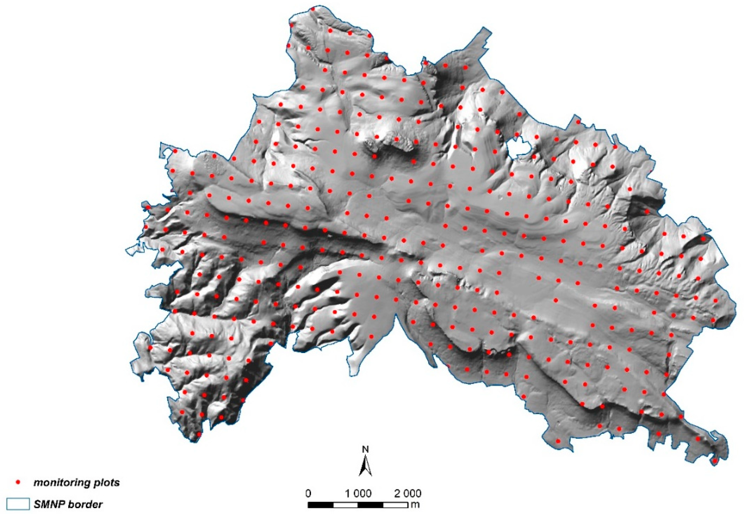
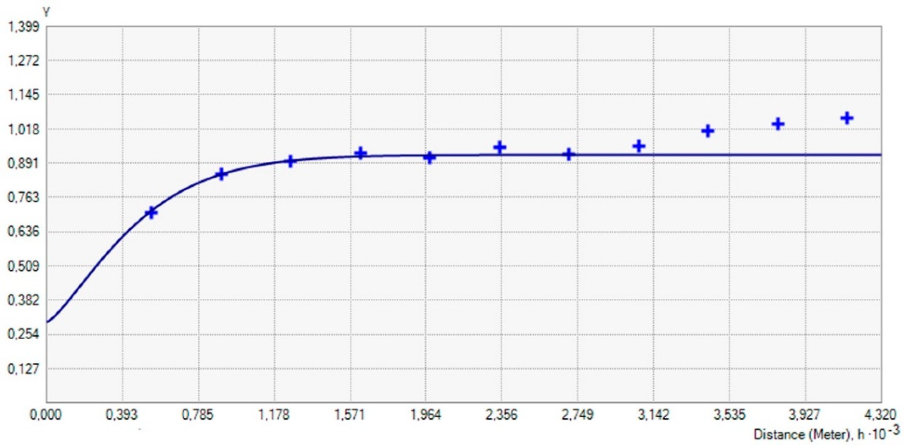
The PMNet grid comprised 403 monitoring plots arranged in a regular square grid. Due to the lack of technical feasibility of soil sampling in certain areas, only 387 plots were included in the analysis (Figure 2). The geostatistical model for PMNet was developed using the simple kriging method, for which the spatial dependence was best described by a stable curve algorithm. The autocorrelation range for Pb concentration exceeded 1000 m. The nugget value was 0.101, which may suggest the presence of small-scale spatial variations. In turn, the semi-variance values for PMNet indicate the highest spatial autocorrelation as compared to the other networks (RMNet, REMNet).
The autocorrelation strength was also indicated by the nugget-to-sill ratio (RNS index), which determines the ratio of the nugget value to the sill value of semi-variance. RNS is computed as (C0/(C0 + C)), where C0 is the nugget value, and C is the sill value of semi-variance.
As reported by [62,63], this ratio shows strong, moderate and weak spatial dependence in the value ranges <0.25, 0.25−0.75 and >0.75, respectively. In the case of the PMNet network, it was 0.36 (Table 2), which indicates a moderate spatial autocorrelation of Pb.
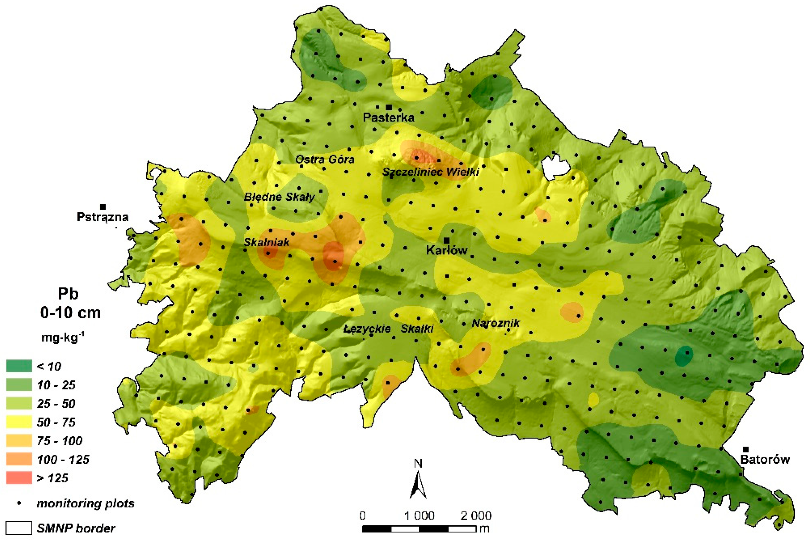
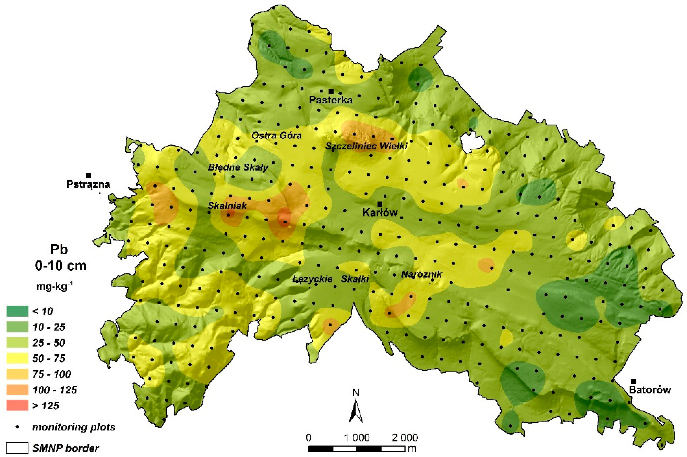
In assessing the quality of the model by cross-validation, the value of the error rate MSE was found to be close to zero and the RMSE was close to 1 (Table 3), which according to [64] attested to the correctness of the model. The prediction of the spatial distribution of Pb concentration in the 0–10 cm soil layer, developed on the basis of the geostatistical model for PMNet, is presented in Figure 3.
According to the prediction, the highest Pb values (>100 mg kg−1) were recorded in the central and western parts of the SMNP. They occurred mainly in the highest elevated areas of the mountains (i.e., in the region of Mt. Skalniak and Mt. Szczeliniec Wielki).
On the other hand, most locations showed Pb concentrations close to the median (Table 1). These areas covered mainly the eastern part (Batorowo area) as well as the northern part, but they also appeared in the central region of the area. In the eastern region, Pb concentrations did not exceed 10 mg kg−1.
3.2. Reduced Monitoring Network (RMNet)
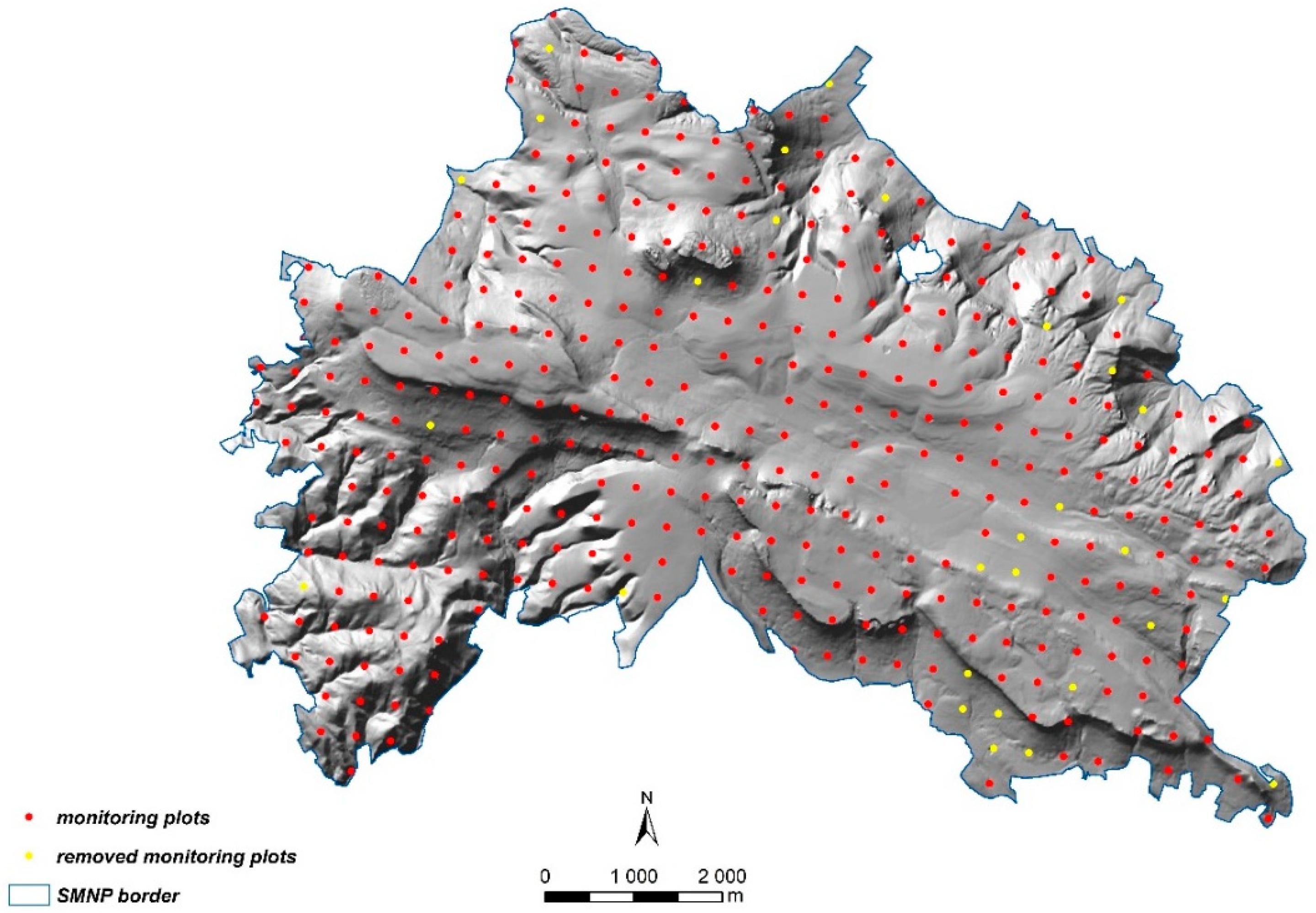
Based on the criteria defined in Section 2.3, the PMNet structure was reduced by 30 monitoring plots. Finally, the total number of plots in RMNet was 357. Most plots were removed from the northern and eastern region (Figure 4).
As in the case of PMNet, the geostatistical model for RMNet was developed using the simple kriging method. Spatial autocorrelation was best represented by a stable curve algorithm. The autocorrelation range was slightly larger than that in the model for PMNet and was more than 1160 m, but the values of nugget and partial sill of semivariance increased. Removal of the selected monitoring plots resulted in an increase in the mean distance between them and a decrease in spatial autocorrelation as against the PMNet. Similar to the PMNet model, the RNS value indicated, according to [62,63], a moderate spatial autocorrelation of Pb concentration (Table 2). Based on the MSE and RMSE errors, it was found that despite the reduction in the number of monitoring plots, the model was correctly executed (Table 3).
The prediction of spatial Pb distribution was similar to that developed for PMNet (Figure 5). There was a decrease in the range of surfaces with a predicted lead concentration of 10–20 mg kg−1 (mainly in the eastern and northern regions) and >125 mg kg−1 (Mt. Szczeliniec Wielki), whereas the areas with a predicted Pb concentration of 25–50 mg kg−1, close to the mean Pb concentration, slightly increased (Figure 5).
3.3. Reduced and Extended Monitoring Network (REMNet)
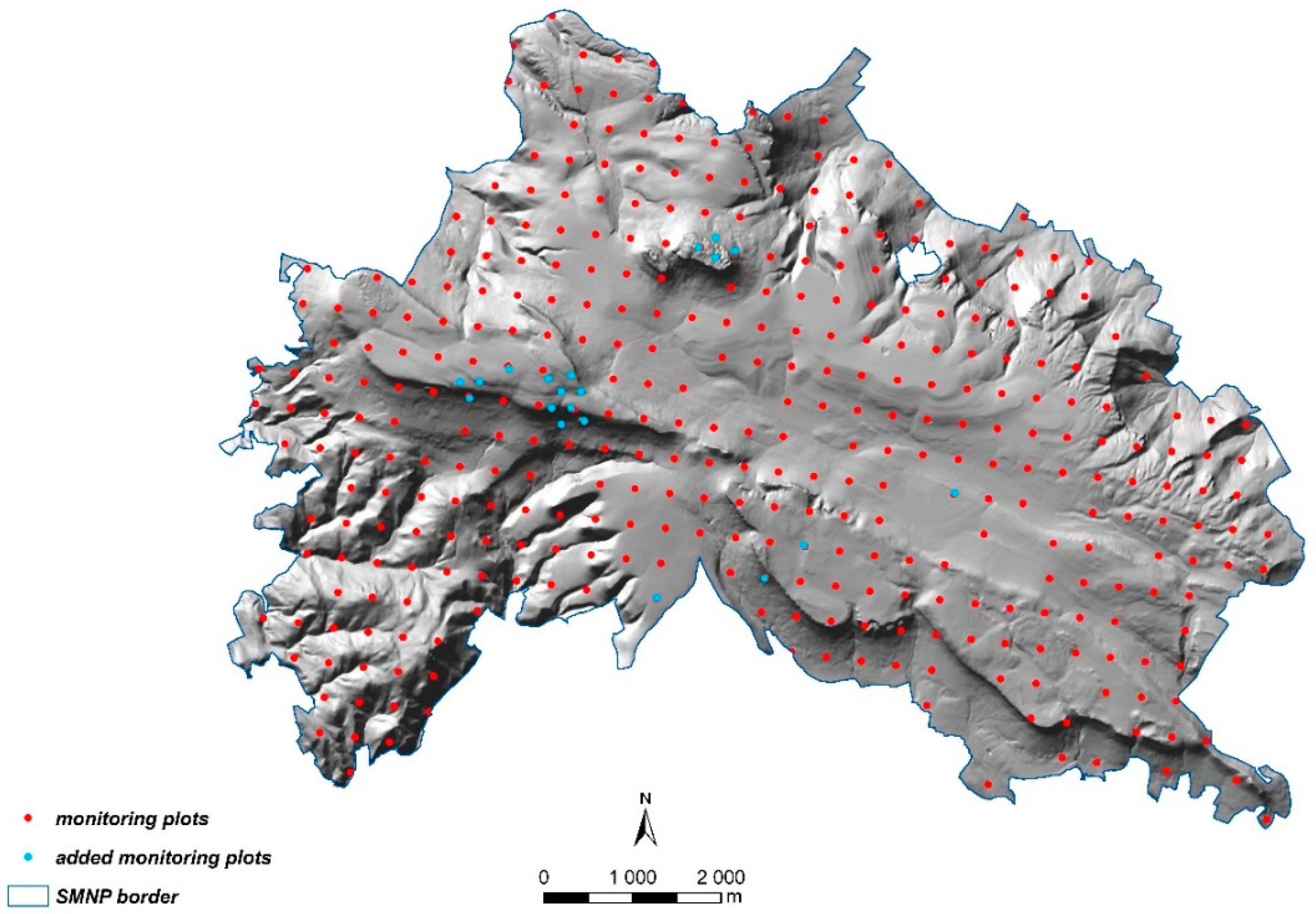
The modification of the RMNet structure according to the assumptions set out in Section 2.3 resulted in the addition of 20 new monitoring plots. Their number and location were determined by the network density analyser, taking into account an additional criterion that excluded the overlapping of the plots. The distribution of the new plots was characterised by irregularity. The largest number of new plots was located in the highest elevations (i.e., in the vicinity of Mt. Skalnik and Mt. Szczeliniec Wielki). The REMNet grid created in this manner finally comprised 377 plots (Figure 6) (i.e., 10 less than the PMNet). The simple kriging method was also used for modelling, but in this case, the spatial autocorrelation was best described by the Gaussian curve algorithm. The autocorrelation range and the values of the nugget and partial sill were similar to the model made for the RMNet. As with the RMNet, modifying the network structure resulted in an increase in the mean distance between monitoring plots and a decrease in spatial autocorrelation. Spatial autocorrelation was noticeably lower compared to the PMNet and slightly higher than the RMNet.
Similar to the models for PMNet and RMNet grids, the value of the RNS index (Table 2) indicated a moderate spatial autocorrelation of Pb concentration [62,63]. The MSE and RMSE errors (Table 3) indicated correct modelling [64].
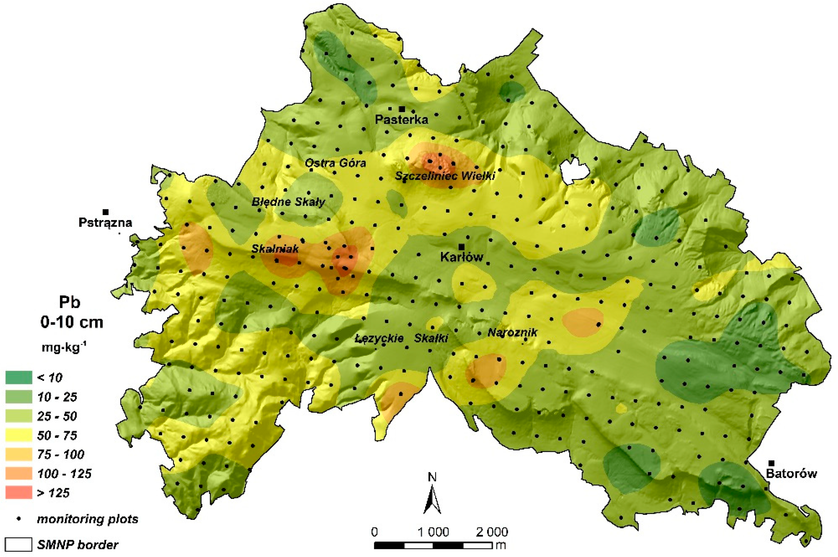
The prediction of the spatial Pb distribution for REMNet increased the share of plots with Pb concentrations ranging from 25 to 50 mg kg−1 in the central part of the area and decreased the share of areas with contents ranging from 10 to 25 mg kg−1 in the eastern part (Figure 7). The prediction of the spatial Pb distribution did not bring significant changes compared to the map developed for RMNet (Figure 5); however, it came closer again to the spatial variability reflected within the PMNet (Figure 3).
4. Discussion
The proposed concept of the evaluation and modification of a monitoring network is an original solution. As mentioned in the introduction, the procedures presented by other authors are different and based on individual solutions, however, they have a similar objective, which is the optimisation of monitoring networks used in environmental studies in terms of correct imaging of changes that may occur in broader temporal and spatial perspectives [65,66].
The geostatistical analyses conducted in this study indicated that the initial PMNet structure allowed for the effective identification of Pb distribution in SMNP soils. The spatial autocorrelation range for this element exceeded 1000 m, despite a large number of factors potentially affecting the soil variability in mountainous areas. This finding could be explained by the poor mobility of Pb in soils or its strong affinity to organic matter [4,9,16], leading to its accumulation in the topsoil layers, particularly in the forest soils. The geostatistical model for PMNet, applying the cross-validation evaluation, developed in this study with respect to RMNet and REMNet models, showed mean standardised error and root mean squared error values closest to the optimal ones (Table 3). However, it did not reach them, most likely due to the distribution of monitoring plots in a rigid square grid, where one plot represents 0.16 km2. As indicated by other authors [15,65,67], the representativeness of such large plots may be questionable in regions of high relief variability.
The main idea of the new monitoring network structures was an optimisation oriented towards minimising the number of monitoring plots while maintaining the correctness and accuracy of soil parameter imaging. Achieving this goal using geostatistical methods may translate into better economic performance and shorter time of study [68]. Both network modernisation concepts (RMNet and REMNet) meet the adopted requirements. In both cases, the number of monitoring plots was reduced (RMNet by 30, REMNet by 10), and the geostatistical models developed for them were characterised by fine correctness. The MSE and RMSE errors are close to the optimal values reported by other authors, but slightly worse compared to the parameters obtained for the initial PMNet (Table 3). The higher values of the partial sill and nugget for RMNet and REMNet are due to higher values of semivariance in the spatial autocorrelation models, potentially as a result of the change in the structure of these networks caused by reducing the number of monitoring plots under analysis, which led to an increase in the average distance between them [67,69]. The increase in the value of error(s) as far as the REMNet is concerned, may also be due to the fact that Pb contents in the points added at the last stage were not derived from the new sampling and analysis, but rather, were determined based on the original prediction map. It cannot be excluded that samples from the added points would have revealed higher local contamination, which would have affected the prediction.
The spatial variability of Pb concentration imaged in RMNet and REMNet, despite minor differences, reflected spatial dependencies that compared well to the PMNet. In the map developed for the REMNet, surfaces with high Pb concentration (>100 mg kg−1) are enlarged, suggesting poorer representativeness of some monitoring plots in the PMNet structure. Therefore, the use of the REMNet in future monitoring studies in this study area may be more beneficial for the recognition of the spatial variability of Pb concentration, but will slightly reduce workloads. An unavoidable disadvantage of this proposal is the necessity to designate new monitoring plots outside the original locations. This requirement will reduce the possibility of comparing the results in successive monitoring studies, and thus, may weaken the statistical significance of possible time-related trends.
It is worth noting that one of the alternative solutions for optimising the existing network structure with the use of geostatistical tools could be redesigning it from scratch. As far as the modelling process is concerned, the application of the kriging method makes it possible to recognise the spatial variability structure and to use it to produce the sampling design [70]. As indicated by [71], the maximum standard error of a kriged estimate is a reasonable measure of the goodness of the sampling design. In this case, using a regular triangular grid as the sampling scheme usually minimises the maximum standard error. In turn, for each assumed maximum standard error, the optimal density can be determined based on the semivariogram for the variable. However, it must be emphasised that the concept for the evaluation of the existing monitoring network presented was not intended to introduce a completely new network structure. It aimed to optimise the network with as little interference as possible of its original regular grid structure. As mentioned in Section 2.3, the network was also designed to observe other environmental components (tree stands, vegetation, lichens, etc.). Thus, the introduction of a completely new network structure just for soils would hinder the implementation of monitoring as well as the linking and interpretation of data related to all of the components assessed.
Moreover, only one parameter relating to soil contamination was applied in the current study. As far as the optimisation of the monitoring network is concerned, it is necessary to analyse at least a few key parameters relating, for example, to macroelement concentration and organic carbon pools, which are relevant for semi-natural forest reconstruction and climate-change mitigation policies, respectively. It will only be possible to present the economic calculation for the proposed method, and thus, determine the validity of its application, after performing the analyses for a larger number of parameters.
It cannot be ruled out that geostatistical analyses will provide not one, but different variants of the monitoring network structure, the merging of which will not be substantively justified. In such an event, it would be more reasonable to use distinct modifications of the network structure, separately for selected key parameters, developed according to the methodology presented for the creation of the RMNet structure. It is possible that in the case of the more mobile soil parameters, their spatial distribution might strongly vary over time, thus reducing the potential of the presented approaches (RMNet and REMNet). The RMNet approach will require more field and laboratory work but this will yield more reliable analysis results.
5. Conclusions
The use of geostatistical tools to optimise the structure of the original mountain forest soil monitoring network, which is established based on a regular square grid, resulted in a reduction in the total number of monitoring plots. Different variants of reduced monitoring networks, developed using the proposed procedure, make it possible to build correct geostatistical models characterised by slightly worse MSE and RMSE errors versus the original, regular monitoring network. The prediction of Pb concentration in soils based on the new geostatistical models changed the spatial proportions of areas in different pollution classes to a limited extent compared to the original regular network. Although the application of the geostatistical tools gave positive results, the final proposal for the optimisation of the monitoring network should include additional analyses performed using a similar method for other key soil parameters, particularly macronutrients and organic carbon pools, which are crucial for the achievement of monitoring objectives as well as for forest management and protection policies in the national park.
Author Contributions
All authors contributed to the development of the idea and authoring of the paper: Conceptualisation P.J. and C.K.; methodology P.J.; writing—original draft P.J.; writing—review and editing C.K. All authors have read and agreed to the published version of the manuscript.
Funding
This work was co-financed by the Ministry of Higher Education and Science of Poland, project MNiSW N R09 0029 04/2008 and a statute project of the Wrocław University of Environmental and Life Sciences, Institute of Soil Science and Environmental Protection from a subsidy of the Ministry of Education and Science of Poland.
Institutional Review Board Statement
Not applicable.
Informed Consent Statement
Not applicable.
Data Availability Statement
The study did not report any data.
Acknowledgments
The authors wish to thank A. Bogacz, B. Gałka, B. Łabaz and J. Waroszewski, who were included in the development of the soil studies in the Stolowe Mountains National Park.
Conflicts of Interest
The authors declare no conflict of interest.
Appendix A
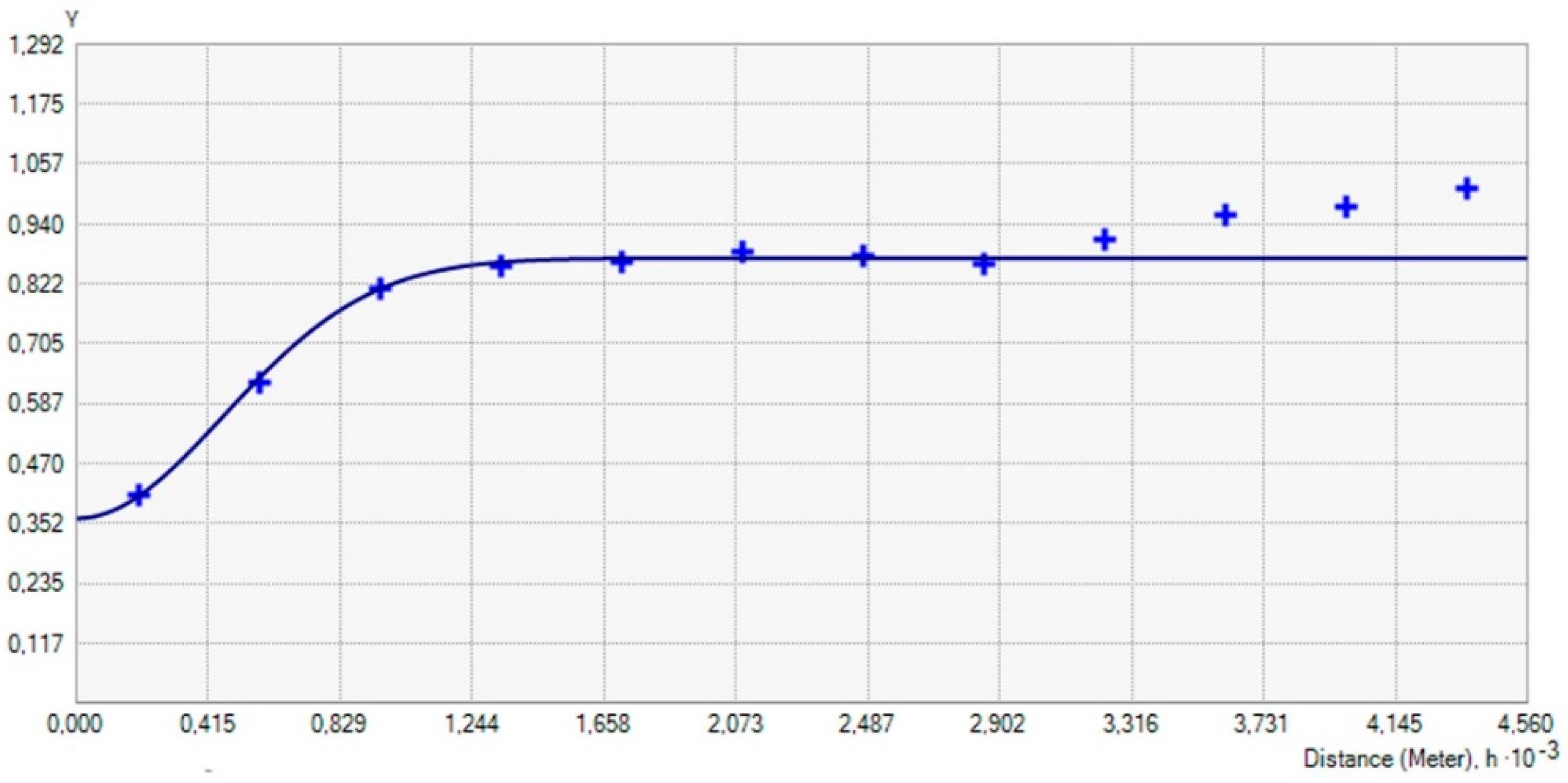
Figure A1.
Experimental semivariogram (symbols) and models (line) for total concentration of Pb in the topsoil layer—PMNet.
Figure A1.
Experimental semivariogram (symbols) and models (line) for total concentration of Pb in the topsoil layer—PMNet.

Figure A2.
Experimental semivariogram (symbols) and models (line) for total concentration of Pb in the topsoil layer—RMNet.
Figure A2.
Experimental semivariogram (symbols) and models (line) for total concentration of Pb in the topsoil layer—RMNet.

Figure A3.
Experimental semivariogram (symbols) and models (line) for total concentration of Pb in the topsoil layer—REMNet.
Figure A3.
Experimental semivariogram (symbols) and models (line) for total concentration of Pb in the topsoil layer—REMNet.

References
- Skiba, S. Soil as a link between abiotic and biotic environment. Rocz. Bieszcz. 2017, 25, 355–372. [Google Scholar]
- Morvan, X.; Saby, N.P.A.; Arrouays, D.; Le Bas, C.; Jones, R.J.A.; Verheijen, F.G.A.; Kibblewhite, M.G. Soil monitoring in Europe: A review of existing systems and requirements for harmonization. Sci. Total Environ. 2008, 391, 1–12. [Google Scholar] [CrossRef]
- Mazurek, R.; Kowalska, J.; Gąsiorek, M.; Zadrożny, P.; Józefowska, A.; Zaleski, T.; Orłowska, K. Assessment of heavy metals contamination in surface layers of Roztocze National Park forest soils (SE Poland) by indices of pollution. Chemosphere 2017, 168, 839–850. [Google Scholar] [CrossRef] [PubMed]
- Utermann, J.; Aydın, C.T.; Bischoff, N.; Böttcher, J.; Eickenscheidt, N.; Gehrmann, J.; König, N.; Scheler, B.; Stange, F.; Wellbrock, N. Heavy metal stocks and concentrations in forest soils. In Status and Dynamics of Forests in Germany; Wellbrock, N., Bolte, A., Eds.; Ecological Studies (Analysis and Synthesis); Springer: Cham, Switzerland, 2019; Volume 237, pp. 190–229. [Google Scholar]
- Burger, J.A.; Kelting, D.L. Soil quality monitoring for assessing sustainable forest management. In The Contribution of Soil Science to the Development of and Implementation of Criteria and Indicators of Sustainable Forest Management; Adams, M.B., Ramakrishna, K., Davidson, E.A., Eds.; SSSA Special Series; Soil Science Society of America: Madison, WI, USA, 1999; Volume 53, pp. 17–52. [Google Scholar]
- Frank, J.J.; Poulakos, A.G.; Tornero-Velez, R.; Xue, J. Systematic review and meta-analyses of lead (Pb) concentrations inenvironmental media (soil, dust, water, food, and air) reported in the United States from 1996 to 2016. Sci. Total. Environ. 2019, 694, 133489. [Google Scholar] [CrossRef]
- Suchara, I.; Sucharová, J. Current atmospheric deposition loads and their trendsin the Czech Republic determined by mapping the distribution of moss element contents. J. Atmos. Chem. 2004, 49, 503–519. [Google Scholar] [CrossRef]
- Błońska, E.; Lasota, J.; Szuszkiewicz, M.; Łukasik, A.; Klamerus-Iwan, A. Assessment of forest soil contamination in Krakow surroundings in relation to the type of stand. Environ. Earth Sci. 2016, 75, 1205. [Google Scholar] [CrossRef] [Green Version]
- Kabala, C.; Karczewska, A.; Medynska-Juraszek, A. Variability and relationships between Pb, Cu, and Zn concentrations in soil solutions and forest floor leachates at heavily polluted sites. J. Plant Nutr. Soil Sci. 2014, 177, 573–584. [Google Scholar] [CrossRef]
- Gałka, B.; Kabała, C.; Łabaz, B.; Bogacz, A. Influence of stands with diversed share of Norway spruce in species structure on soils of various forest habitats in the Stołowe Mountains. Sylwan 2014, 158, 684–694. [Google Scholar]
- Lal, R. Restoring soil quality to mitigate soil degradation. Sustainability 2015, 7, 5875–5895. [Google Scholar] [CrossRef] [Green Version]
- McHale, M.R.; Lawrence, G.B.; Siemion, J.; Bonville, D.B. Establishing a national forest soil monitoring network: Chemical variability in forest soils. In Proceedings of the American Geophysical Union, Fall Meeting 2018, Washington, DC, USA, 10–14 December 2018. Abstract #H13J-1855. [Google Scholar]
- De Vries, W.; Vel, E.; Reinds, G.J. Intensive monitoring of forest ecosystems in Europe: 1. Objectives, set-up and evaluation strategy. For. Ecol. Manag. 2003, 174, 77–95. [Google Scholar] [CrossRef]
- Karczewska, A.; Szopka, K.; Bogacz, A. Zinc and lead in forest soils of Karkonosze National Park—data for assessment of environmental pollution and soil monitoring. Pol. J. Environ. Stud. 2006, 15, 336–342. [Google Scholar]
- Junxiao, W.; Xiaorui, W.; Shenglu, Z.; Shaohua, W.; Yan, Z.; Chunfeng, L. Optimization of sample points for monitoring arable land quality by simulated annealing while considering spatial variations. Int. J. Environ. Res. Public Health 2016, 13, 980. [Google Scholar]
- Szopka, K.; Karczewska, A.; Jezierski, P.; Kabala, C. Spatial distribution of lead in the surface layers of mountain forest soils, an example from the Karkonosze National Park, Poland. Geoderma 2013, 192, 259–268. [Google Scholar] [CrossRef]
- Fleck, S.; Cools, N.; De Vos, B.; Meesenburg, H.; Fischer, R. The Level II aggregated forest soil condition database links soil physicochemical and hydraulic properties with long-term observations of forest condition in Europe. Ann. Forest Sci. 2016, 73, 945–957. [Google Scholar] [CrossRef] [Green Version]
- Eid AN, M.; Olatubara, C.O.; Ewemoje, T.A.; El-Hennawy, M.T.; Farouk, H. Spatial and seasonal assessment of physico-chemical characteristics of soil in Wadi El-Rayan lakes using GIS technique. SN Appl. Sci. 2021, 3, 146. [Google Scholar] [CrossRef]
- Prietzel, J.; Falk, W.; Reger, B.; Uhl, E.; Pretzsch, H.; Zimmermann, L. Half a century of Scots pine forest ecosystem monitoring reveals long?term effects of atmospheric deposition and climate change. Glob. Chang. Biol. 2020, 26, 5796–5815. [Google Scholar] [CrossRef] [PubMed]
- Szopka, K.; Kabala, C.; Karczewska, A.; Jezierski, P.; Bogacz, A.; Waroszewski, J. The pools of soil organic carbon accumulated in the surface layers of forest soils in the Karkonosze Mountains, SW Poland. Soil Sci. Annu. 2016, 67, 46–56. [Google Scholar] [CrossRef] [Green Version]
- Rutkowski, P.; Diatta, J.; Konatowska, M.; Andrzejewska, A.; Tyburski, Ł.; Przybylski, P. Geochemical referencing of natural forest contamination in Poland. Forests 2020, 11, 157. [Google Scholar] [CrossRef] [Green Version]
- Lu, Z. Construction of soil environment information management platform based on ArcGIS. IOP Conf. Ser. Earth Environ. Sci. 2020, 546, 032039. [Google Scholar]
- Łyszczarz, S.; Błońska, E.; Lasota, J. The application of the geo-accumulation index and geostatistical methods to the assessment of forest soil contamination with heavy metals in the Babia Góra National Park (Poland). Arch. Environ. Prot. 2020, 46, 69–79. [Google Scholar]
- Obade, V.; Lal, R. Assessing land cover and soil quality by remote sensing and geographical information systems (GIS). Catena 2013, 104, 77–92. [Google Scholar] [CrossRef]
- Moore, F.; Sheykhi, V.; Salari, M.; Bagheri, A. Soil quality assessment using GIS-based chemometric approach and pollution indices: Nakhlak mining district, Central Iran. Environ. Monit. Assess. 2016, 188, 214. [Google Scholar] [CrossRef]
- Zhu, X. GIS for Environmental Applications: A Practical Approach; Routledge: Abingdon, NY, USA, 2016; p. 471. [Google Scholar]
- O’Riordan, T. Environmental Science for Environmental Management, 2nd ed.; Taylor & Francis: Germantown, NY, USA, 2000; p. 519. [Google Scholar]
- Wright, D.J.; Harder, C. GIS for Science: Applying Mapping and Spatial Analytics; ESRI Press: Redlands, CA, USA, 2019; p. 252. [Google Scholar]
- Hernandez-Stefanoni, J.L.; Ponce-Hernandez, R. Mapping the spatial variability of plant diversity in a tropical forest: Comparison of spatial interpolation methods. Environ. Monit. Assess. 2006, 117, 307–334. [Google Scholar] [CrossRef] [PubMed]
- Kimsey, M.J.; Laing, L.E.; Anderson, S.M.; Bruggink, J.; Campbell, S.; Diamond, D.; Vaughan, R. Soil Mapping, Monitoring, and Assessment. In Forest and Rangeland Soils of the United States Under Changing Conditions; Springer: Cham, Switzerland, 2020; pp. 169–188. [Google Scholar]
- Trofymchuk, O.; Klymenko, V.; Anpilova, Y.; Sheviakina, N.; Zagorodnia, S. The aspects of using GIS in monitoring of environmental components. In Proceedings of the International Multidisciplinary Scientific GeoConference: SGEM, Albena, Bulgaria, 16–25 August 2020; Volume 20, pp. 581–588. [Google Scholar]
- Karczewska, A.; Bogacz, A.; Kabała, C.; Szopka, K.; Duszyńska, D. Methodology of soil monitoring in a forested zone of the Karkonosze National Park with reference to the diversity of soil properties. Polish J. Soil Sci. 2006, XXXIX/2, 117–129. [Google Scholar]
- Wawrzoniak, J. (Ed.) The Health Status of Forests in Poland in 2018; Forest Research Institute, Department of Forest Resources Management: Sękocin Stary, Poland, 2019; p. 66. [Google Scholar]
- Bojko, O.; Kabala, C. Transformation of physicochemical soil properties along a mountain slope due to land management and climate changes-a case study from the Karkonosze Mountains, SW Poland. Catena 2016, 140, 43–54. [Google Scholar] [CrossRef]
- Szopka, K.; Karczewska, A.; Kabala, C. Mercury accumulation in the surface layers of mountain soils: A case study from the Karkonosze Mountains, Poland. Chemosphere 2011, 83, 1507–1512. [Google Scholar] [CrossRef] [PubMed]
- Raj, A.; Zientarski, J. Monitoring of forest ecosystems in the Karkonosze National Park. Opera Corcon. 2007, 44, 423. [Google Scholar]
- Pennock, D.J. Designing field studies in soil science. Can. J. Soil Sci. 2004, 84, 1–10. [Google Scholar] [CrossRef] [Green Version]
- O’Harea, M.T.; Gunna, I.D.M.; Critchlow-Wattonb, N.; Guthrieb, R.; Taylorb, C.; Chapmana, D.S. Fewer sites but better data? Optimising the representativeness and statistical power of a national monitoring network. Ecol. Indic. 2020, 114, 106321. [Google Scholar]
- De Gruijter, J.; Brus, D.; Bierkens, M.; Knotters, M. Sampling for Natural Resource Monitoring; Springer: Berlin/Heidelberg, Germany; New York, NY, USA, 2006; p. 326. [Google Scholar]
- Sampling Design Part 1—Application. Contaminated Land Guidelines; State of New South Wales and the NSW Environment Protection Authority, NSW EPA: Parramatta, Australia, 2020; p. 84.
- Nordgaard, A.; Correll, R. Sampling Strategies. In Integrated Analytical Approaches for Pesticide Management; Maestroni, B., Cannavan, A., Eds.; Academic Press Elsevier: Cambridge, MA, USA, 2018; pp. 31–46. [Google Scholar]
- Black, H.; Bellamy, P.; Creamer, R.; Elston, D.; Emmett, B.; Frogbrook, Z.; Hudson, G.; Jordan, C.; Lark, M.; Lilly, A.; et al. Design and Operation of a UK Soil Monitoring Network; Science Report—SC060073; Environment Agency: Bristol, UK, 2008; p. 218. [Google Scholar]
- Lindenmayer, D.B.; Likens, G.E. Adaptive monitoring: A new paradigmfor long term research and monitoring. Trends Ecol. Evol. 2009, 24, 482–486. [Google Scholar] [CrossRef]
- Yanguo, T.; Jin, W.; Sijin, L.; Yeyao, W.; Xudong, J.; Liuting, S. Soil and soil environmental quality monitoring in China: A review. Environ. Int. 2014, 69, 177–199. [Google Scholar]
- Xiao-Ni, H.; Hong, L.; Dan-Feng, S.; Lian-Di, Z.; Bao-Guo, L. Combining geostatistics with Moran’s I analysis for mapping soil heavy metals in Beijing, China. Int. J. Environ. Res. Public Health 2012, 9, 995–1017. [Google Scholar]
- Arrouays, D.; Marchant, B.P.; Saby, N.P.A.; Meersmans, J.; Orton, T.G.; Martin, M.P.; Bellamy, P.H.; Lark, R.M.; Kibblewhite, M. Generic Issues on Broad-Scale Soil Monitoring Schemes: A Review. Pedosphere 2012, 22, 456469. [Google Scholar] [CrossRef]
- Hofman, C.K.; Brus, D.J. How many sampling points are needed to estimate the mean nitrate-N content of agricultural fields? A geostatistical simulation approach with uncertain variograms. Geoderma 2021, 385, 114816. [Google Scholar] [CrossRef]
- Guo, L.; Linderman, M.; Shi, T.; Chen, Y.; Duan, L.; Zhang, H. Exploring the sensitivity of sampling density in digital mapping of soil organic carbon and its application in soil sampling. Remote Sens. 2018, 10, 888. [Google Scholar] [CrossRef] [Green Version]
- Migoń, P.; Latocha, A.; Parzóch, K.; Kasprzak, M. Contemporary geomorphic system of the Stolowe Mountains. In Geo-Ecological Conditions of the Stolowe Mountains National Park; Chodak, T., Ed.; Wind: Wroclaw, Poland, 2011; pp. 1–52. [Google Scholar]
- Wojewoda, J. Geological structure of the PNGS area. In Nature of the Stołowe Mountains National Park; Witkowski, A., Pokryszko, P.M., Ciężkowski, W., Eds.; PNGS Publishing: Kudowa Zdrój, Poland, 2008; p. 404. [Google Scholar]
- Pawlak, W. Atlas of Lower and Opole Silesia, 2nd ed.; Wroclaw University: Wroclaw, Poland, 2008. [Google Scholar]
- Kabała, C.; Chodak, T.; Bogacz, A.; Łabaz, B.; Jezierski, P.; Gałka, B.; Kaszubkiewicz, J.; Glina, B. Spatial variability of soils and habitats in the Stołowe Mountains National Park. In Geoecological Conditions of the Stołowe Mountains National Park Natural Environment; Chodak, T., Kabała, C., Kaszubkiewicz, J., Migoń, P., Wojewoda, J., Eds.; WIND Publishing: Wrocław, Poland, 2011; pp. 141–168. [Google Scholar]
- Jędryszczak, E.; Miścicki, S. Lasy Parku Narodowego Gór Stołowych. Szceliniec 2001, 4, 79–103. [Google Scholar]
- Świerkosz, K.; Boratyński, A. Chorological and synanthropodynamical analysis of trees and shrubs of the Stołowe Mts. (Middle Sudety). Dendrobiology 2002, 48, 75–85. [Google Scholar]
- Labaz, B.; Galka, B.; Bogacz, A. Factors influencing humus forms and forest litter properties in the mid-mountains under temperate climate of southwestern Poland. Geoderma 2014, 230, 265–273. [Google Scholar] [CrossRef]
- National Geoportal. Available online: https://mapy.geoportal.gov.pl/imap/Imgp_2.html?locale=pl&gui=new&sessionID=4943882 (accessed on 19 January 2021).
- Miścicki, S.; Nowicka, E. Measurement of forest resources using permanent concentric sample plots—Problems and attempts at their solving. Sylwan 2007, 151, 15–26. [Google Scholar]
- Regulation of the Ministry of Environment (Poland) on the Method of Assessing the Pollution of the Land Surface. Available online: http://isap.sejm.gov.pl/isap.nsf/DocDetails.xsp?id=WDU20160001395 (accessed on 13 January 2021).
- Isaaks, E.H.; Srivastava, R.M. An Introduction to Applied Geostatistics; Oxford University Press: New York, NY, USA, 1989; p. 398. [Google Scholar]
- Kabata-Pendias, A.; Pendias, H. Pierwiastki Śladowe w Glebie i Roślinach; CRC Press: Boca Raton, FL, USA, 2011; p. 365. [Google Scholar]
- El-Sayed, E.O. Improving the prediction auccuracy of oil mapping through geostatistics. Int. J. Geosci. 2012, 3, 574–590. [Google Scholar]
- Wu, W.; Xie, D.T.; Liu, H.B. Spatial variability of soil heavy metals in the three gorges area: Multivariate and geostatistical analyses. Environ. Monit Assess. 2009, 157, 63–71. [Google Scholar] [CrossRef] [PubMed]
- Kerry, R.; Oliver, K.O. Determining nugget:sill ratios of standardized variograms from aerial photographs to krige sparse soil data. Precis. Agric. 2008, 9, 33–56. [Google Scholar] [CrossRef]
- Fischer, M.M.; Getis, A. (Eds.) Handbook of Applied Spatial Analysis: Software Tools, Methods and Applications; Springer: Berlin, Germany, 2010; pp. 125–134. [Google Scholar]
- Flatman, G.T.; Yfantis, A.A. Geostatistical strategy for soil sampling: The survey and the census. Environ. Monit. Assess. 1984, 4, 335–349. [Google Scholar] [CrossRef]
- Hu, B.; Zhou, Y.; Jiang, Y.; Ji, W.; Fu, Z.; Shao, S.; Li, S.; Huang, M.; Zhou, L.; Shi, Z. Spatio-temporal variation and source changes of potentially toxic elements in soil on a typical plain of the Yangtze River Delta, China (2002–2012). J. Environ. Manag. 2020, 271, 110943. [Google Scholar] [CrossRef] [PubMed]
- Van Groenigen, J.W.; Siderius, W.; Stein, A. Constrained optimisation of soil sampling for minimisation of the kriging variance. Geoderma 1999, 87, 239–259. [Google Scholar] [CrossRef]
- Webster, R.; Olivier, M.A. Geostatistics for Environmental Scientists, 2nd ed.; John Wiley & Sons Ltd.: Chichester, UK, 2007; p. 317. [Google Scholar]
- Krivoruchko, K. Spatial Statistical Data Analysis for GIS Users; Esri Press: Redlands, CA, USA, 2011; p. 928. [Google Scholar]
- Mmcbratney, A.B.; Webster, R. Choosing functions for semi-variograms of soil properties and fitting them to sampling estimates. J. Soil Sci. 1986, 37, 617–639. [Google Scholar] [CrossRef]
- Mmcbratney, A.B.; Webster, R.; Burgess, T.M. The design of optimal sampling schemes for local estimation and mapping of regionalized variables—I. Comput. Geotcitnces 1981, 7, 331–334. [Google Scholar]
Figure 1.
Location of the study area on a digital elevation model (DEM) map. DEM data acquired from light detection and ranging (LIDAR) [56].
Figure 1.
Location of the study area on a digital elevation model (DEM) map. DEM data acquired from light detection and ranging (LIDAR) [56].
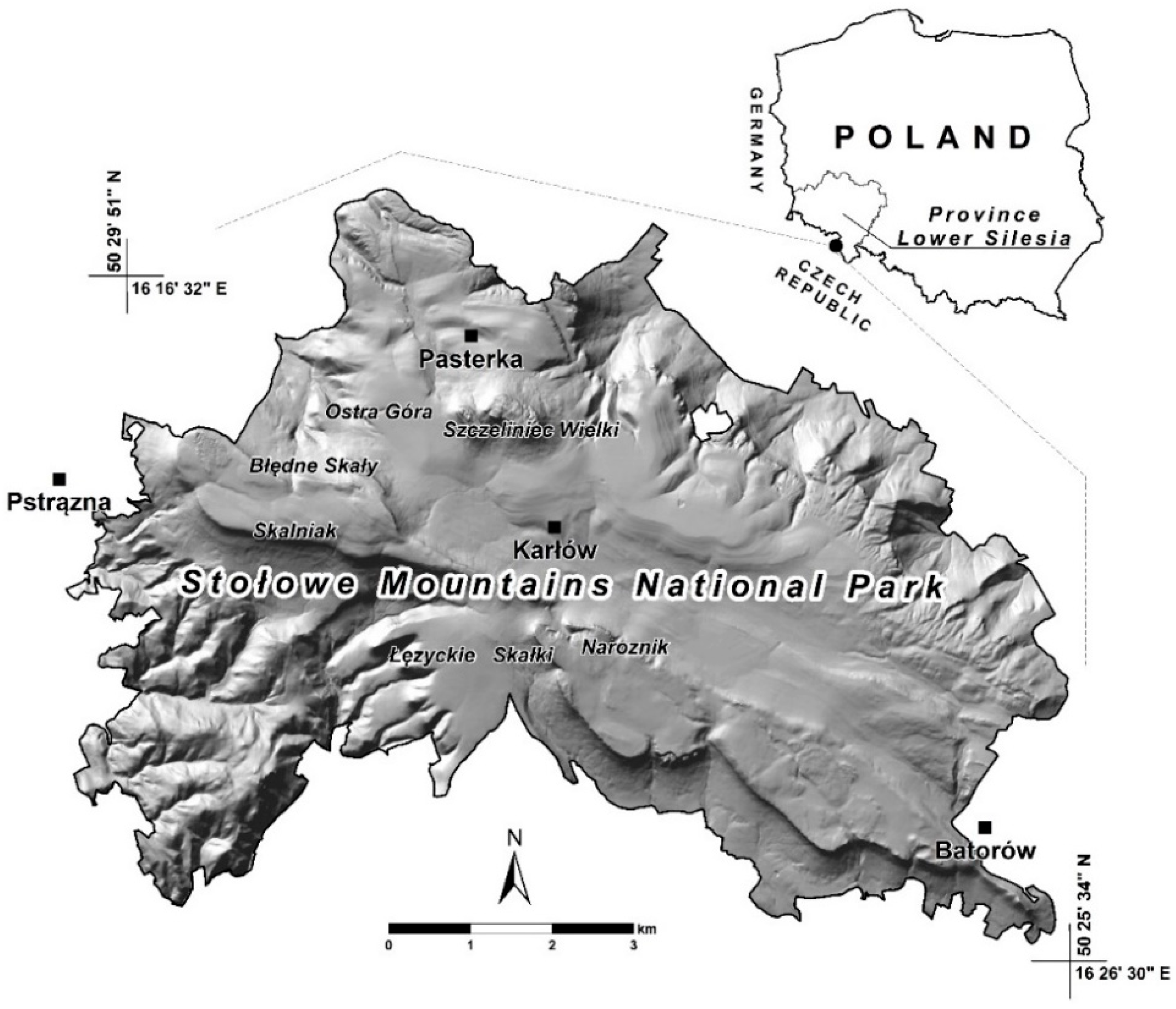
Figure 2.
Location of the 387 plots of the primary monitoring network (PMNet).

Figure 3.
Prediction map of the spatial Pb distribution, developed by simple kriging for the primary monitoring network (PMNet).
Figure 3.
Prediction map of the spatial Pb distribution, developed by simple kriging for the primary monitoring network (PMNet).

Figure 4.
Location of 357 plots (red circles) in the reduced monitoring network (RMNet). Yellow circles represent removed monitoring plots.
Figure 4.
Location of 357 plots (red circles) in the reduced monitoring network (RMNet). Yellow circles represent removed monitoring plots.

Figure 5.
Prediction map of the spatial Pb distribution, developed by simple kriging for the reduced monitoring network (RMNet).
Figure 5.
Prediction map of the spatial Pb distribution, developed by simple kriging for the reduced monitoring network (RMNet).

Figure 6.
Location of 377 plots (red and blue circles) in the reduced and extended monitoring network (REMNet). Blue circles represent added monitoring plots.
Figure 6.
Location of 377 plots (red and blue circles) in the reduced and extended monitoring network (REMNet). Blue circles represent added monitoring plots.

Figure 7.
Prediction map of the spatial Pb distribution, developed by simply kriging for the reduced and extended monitoring network (REMNet).
Figure 7.
Prediction map of the spatial Pb distribution, developed by simply kriging for the reduced and extended monitoring network (REMNet).


Table 1.
Statistical parameters characterizing variability of total Pb concentration in the soils of SMNP (data source [52]).
Table 1.
Statistical parameters characterizing variability of total Pb concentration in the soils of SMNP (data source [52]).
| N | Minimum | Maximum | Mean | Median | Standard Deviation |
|---|---|---|---|---|---|
| mg kg−1 | |||||
| 387 * | 3.5 | 219 | 46.6 | 41.0 | 28.6 |
* Due to the lack of technical feasibility of soil sampling in certain areas, only 387 of the 403 plots were included in the analysis.
Table 2.
Semivariogram model parameters for analysed monitoring networks.
| Monitoring Network | Model * | Number of Samples | Nugget | Partial Sill | Range, m | RNS |
|---|---|---|---|---|---|---|
| (C0) | (C0 + C) | (A0) | C0/(C0 + C) | |||
| PMNet | stable | 387 | 0.101 | 0.182 | 1002 | 0.36 |
| RMNet | stable | 357 | 0.301 | 0.621 | 1162 | 0.33 |
| REMNet | gaussian | 377 | 0.362 | 0.510 | 1130 | 0.42 |
* Graphs of semivariograms in Appendix A.
Table 3.
Model errors for analysed monitoring networks.
| Monitoring Network | MSE | RMSE |
|---|---|---|
| Mean Standardized Error | Root Mean Squared Error | |
| PMNet | −0.014 | 1.009 |
| RMNet | −0.025 | 1.000 |
| REMNet | 0.023 | 1.011 |
Publisher’s Note: MDPI stays neutral with regard to jurisdictional claims in published maps and institutional affiliations. |
© 2021 by the authors. Licensee MDPI, Basel, Switzerland. This article is an open access article distributed under the terms and conditions of the Creative Commons Attribution (CC BY) license (http://creativecommons.org/licenses/by/4.0/).
Share and Cite
MDPI and ACS Style
Jezierski, P.; Kabala, C. Geostatistical Tools to Assess Existing Monitoring Network of Forest Soils in a Mountainous National Park. Forests 2021, 12, 333. https://doi.org/10.3390/f12030333
AMA Style
Jezierski P, Kabala C. Geostatistical Tools to Assess Existing Monitoring Network of Forest Soils in a Mountainous National Park. Forests. 2021; 12(3):333. https://doi.org/10.3390/f12030333
Chicago/Turabian StyleJezierski, Pawel, and Cezary Kabala. 2021. "Geostatistical Tools to Assess Existing Monitoring Network of Forest Soils in a Mountainous National Park" Forests 12, no. 3: 333. https://doi.org/10.3390/f12030333
Note that from the first issue of 2016, this journal uses article numbers instead of page numbers. See further details here.