
Value of a Flexible Forest Harvest Decision with Short Period Forest Carbon Offsets: Application of a Binomial Option Model


1
School of Forest, Fisheries, and Geomatics Sciences, University of Florida, P.O. Box 110410, Gainesville, FL 32611, USA
2
Department of Forest Engineering, Resources and Management, Oregon State University, Corvallis, OR 97331, USA
3
CAPE Economic Research and Consulting, Iyana Ipaja 01234, Nigeria
*
Author to whom correspondence should be addressed.
Forests 2022, 13(11), 1785; https://doi.org/10.3390/f13111785
Submission received: 27 September 2022
/
Revised: 26 October 2022
/
Accepted: 27 October 2022
/
Published: 28 October 2022
(This article belongs to the Special Issue Advances in Decision Support for Forest Management and Policy Formulation)
Abstract
:Forest carbon offset programs have suffered from low landowner uptake, in large part to their long duration. A recent innovation in forest carbon offsets is the use of short period delays to harvest, which extend the rotation age of the stand beyond what is optimal for timber alone and increase sequestered carbon. Here, we assess the economic value of a short period delay “option pricing” in forest harvest with price uncertainty using a binomial option approach, accounting both for timber and carbon. Results from an option pricing model showed that landowners can generate considerably higher revenue with managerial flexibility along with the additional revenue from carbon offset programs. These results can help forest landowners make proper ownership decisions to withstand the risk and uncertainty associated with stumpage prices, while benefiting from carbon offset revenues.
1. Introduction
Forest management decisions typically involve a long planning horizon that can span several decades. This starts from initial site preparation to the final harvest over a single rotation and usually follows the same cycle again with the start of the next forest stand rotation. However, with the completion of each rotation, management decisions can be made based on the expectation of certain future outcomes. Given the long-time horizon, this involves making present investment decisions based on sometimes highly uncertain future returns, leading to a very complex valuation task. As such, the proper understanding of the economic value of the forest is crucial for forest landowners and managers to make effective decisions. The use of traditional deterministic analysis methods such as discounted cash flow techniques assumes that future decisions are made with perfect foresight. These approaches provide estimate values that can be used to inform the selection of an optimal land management decision and possess a varying level of usefulness depending on management objectives and capital constraints.
Using deterministic biological and economic parameters, these methods help forest managers evaluate the financial implication of different management decisions and allow for comparison with other possible alternatives. While these generally accepted methods are widely applied, they are very limited in certain regards [1]. One important limitation is that they fail to account for managerial flexibility to dynamically address the challenges (e.g., disturbance risks) and opportunities (e.g., stumpage price increases) associated with forest production in a system that is in constant flux [2]. Forest management choices are long-term decisions that face various uncertainties such as timber prices, interest rates, natural hazards, and insect attacks that can change the preferred forest management decisions. To address this issue, several methods have been developed and applied in natural resource management contexts; these methods include stochastic dominance analysis, downside risk models, mean-variance analysis, reservation price strategy, robust optimization, and option pricing model [3,4,5,6,7].
In terms of the economic sustainability of the forest enterprise, the forest harvesting decision is perhaps the most important and major management choices made by forest landowners [8]. Determination of when to harvest and subsequently regenerate the forest directly influences the economic value of forest products derived from the forest stand. With price uncertainty, making these decisions should be adaptive, allowing landowners to adjust as new information is available [9]. As revenue from the final harvest usually represents the major proportion of the total revenue (e.g., versus revenues from thinning), price-responsive harvesting decisions can considerably increase the revenue generated during the rotation. However, by lengthening the rotation age, the landowners need to consider the higher risk of fire, storm, and pests [10]. This increased value of production due to the availability of managerial flexibility to delay harvest is referred to as the option value. This option value represents the production value added due to the avoidance of unprofitable and irreversible investments [2].
The more limited, traditional discounted cash flow methods do not account for dynamic management choices that landowners can make to increase the economic value of forest production; hence, they lead to underestimates of forest production value. The real options pricing model is one such model that can incorporate managerial flexibility and capture the economic value of this flexibility. In this model, forest landowners can defer their management decision at any point in time based on the currently available information [11,12]. The additional value derived from this managerial flexibility means that real option values are always greater than or equal to value estimates from traditional discounted methods [11], with the estimates diverging more as uncertainty increases and as the predicted future departs from realized outcomes. Likewise, the convergence of values happens under two conditions; the absence of uncertainty and the real option (to exercise managerial flexibility) has expired [12]. In the absence of price uncertainty, there is no advantage of deferring harvest. Likewise, when forest landowners can no longer delay harvest, the real option has reached its expiration date.
The application of the real options pricing model to estimate the economic valuation of forest production is not entirely new. Most of the early research in this area focused on developing a real options model to estimate the optimal rotation age under stochastic timber prices [3,13,14]. These studies used two main models for their analysis: the time-continuous Black-Scholes model [7], where timber prices follow a Geometric Brownian motion process, and the time-discrete binomial model [15], where timber prices follow a binomial process. Additional studies extended the modeling application domain to include harvesting cost [16], risk of natural hazards [5,17], stationarity of price process [5], stochastic dynamic programming [1], mean-reverting price process [18,19], a two-option approach with constraints of cost over time delay [20], and time-continuous harvest decisions [21]. Apart from using the real options model to estimate the optimal rotation age, this model has also been used to develop optimal thinning strategies [22], valuation of delaying regeneration and timber processing plant expansion [10], assessment of forest concessions [23], and understanding timber market conditions for evaluating timberland investment and management opportunities [24].
The expected stumpage prices help forest landowners evaluate the returns that can be obtained from the final harvests in the future. As timber prices are always changing, determining future stumpage, and using them to make investment decisions requires proper decision-making tools. Real option models provide landowners the opportunity to use timber price volatility in the forest valuation analysis to help maximize their net returns by incorporating the flexibility to harvest when the timber prices are higher and delaying harvest when the prices are lower.
Of increasing importance is the ability to model the value of forest carbon offsets. Together with timber benefits, forest landowners can also increase their revenue through enrollment in voluntary carbon offset programs. Increase in carbon sequestration programs–such as Verra, American Carbon Registry, and Climate Action Reserve in the US has provided an opportunity to landowners to generate additional revenue by deferral in harvest and retention of forest growth relative to the harvest at deterministic rotation age [25]. Through these programs, forest landowners can engage in improved forest management activities that include deferred harvesting to achieve emission reductions that exceed the baseline. This baseline can be represented as the harvesting scenario to maximize the deterministic expected returns. This represents the additionality that is required by offset programs to show that the reduction of carbon emissions from improved forest management activity is higher than the reduction of carbon emissions without the implementation of such activities [26].
Several studies used integrated approach to evaluate the influence of carbon valuation in conjunction with timber value for forest production over the last two decades [27,28,29,30,31,32]. However, these studies reflect the programmatic realities of the day in terms of carbon offset program rules and features (e.g., very long contracts—100 years in some cases). Several studies have applied the real option model to the financial performance of managing forests with carbon payments. Ref. [33] was the first to use real options to evaluate the optimal rotation age under different carbon payment schemes using stochastic timber and carbon prices; and others have used real options to evaluate the impact of carbon credit payment schemes on forest management decisions [34,35,36,37]. All these studies valued carbon based on the carbon sequestration in the forest from plantation up to the final harvest.
Here, we contribute to the real options literature by examining the option value of delaying harvesting and regeneration of southern pine forests and include carbon offsets for short period delays in harvest. Over 57% of the timberland area in the southern United States is owned by non-industrial private forest owners [38]. Although profit maximization is not the main goal for these private landowners [39], an increase in the estimated net returns from forest production can influence land-use decisions. For example, a rise in net returns from forest production can be effective encourage forest landowners to retain their existing forest lands [40,41] and not convert to alternative uses such as cropland. Ref. [42] showed through their land-use change model of the South-Central United States that a continued increase in stumpage prices can increase the private timberland acreage in the region by 2020. Thus, using real options analysis for their forest valuation will suit their objectives. Furthermore, there is a potential for generating additional revenue through enrollment into carbon offset programs for delaying harvest and regeneration. Additionally, carbon incentive can help reduce the economic risk of natural disturbances from longer rotation age [10].
In this study, we evaluate the added value of southern pine forests by accounting for carbon benefits, given the managerial flexibility of delaying harvest, under the option pricing method. In contrast to the previous studies that evaluated the impact of carbon valuation on forest management decisions, this study will evaluate the carbon valuation under a short period delay carbon offset scheme. In our model, forest landowners only earn carbon benefits for the period of delayed harvest rather than for the carbon sequestered from plantation up to the final harvest. This is consistent with the additionality requirement of an emerging current carbon offset program available in the US run by the Natural Capital Exchange (NCX) that incentivizes short-term harvest deferral [43]. We employ the Faustmann formula [44] as a benchmark to determine the land expectation value and the optimal rotation ages of a stand of slash pine under multiple management scenarios. Slash pine (Pinus elliottii) was chosen given its status as a dominant commercial pine species in the south. We then employ the binomial option pricing model to evaluate the added value of delaying harvest and regeneration for each scenario, considering the potential carbon payments from voluntary carbon offset programs. Harvest delays of up to 15 years are assessed.
2. Materials and Methods
2.1. Binomial Option Model
Binomial option approach is the simplest form of option pricing analysis as it requires less rigorous mathematical background and skill to use [11]. Cox et al. (1979) and Rendleman (1979) independently developed a two-state discrete-time model to estimate the numerical analysis of option values [15,45]. This model introduces stochastic prices through discrete time steps, where it moves into upstate and downstate [11]. This allows this model to estimate the American call option, where the option can be exercised at any time of investment maturity. This means that investor will have option to sell the underlying asset when the price moves favorably any time before or including the expiration date.
In the binomial options model, the price of the underlying commodity can move in two directions: the price can either go up with the probability π or go down with the probability (1 − π). The price moves in two directions continuously over the life of the option. The up and down movement of the binomial process can be represented as follows:
where is the upward multiplicative factor, is the downward multiplicative factor, is the probability of upward movement, is the volatility of stochastic prices, is the time interval or the step size, and is the risk-free interest rate [15]. The upward and downward movements are used to develop a binomial tree as seen in Figure 1, where is the value of the investment.
Using the binomial process tree, the price of an option is estimated by going backward, where the option value is estimated for each binomial price node one step at a time. The option value is estimated using a recursive backward estimation which can be represented as:
where is the investment value at time , is the investment cost, and is the value of the option at time t [11]. The option value of the investment is estimated by solving the Equation (4) recursively until = 0.
2.2. Model Application
From a forestry perspective, we can use the Faustmann formula to model the land expectation value () of a forest stand considering timber benefits from both harvest and thinnings, and assuming constant timber prices and silvicultural costs. LEV is the value of bare land in perpetual timber production [46]. The land expectation value (LEV) over an infinite rotation horizon was estimated as [44]:
where, P is the deterministic stumpage price, Q(T) is the merchantable timber volume at time T, Pt is the deterministic net price of thinned wood, Q(t) is the amount of thinned wood, c is the production cost, and r is the real discount rate.
The modified Faustmann model that incorporates carbon benefit can be represented as [47]:
where, Ac(t) represents the economic benefits of carbon sequestration from delayed harvest. This benefit can be estimated as:
where, Pc is the price of carbon, and Cs(t) is the annual increase of net carbon stock in the stand, which represents total carbon in situ (slash pine + understory + forest floor + standing dead trees) plus total C ex situ (carbon in woody products sawtimber, chip-and-saw and pulpwood) minus total carbon lost from silvicultural activities (including transport) [48], and d represents the cost associated with enrollment into carbon offset program such as aggregator’s fee, verification fee and transaction fee [32].
Under the stochastic prices, expected LEV using the binomial option values can be estimated using Equation (4) as:
where, π represents the probability of price moving up, u is the upward multiplicative factor and d is the downward multiplicative factor.
This equation can be further modified to estimate the expected LEV with the additional economic benefit from carbon offset from delayed harvest can be represented as:
where, the first part represents the expected LEV estimated using the binomial option values and second part represents the payment for annual carbon increment from delayed harvest.
2.3. Forest Management Scenarios and Economic Data
Slash pine production under four management scenarios was evaluated in this study (Table 1). These scenarios represent typical production practices in the US South (M. Dooner, personal communication, 15 December 2017). They were developed based on direct communication with forest stakeholders in the region. These stakeholders included forest landowners, forest consultants, regional forestry professionals, representatives from forestry agencies, and forest academics. Scenario 1 and 2 represented plantations with lower planting density, no fertilization, no thinning, and managed with prescribed burns. Similarly, scenarios 3 and 4 represented forest produced with higher planting density and managed with multiple fertilization and thinning. These management systems represent practices that are typically practiced by private forest landowners for pine plantations and represent the two-opposite approaches to forest management.
Pine growth and yield models were used to estimate the volume of timber for each of the pine and its management systems [48]. Nominal historical average annual stumpage prices for pines (1981–2016) from Timber Mart South [49], were deflated using the Lumber Producer Price Index with the base year 2017. Then, the estimated real stumpage price was used to determine the stochastic value of production. The real stumpage prices are assumed to follow the mean reversion process, which previous studies have shown to perform better than using the general geometric Brownian motion (GBM) [18,19]. Schwartz (1997) has shown that commercial commodity prices strong mean reversion trend [50]. Following this concept, a mean-reversion process is also applicable for timber prices, as short-term increases and decreases in timber spot prices are not permanent and market prices tends to revert towards the long-run marginal cost of production in the long-run [34].
The stochastic value of production was used to estimate the volatility parameter using the Hull-White/Vasicek model [51]. This is a mean-reverting price process that can be represented as [51]:
where Vt represents the stochastic value of production, S(t) represents the rate of mean reversion, L represents the long-run mean, σ represents the volatility, and dWt represents the Brownian motion. This model was run using the stochastic value of production to estimate the volatility of investment value.
The enterprise budget for pine production was used to derive the present value of the total management cost (Table 2). The enterprise budget was developed based on interviews with forest stakeholders in the US South [52]. Investment cost was estimated as the difference between total production cost and intermediate revenues such as thinning. As thinning revenue was not considered to be stochastic in this study, it was incorporated within the investment cost in the model. The risk-free rate of return and the real discount rate were both set to four percent, which represented an average of 3%–5% range commonly utilized for forest products in the US South [29,53].
The initial optimal rotation age for production under four management systems was determined using maximum LEV considering timber benefits only (i.e., . The present value of timber sales at the rotation age was used as the investment value for the binomial estimation. The difference between the production cost and revenue from thinning was used as the investment cost. Using Equation (4), option values were estimated for each pine forest, where the landowner had an option to delay their harvest after the estimated deterministic rotation age to harvest the forest and start a new production cycle. Carbon values were estimated for the years of delayed harvest based on the year with the highest option value. Finally, Equation (7) was used to estimate LEV for production with the option to delay harvest and include of carbon revenue.
2.4. Key Parameter Estimates
The parameter estimates for the valuation options estimation for the four scenarios are reported in Table 3. The investment value represents the present value of harvest at the estimated rotation age. The investment cost is the present value of the total production cost under each management system. For the two thinning scenarios, thinning revenues were subtracted from the total production cost to estimate the investment cost. The rotation age represents the economically optimal rotation age for each scenario when the LEV is maximum considering timber benefits only. The risk-free rate is set to 4% and the time of expiration of the option is 15 years. The expiration date of 15 years represented the age when the marginal growth of volume turns negative.
3. Results
Figure 2 presents the option values for slash pine production under for management scenarios spanning 15 years. The values show that option values for scenario 4 increased rapidly until year 5 then almost flattened until the time expires at year 15. Year 1 option value for scenario 4 was $1216 and it increased by $327 to $1544 when option expired. Scenario 3 also showed similar trend with $806 option value at year 1 and increased by $300 at the expiration of the option. Meanwhile, the option values for the other scenarios showed lower but more consistent incremental values over time. Scenario 1 had the first-year option value of $445 and increased by $277 up to year 15. Finally, Scenario 2 started with the first-year option value of $486 and reached $784 at year 15.
The rate of annual marginal change of option values for the four scenarios showed that the option value declined over time with a higher rate of decline during the early years (Figure 3). Scenario 4, scenario 3 and scenario 2 showed a higher rate of decline in option values up to year 5, followed by a consistent decline until the expiration of option at year 15. Whereas scenario 1 had a consistent rate of decline from the early period up to the expiration year.
Figure 4 presents the maximum LEVs for the four scenarios based on three different estimation methods: Faustmann only, binomial option, and binomial option with carbon payment for delayed harvest. As expected, the inclusion of stochastic stumpage prices through the binomial option resulted in higher LEVs for all scenarios. LEV for scenario 1 increased by $226 (31%) for the binomial option model compared to the Faustmann only model and $675 (92%) for the binomial option with the carbon payment model. Scenario 2 had similar increment with $247 (32%) and $675 (89%) for the binomial option and binomial option with carbon payment model, respectively. Comparatively, scenario 3 had the lowest increment in LEV under the binomial option model with $118 (9%). Scenario 4 had the highest increment in LEV under both binomial option and binomial option with the carbon payment model with a $252 (14%) and $1103 (62%) increase, respectively.
Figure 5 presents the optimal rotation age for the four scenarios under three estimation models. The rotation age was higher in all scenarios under the binomial option with carbon payment model compared to just the binomial option model. The rotation age was highest for scenario 4 with 38 years for the binomial option with the carbon payment model. While rotation age was lowest for scenario 1 with 32 years under the binomial option model and 34 years under the binomial option with the carbon payment model.
4. Discussion and Conclusions
This study evaluated the option value of delaying harvest and regeneration in slash pine plantation under four management scenarios. Using the traditional discounting cash flow method, binomial option price model and binomial option price with carbon payment model, this study evaluated the option price of delaying harvest and regeneration by up to 15 years after the economically viable rotation age.
The results from this study show that incorporating flexibility in forest management decisions can help improve the production value and help landowners generate higher net returns. These results are consistent with Duku-Kaakyire and Nanang (2004), which assessed the option values of delaying reforestation in a financially mature forest [11]. Their results showed that it will be economically desirable for forest landowners to delay their harvest by 3 to 10 years based on their management system to achieve higher net returns from their forest production. Here, we provide confirmatory evidence that the traditional static methods of estimating forest production value led to conservative estimations of forest net returns as measured by LEV. Indeed, incorporating managerial flexibility for harvesting decisions showed the potential to increase LEVs for all the pine plantation scenarios evaluated in this study.
Slash pine plantations, which had higher planting density and incorporated fertilization and thinning in our scenarios, produced the highest increment in LEVs with the implementation of the binomial option pricing model. However, plantations with lower planting density and without fertilization or thinning had the highest percentage increment in LEVs with more than 30% increment under the binomial option model. This is an important finding for those landowners engaged with more extensive forestry production (e.g., those managing for wildlife habitat or other non-timber ecosystem services). Overall, these results support the conclusion that including price uncertainty and managerial flexibility into the valuation framework can deliver higher expected returns for forest landowners under different management systems.
Similarly, in the presence of a payment mechanism for carbon offsets, incorporating flexibility in forest harvest decisions can help improve forest returns considerably. The results from this study showed that landowners can increase their LEVs from 56% up to 92% by incorporating managerial flexibility and delaying harvest by 10 years. Likewise, Nepal et al. (2012) showed that delaying harvest in loblolly by 5 to 10 years after rotation age can increase carbon sequestered in standing tree by up to 22 tCO2e/acre [32]. Thus, the development of a forest carbon offsets program that incorporates flexibility in harvesting decisions can better achieve the main goal of the program’s creators-increase the carbon offsets from the forest, while improving the financial returns for its participants-the landowners. This is a win-win situation that can help increase forest carbon pools while encouraging landowners to retain the forest land rather than converting it into other land uses. This is consistent with previous studies that have shown that higher forest net returns can be effective in persuading landowners to retain their existing forest lands [40,41].
In conclusion, the results from this study showed that providing forest landowners the option to delay harvest even for a brief period can help them take advantage of price uncertainties and managerial flexibility, while increasing the carbon sequestration from forest production. From the policymakers’ point of view, these results are relevant as they demonstrate the importance of managerial flexibility as a highly desirable design feature. It also bodes well for forest carbon offsets programs that already include such flexibility (e.g., NCX). Khanal et al. (2017) surveyed Non-Industrial Private Forest (NIPF) landowners in the US South and found that 56% of the landowners are willing to participate in carbon sequestration-based incentive program that can generate higher returns [55]. Interestingly, our findings suggest that providing harvesting flexibility can help generate more interest in the carbon sequestration programs than having a relatively short but fixed 5-year harvest delay requirement. Thus, developing policy programs that can provide a monetary incentive for increased carbon sequestration through delayed harvest, while providing the option to make flexible management decisions to maximize the returns from forest production, can help create a higher rate of participation from forest landowners.
While we are confident in our findings and conclusions, we note that there are limitations to this study. First, the assumption that forest investment values after the rotation age only change based on the volatility of stumpage prices but do not account for an increase in stumpage volume with time. Thus, the option values estimated in this study underestimate the potential revenue that can be generated by delaying harvest. While this would not affect our core conclusions, it affects our estimates. Another limitation of the study is the use of the static cost of production and carbon price throughout the years. We lacked historical time series data on the forest production cost and carbon price. Significant variation in production cost (e.g., from very high fuel costs, inflation, or labor shortages that affect logging crews) can affect expected returns. Additionally, the magnitude of additional revenue generated through carbon offset can change depending on whether lower or higher carbon price is used, as they tend to vary widely based on region and carbon offset programs. Additionally, our scenarios are based on representative forest stands and management practices for the pine-dominated Southern US. It is unclear whether our conclusions would hold for other study sites or atypical forest stands (e.g., very low or high site index, and environmentally sensitive or difficult to access lands). Further research is needed to address these factors. This study also does not consider the impact of higher risk of natural disturbances from lengthening the harvest age. Susaeta et al. (2016) found that increasing risk of natural disturbances can have shortening or lengthening impact on rotation age depending on increases in current or future risk [56]. Future research could also build upon this study by incorporating the influence of changes in stumpage volume with time on the option value of delaying harvest or the shift in the market clearing prices due to large scale changes in timber supply or impact of changes in risk of natural disturbances on option value.
Author Contributions
This paper was written by U.K. with significant contribution by A.S. and D.C.A.; U.K. identified the research questions and designed the study with contributions from D.C.A.; E.A. performed the binomial option model run. U.K. performed the LEV estimations. All authors have read and agreed to the published version of the manuscript.
Funding
This research is funded by grants from the United States Department of Agriculture-National Institute of Food & Agriculture: Award No. 2017-68007-26319—Floridan Aquifer Collaborative Engagement for Sustainability (FACETS) project.
Acknowledgments
The authors acknowledge and thank the members of the Floridan Aquifer Collaborative Engagement for Sustainability (FACETS) project participatory modeling process (PMP) group for helpful information regarding the prevalent pine management systems in the study region.
Conflicts of Interest
The authors declare that they have no conflict of interest.
References
- Yoshimoto, A.; Shoji, I. Searching for an optimal rotation age for forest stand management under stochastic log prices. Eur. J. Oper. Res. 1998, 105, 100–112. [Google Scholar] [CrossRef]
- Dixit, A.K.; Pindyck, R.S. The options approach to capital investment. In Real Options and Investment under Uncertainty-Classical Readings and Recent Contributions; MIT Press: Cambridge, UK, 1995; p. 6. [Google Scholar]
- Thomson, T.A. Optimal forest rotation when stumpage prices follow a diffusion process. Land Econ. 1992, 68, 329–342. [Google Scholar] [CrossRef]
- Gong, P.; Löfgren, K.-G. Market and welfare implications of adaptive harvest strategy. J. For. Econ. 2007, 13, 217–243. [Google Scholar]
- Susaeta, A.; Alavalapati, J.R.; Carter, D.R. Modeling impacts of bioenergy markets on nonindustrial private forest management in the southeastern United States. Nat. Resour. Model. 2009, 22, 345–369. [Google Scholar] [CrossRef]
- Manley, B.; Niquidet, K. What is the relevance of option pricing for forest valuation in New Zealand? For. Policy Econ. 2010, 12, 299–307. [Google Scholar] [CrossRef]
- Hildebrandt, P.; Knoke, T. Investment decisions under uncertainty—A methodological review on forest science studies. For. Policy Econ. 2011, 13, 1–15. [Google Scholar] [CrossRef]
- Plantinga, A.J. The optimal timber rotation: An option value approach. For. Sci. 1998, 44, 192–202. [Google Scholar]
- Gong, P.; Löfgren, K.-G. Modeling forest harvest decisions: Advances and challenges. Int. Rev. Environ. Resour. Econ. 2009, 3, 195–216. [Google Scholar] [CrossRef]
- Ekholm, T. Optimal forest rotation under carbon pricing and forest damage risk. For. Policy Econ. 2020, 115, 102131. [Google Scholar] [CrossRef] [Green Version]
- Duku-Kaakyire, A.; Nanang, D.M. Application of real options theory to forestry investment analysis. For. Policy Econ. 2004, 6, 539–552. [Google Scholar] [CrossRef]
- Luehrman, T.A. Investment Opportunities as Real Options: Getting Started on the Numbers. Harv. Bus. Rev. 1998, 76, 51–67. [Google Scholar]
- Clarke, H.R.; Reed, W.J. The tree-cutting problem in a stochastic environment: The case of age-dependent growth. J. Econ. Dyn. Control. 1989, 13, 569–595. [Google Scholar] [CrossRef]
- Morck, R.; Schwartz, E.; Stangeland, D. The valuation of forestry resources under stochastic prices and inventories. J. Financ. Quant. Anal. 1989, 24, 473–487. [Google Scholar] [CrossRef]
- Cox, J.C.; Ross, S.A.; Rubinstein, M. Option pricing: A simplified approach. J. Financ. Econ. 1979, 7, 229–263. [Google Scholar] [CrossRef]
- Haight, R.G.; Holmes, T.P. Stochastic price models and optimal tree cutting: Results for loblolly pine. Nat. Resour. Model. 1991, 5, 423–443. [Google Scholar] [CrossRef]
- Yin, R.; Newman, D.H. The effect of catastrophic risk on forest investment decisions. J. Environ. Econ. Manag. 1996, 31, 186–197. [Google Scholar] [CrossRef]
- Gjolberg, O.; Guttormsen, A.G. Real options in the forest: What if prices are mean-reverting? For. Policy Econ. 2002, 4, 13–20. [Google Scholar] [CrossRef]
- Insley, M. A real options approach to the valuation of a forestry investment. J. Environ. Econ. Manag. 2002, 44, 471–492. [Google Scholar] [CrossRef]
- Malchow-Møller, N.; Strange, N.; Thorsen, B.J. Real-options aspects of adjacency constraints. For. Policy Econ. 2004, 6, 261–270. [Google Scholar] [CrossRef]
- Saphores, J.-D. Harvesting a renewable resource under uncertainty. J. Econ. Dyn. Control. 2003, 28, 509–529. [Google Scholar] [CrossRef] [Green Version]
- Jacobsen, J.B.; Thorsen, B.J. A Danish example of optimal thinning strategies in mixed-species forest under changing growth conditions caused by climate change. For. Ecol. Manag. 2003, 180, 375–388. [Google Scholar] [CrossRef]
- Rocha, K.; Moreira, A.R.; Reis, E.J.; Carvalho, L. The market value of forest concessions in the Brazilian Amazon: A real option approach. For. Policy Econ. 2006, 8, 149–160. [Google Scholar] [CrossRef]
- Mei, B.; Clutter, M.L. Evaluating timberland investment opportunities in the United States: A real options analysis. For. Sci. 2015, 61, 328–335. [Google Scholar] [CrossRef]
- Kerchner, C.D.; Keeton, W.S. California’s regulatory forest carbon market: Viability for northeast landowners. For. Policy Econ. 2015, 50, 70–81. [Google Scholar] [CrossRef]
- Foley, T.G.; Richter, D.d.; Galik, C.S. Extending rotation age for carbon sequestration: A cross-protocol comparison of North American forest offsets. For. Ecol. Manag. 2009, 259, 201–209. [Google Scholar] [CrossRef]
- Englin, J.; Callaway, J.M. Global climate change and optimal forest management. Nat. Resour. Model. 1993, 7, 191–202. [Google Scholar] [CrossRef]
- Van Kooten, G.C.; Binkley, C.S.; Delcourt, G. Effect of carbon taxes and subsidies on optimal forest rotation age and supply of carbon services. Am. J. Agric. Econ. 1995, 77, 365–374. [Google Scholar] [CrossRef] [Green Version]
- Stainback, G.A.; Alavalapati, J.R. Restoring longleaf pine through silvopasture practices: An economic analysis. For. Policy Econ. 2004, 6, 371–378. [Google Scholar] [CrossRef]
- Sohngen, B.; Mendelsohn, R. An optimal control model of forest carbon sequestration. Am. J. Agric. Econ. 2003, 85, 448–457. [Google Scholar] [CrossRef]
- Olschewski, R.; Benítez, P.C. Optimizing joint production of timber and carbon sequestration of afforestation projects. J. For. Econ. 2010, 16, 1–10. [Google Scholar] [CrossRef]
- Nepal, P.; Grala, R.K.; Grebner, D.L. Financial feasibility of increasing carbon sequestration in harvested wood products in Mississippi. For. Policy Econ. 2012, 14, 99–106. [Google Scholar] [CrossRef]
- Chladná, Z. Determination of optimal rotation period under stochastic wood and carbon prices. For. Policy Econ. 2007, 9, 1031–1045. [Google Scholar] [CrossRef]
- Guthrie, G.; Kumareswaran, D. Carbon subsidies, taxes and optimal forest management. Environ. Resour. Econ. 2009, 43, 275–293. [Google Scholar] [CrossRef]
- Tee, J.; Scarpa, R.; Marsh, D.; Guthrie, G. Forest valuation under the New Zealand emissions trading scheme: A real options binomial tree with stochastic carbon and timber prices. Land Econ. 2014, 90, 44–60. [Google Scholar] [CrossRef]
- An, H. Forest Carbon Sequestration And Optimal Harvesting Decision Considering Southern Pine Beetle (Spb) Disturbance: A Real Option Approach. J. Rural. Dev./Nongchon-Gyeongje 2017, 40, 1–33. [Google Scholar]
- Yoo, S.; Cho, Y.-s.; Park, H. An optimal management strategy of carbon forestry with a stochastic price. Sustainability 2018, 10, 3290. [Google Scholar] [CrossRef] [Green Version]
- Wear, D.N.; Greis, J.G. The Southern Forest Futures Project: Technical Report; Gen. Tech. Rep. SRS-GTR-178; USDA-Forest Service, Southern Research Station: Asheville, NC, USA, 2013; Volume 178, 542p. [Google Scholar]
- Oswalt, S.N.; Smith, W.B.; Miles, P.D.; Pugh, S.A. Forest Resources of the United States, 2017: A Technical Document Supporting the Forest Service 2020 RPA Assessment; Gen. Tech. Rep. WO-97; US Department of Agriculture, Forest Service, Washington Office: Washington, DC, USA, 2019; pp. 1–223. [Google Scholar]
- Newell, R.G.; Stavins, R.N. Climate change and forest sinks: Factors affecting the costs of carbon sequestration. J. Environ. Econ. Manag. 2000, 40, 211–235. [Google Scholar] [CrossRef] [Green Version]
- Lubowski, R.N.; Plantinga, A.J.; Stavins, R.N. What drives land-use change in the United States? A national analysis of landowner decisions. Land Econ. 2008, 84, 529–550. [Google Scholar] [CrossRef]
- Ahn, S.; Plantinga, A.J.; Alig, R.J. Determinants and projections of land use in the South Central United States. South. J. Appl. For. 2002, 26, 78–84. [Google Scholar] [CrossRef] [Green Version]
- Rossi, D.; Baker, J.S.; Abt, R.C. Quantifying Additionality Thresholds for Forest Carbon Offsets in Southern Pine Pulpwood Markets. In Proceedings of the 2022 Agricultural & Applied Economics Association Annual Meeting, Anaheim, CA, USA, 31 July–2 August 2022. [Google Scholar]
- Faustmann, M. Calculation of the Value which Forest Land and Immature Stands Possess for Forestry. J. For. Econ. 1995, 1, 89–114. [Google Scholar]
- Rendleman, R.J. Two-state option pricing. J. Financ. 1979, 34, 1093–1110. [Google Scholar] [CrossRef]
- Dwivedi, P.; Alavalapati, J.R.; Susaeta, A.; Stainback, A. Impact of carbon value on the profitability of slash pine plantations in the southern United States: An integrated life cycle and Faustmann analysis. Can. J. For. Res. 2009, 39, 990–1000. [Google Scholar] [CrossRef]
- Hartman, R. The harvesting decision when a standing forest has value. Econ. Inq. 1976, 14, 52–58. [Google Scholar] [CrossRef]
- Gonzalez-Benecke, C.A.; Martin, T.A.; Cropper, W.P., Jr.; Bracho, R. Forest management effects on in situ and ex situ slash pine forest carbon balance. For. Ecol. Manag. 2010, 260, 795–805. [Google Scholar] [CrossRef]
- Timber Mart-South Market News Quarterly; 4th Quarter; TimberMart-South: Athens, GA, USA, 2017.
- Schwartz, E.S. The stochastic behavior of commodity prices: Implications for valuation and hedging. J. Financ. 1997, 52, 923–973. [Google Scholar] [CrossRef]
- Holmgaard, A.B. Pricing of Contingent Interest Rate Claims, Foundations and Application of the Hull-White Extended Vasicek Term Structure Model. Master’s Thesis, Copenhagen Business School, Copenhagen, Denmark, 2013. [Google Scholar]
- Koirala, U.; Athearn, K.; Adams, D.C. The Effects of Non-Timber Ecosystem Services on Economically Optimal Forest Management. In Proceedings of the Society of American Foresters National Meeting, Portland, OR, USA, 3–7 October 2018. [Google Scholar]
- Susaeta, A.; Soto, J.R.; Adams, D.C.; Allen, D.L. Economic sustainability of payments for water yield in slash pine plantations in Florida. Water 2016, 8, 382. [Google Scholar] [CrossRef]
- Moeller, J.C.; Susaeta, A.; Deegen, P.; Sharma, A. Optimal Forest Management of Pure and Mixed Forest Plantations in the Southeastern United States. Res. Sq. 2022; preprint. [Google Scholar] [CrossRef]
- Khanal, P.N.; Grebner, D.L.; Munn, I.A.; Grado, S.C.; Grala, R.K.; Henderson, J.E. Evaluating non-industrial private forest landowner willingness to manage for forest carbon sequestration in the southern United States. For. Policy Econ. 2017, 75, 112–119. [Google Scholar] [CrossRef] [Green Version]
- Susaeta, A.; Carter, D.R.; Chang, S.J.; Adams, D.C. A generalized Reed model with application to wildfire risk in even-aged Southern United States pine plantations. For. Policy Econ. 2016, 67, 60–69. [Google Scholar] [CrossRef]
Figure 1.
Two discrete time steps binomial process tree.
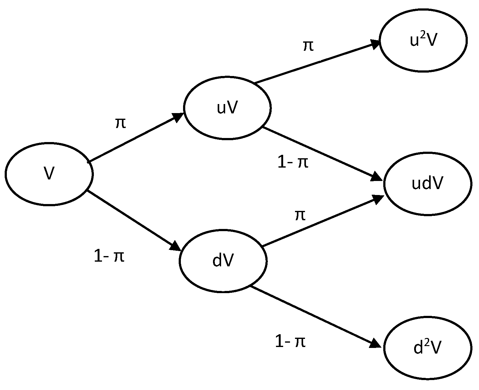
Figure 2.
Option values for flexibility of delaying harvest by 15 years.

Figure 3.
Annual marginal change in option value.
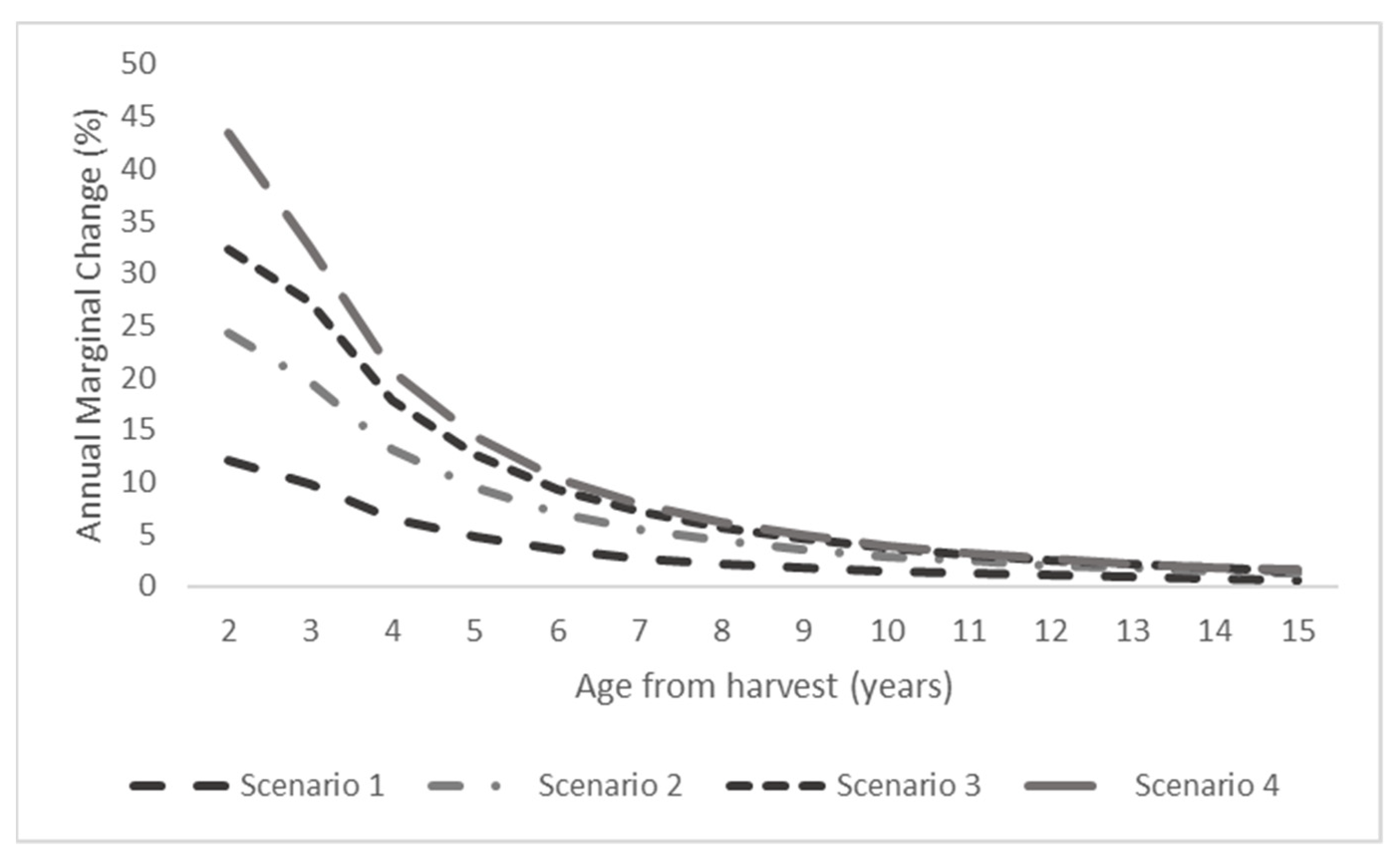
Figure 4.
LEVs based on the Faustmann model, binomial option model and binomial option with carbon payment model.
Figure 4.
LEVs based on the Faustmann model, binomial option model and binomial option with carbon payment model.
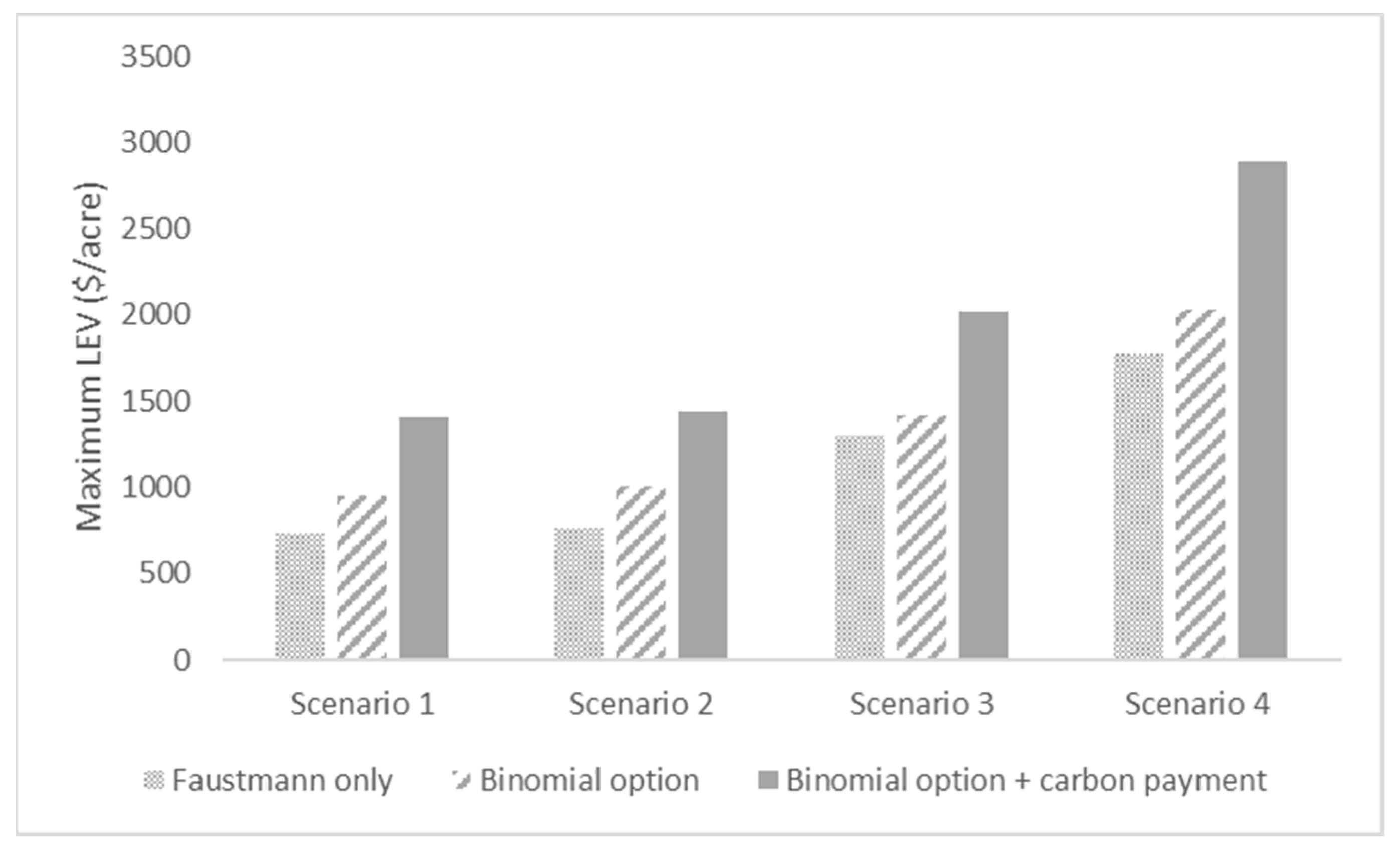
Figure 5.
Optimal rotation age based on the Faustmann model, binomial option model and binomial option with carbon payment model.
Figure 5.
Optimal rotation age based on the Faustmann model, binomial option model and binomial option with carbon payment model.


Table 1.
Scenarios for the study.
| Scenarios | TPA | Management Practices |
|---|---|---|
| Scenario 1 | 400 | No thinning; initial weed control; prescribed fire every 5 years starting age 10 |
| Scenario 2 | 600 | No thinning; initial weed control; prescribed fire every 5 years starting age 10 |
| Scenario 3 | 700 | Artificial regeneration; thinning at age 12, 20; fertilization at age 3, 13, 21; initial weed control only |
| Scenario 4 | 900 | Artificial regeneration; thinning at age 10, 15, 20; fertilization at age 3, 11, 16, 21; initial weed control only |
Table 2.
Summary of costs and revenues associated with managing slash pine.
| Costs/Revenues | Amount | Sources |
|---|---|---|
| Costs | ||
| Site preparation | $158/acre | [52] |
| Planting | $0.1/seedling | |
| Initial weed control | $55/acre | |
| Fertilization at age 3 (Urea only) | $37/acre | |
| Other fertilization (Urea + DAP) | $83/acre | |
| Cruising and marking | $21/acre | |
| Prescribed burning | $30/acre | |
| Annual management costs | $5/acre/year | |
| Annual taxes | $4/acre/year | |
| Aggregator’s fee | 10% of annual total carbon revenue | [32] |
| Verification fee | $0.25/tCO2e/year | |
| Transaction fee | $0.20/tCO2e/year | |
| Revenues | ||
| Sawtimber stumpage price | $31/m3 | [49] |
| Chip-n-saw stumpage price | $24/m3 | |
| Pulpwood stumpage price | $16/m3 | |
| Carbon price | $18/tCO2e | [54] |
Table 3.
Valuation option model parameters.
| Scenario 1 | Scenario 2 | Scenario 3 | Scenario 4 | |
|---|---|---|---|---|
| Investment value | $769 | $823 | $1122 | $1548 |
| Investment cost | $327 | $351 | $329 | $345 |
| Risk-free rate (ρ) | 4% | 4% | 4% | 4% |
| Rotation age (years) | 23 | 24 | 27 | 28 |
| Option time (years) | 15 | 15 | 15 | 15 |
Publisher’s Note: MDPI stays neutral with regard to jurisdictional claims in published maps and institutional affiliations. |
© 2022 by the authors. Licensee MDPI, Basel, Switzerland. This article is an open access article distributed under the terms and conditions of the Creative Commons Attribution (CC BY) license (https://creativecommons.org/licenses/by/4.0/).
Share and Cite
MDPI and ACS Style
Koirala, U.; Adams, D.C.; Susaeta, A.; Akande, E. Value of a Flexible Forest Harvest Decision with Short Period Forest Carbon Offsets: Application of a Binomial Option Model. Forests 2022, 13, 1785. https://doi.org/10.3390/f13111785
AMA Style
Koirala U, Adams DC, Susaeta A, Akande E. Value of a Flexible Forest Harvest Decision with Short Period Forest Carbon Offsets: Application of a Binomial Option Model. Forests. 2022; 13(11):1785. https://doi.org/10.3390/f13111785
Chicago/Turabian StyleKoirala, Unmesh, Damian C. Adams, Andres Susaeta, and Emmanuel Akande. 2022. "Value of a Flexible Forest Harvest Decision with Short Period Forest Carbon Offsets: Application of a Binomial Option Model" Forests 13, no. 11: 1785. https://doi.org/10.3390/f13111785
Note that from the first issue of 2016, this journal uses article numbers instead of page numbers. See further details here.