Forest Aboveground Biomass Estimation in Subtropical Mountain Areas Based on Improved Water Cloud Model and PolSAR Decomposition Using L-Band PolSAR Data

Abstract

Forest aboveground biomass (AGB) retrieval using synthetic aperture radar (SAR) backscatter has received extensive attention. The water cloud model (WCM), because of its simplicity and physical significance, has been one of the most commonly used models for estimating forest AGB using SAR backscatter. Nevertheless, forest AGB estimation using the WCM is usually based on simplified assumptions and empirical fitting, leading to results that tend to overestimate or underestimate. Moreover, the physical connection between the model and the polarimetric synthetic aperture radar (PolSAR) is not established, which leads to the limitation of the inversion scale. In this paper, based on the fully polarimetric SAR data from the Advanced Land Observing Satellite-2 (ALOS-2) Phased Array-type L-band Synthetic Aperture Radar (PALSAR-2), the relative contributions of the three major scattering mechanisms were first analyzed in a hilly area of southern China. On this basis, the traditional WCM was extended by considering the secondary scattering mechanism. Then, to establish the direct relationship between the vegetation scattering mechanism and forest AGB, a new relationship equation between the PolSAR decomposition model and the improved water cloud model (I-WCM) was constructed without the help of external data. Finally, a nonlinear iterative method was used to estimate the forest AGB. The results show that volume scattering is the dominant mechanism, accounting for more than 60%. Double-bounce scattering accounts for the smallest fraction, but still about 10%, which means that the contribution of the double-bounce scattering component is not negligible in forested areas because of the strong penetration capability of the long-wave SAR. The modified method provides a correlation coefficient R² of 0.665 and a root mean square error (RMSE) of 21.902, which is an improvement of 36.42% compared to the traditional fitting method. Moreover, it enables the extraction of forest parameters at the pix scale using PolSAR data without the need for low-resolution external data and is thus helpful for high-resolution mapping of forest AGB.

1. Introduction

Forest aboveground biomass (AGB) is one of the most important parameters for monitoring forest ecosystem [1,2,3]. Therefore, the accurate forest AGB estimation is of great significance for the in-depth study of global carbon balance. The traditional field measurement method is currently the most accurate method for biomass extraction, but the method is labor-intensive, tedious, and destructive, making it difficult to meet the requirements of large-scale mapping. In order to quantify forest AGB from the regional scale to the global scale, different remote sensing technologies, especially space-borne remote sensing, have recently been developed as the primary tools for large-scale forest AGB estimation [4,5]. Optical remote sensing has been used for estimating forest AGB for a relatively long time. However, the applications of optical remote sensing are usually plagued by weather conditions and saturation effects [6,7,8,9]. The use of LiDAR technology for forest parameter estimation has also been reported in much of the literature [10,11,12]. In particular, the new generation of satellite-borne radar, the Ice, Cloud and Land Satellite-2 (ICESat-2), which utilizes the multi-beam micro pulse photon computing technique, has increased the spatial resolution of the spot and has a greater potential for application in the inversion of forest structural parameters [13,14]. However, since its observation range is discrete, it is generally combined with other remote sensing data to meet the needs of large-scale inversion of forest parameters.

SAR systems are of particular interest for estimating and mapping forest AGB because of their relative weather independence and strong penetration. Their penetration depth depends mainly on the wavelength: the longer the wavelength, the deeper the penetration [15,16]. Therefore, long-wavelength SAR systems (L- and P-band) can interact with the main components of forest AGB (i.e., branches and stems), making them more sensitive to forest AGB than short wavelengths (X- and C-band) [17,18,19]. Currently, the SAR techniques used to estimate forest biomass are SAR interferometry (InSAR), polarimetric SAR (PolSAR), polarimetric interferometry (PolInSAR), etc. [20]. Among them, the PolSAR technique uses different polarization states of electromagnetic waves to extract information from different scattering targets. The analysis of PolSAR data sometimes makes it possible to separate the contributions of different scattering mechanisms in a single SAR resolution cell. In forest research, these scattering elements commonly refer to surface scattering, volume scattering, and double-bounce scattering [17]. Compared to InSAR or PolInSAR variables, the variables decomposed by the PolSAR technique have lower saturation for biomass but are widely used as estimation parameters because of their large-scale availability [21]. In addition, because of the specialized side-looking imaging method and strong penetrating characteristics, the advantage of long-wavelength PolSAR for forest parameters depends on canopy moisture, forest structure and topography, etc. [22,23]. Among these, the complex terrain conditions can have an impact on both the azimuthal and distance directions of PolSAR data. Specifically, they mainly include three aspects: polarization orientation angle (POA), effective scattering area (ESA), and angle variation effect (AVE). Therefore, the influence of topography should be considered when inverting forest parameters using PolSAR data in subtropical mountainous areas. In this paper, a fine terrain correction strategy is attempted by considering different polarization channels and different forest cover types on the correction coefficient effects.

At present, there are many models for estimating forest AGB based on PolSAR data, including parametric and non-parametric models [24,25,26]. Among them, the empirical models are generally used to estimate forest AGB by establishing a function between in situ AGB samples and variables derived from SAR data (e.g., backscatter coefficient) [27]. Although it has been reported that the expected results can be achieved using the empirical models in some test areas [28,29], up to now, there is not a consensus on determining an optimal and universal empirical model. In addition, the accuracy of the model parameters fitting mainly depends on the accuracy of the measured data. This means that a large number of field test data of different vegetation types, vertical structures, and growth environment conditions need to be collected for large-scale inversions, which is often difficult [30]. Instead of relying on measured data, the physical models derived based on physical principles are ideal for large-scale estimation [31]. However, the physical models are difficult to use directly for forest AGB estimation because of the need to input large numbers of complex parameters [32]. Therefore, in order to achieve flexibility in applications, the physical models developed for forest parameter retrieval are usually limited in the influencing factors and the types of scattering mechanisms that can be considered. A reasonable compromise between these opposing requirements is to use semi-empirical models. One of the most widely employed semi-empirical models is the water cloud model (WCM) [33]. The backscatter signal is interpreted in terms of direct scattering mechanisms from the ground and the vegetation canopy. Each scattering mechanism is modeled in the original WCM as a straightforward function connected to the structural or biophysical characteristics of the vegetation and ground. The WCM has been frequently utilized to express the correlation between SAR backscatter coefficients and forest AGB for space-borne SAR data at various wavelengths because of its simplicity [33,34].

However, because of the weak ability of shortwave SAR to penetrate vegetation canopy, coupled with the strong attenuation of vegetation canopy and the diffuse scattering from rough ground, when expressing parameters in the WCM, mostly only the single scattering mechanisms (i.e., volume scattering and surface scattering) were considered, and the interaction of SAR signal between ground and tree trunk was ignored [35,36,37]. The absence of the higher-order scattering mechanisms limits the application areas of the WCM at longer wavelengths, for example, over areas with sparse vegetation. Therefore, one of the concerns of this study is to extend the traditional WCM by introducing higher-order scattering to make it more compatible with long wavelength SAR application scenarios. In addition, in order to estimate forest AGB from the WCM, it is necessary to obtain the scattering contribution of different scattering mechanisms in a single pixel of SAR data. One way is to use the single- or dual-polarization SAR data to identify the amount of vegetation scattering and surface scattering in the total backscattering value of a single pixel by setting a canopy cover threshold [33,38,39]. The process of calculating the scattering approximation for different scatters is very complex. Another way is to use the fully polarimetric SAR data to obtain the decomposition components of different scatters within a single-resolution cell, and these decomposition components are obtained using the PolSAR decomposition model [40,41]. However, this approach does not establish a direct link between the decomposition model and the forest AGB, leading to a limited range of applications. Therefore, how to establish a direct link between vegetation scattering mechanisms and forest AGB parameters is another concern of this paper.

To extend the potential of PolSAR for large-scale estimation of forest AGB, we perform terrain correction of the PolSAR data based on the polarization covariance matrix in this study. Then, the semi-empirical WCM is improved by introducing a high-order scattering mechanism, which enhances the stability of the model for characterizing the scattering process of long-wave SAR signal. Third, based on the improved WCM, a pix-scale forest AGB estimation method is proposed, which firstly constructs the relationship equation between the PolSAR decomposition model and the improved WCM based on the topography correction and establishes a direct connection between the vegetation scattering mechanism and forest AGB parameters. Then, a nonlinear iterative method is used to solve the problem of the model parameters estimation at the pixel scale. This method is based on the physical model, which can make the method robust in practical applications.

2. Study Site and Dataset

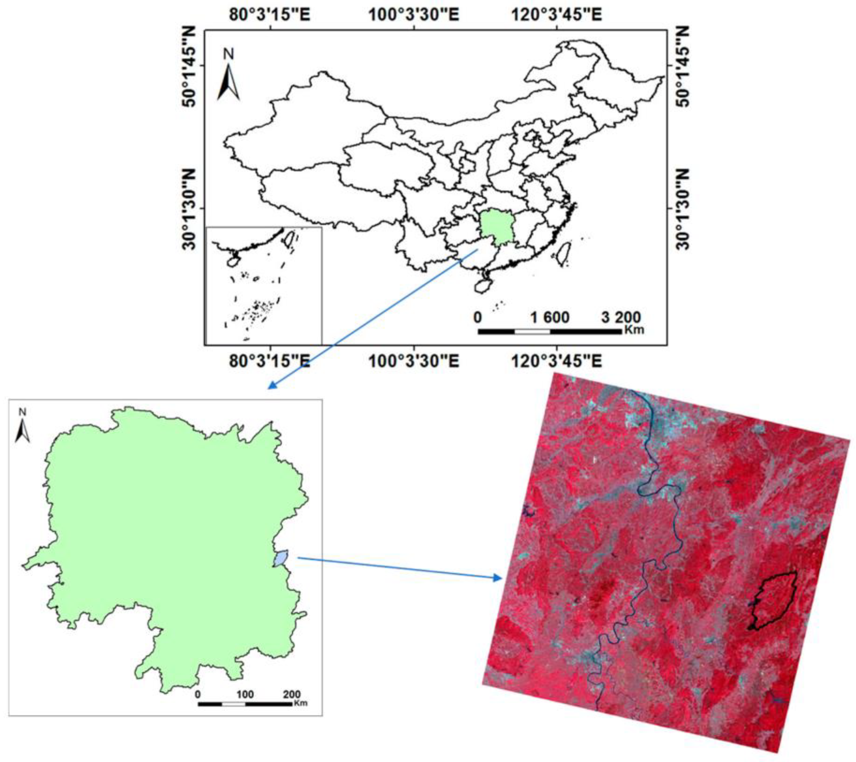
2.1. Study Site

The study area for this work is the Huangfengqiao state-owned forest farm, located in the northeastern of Youxian County, Hunan Province (Figure 1), ranging from 27°05′ to 27°24′ N and 113°35′ to 113°55′ E. It is a field site ground for forest research at Central South University of Forestry and Technology. The ground elevation ranges from 60 m to 1386 m, and the slope ranges from 0 to 84 degrees. This area is located in the subtropical monsoon climate zone, with an annual average temperature of 17.8 °C and an average annual precipitation of 1410.8 mm. The tree species are mainly Chinese fir (Cunninghamia lanceolata), Pinus massoniana Lamb, bamboo, Liriodendron chinense, and Cinnamomum camphora, with the planted Chinese fir being the dominant tree species.

2.2. Ground Data

From June to July 2016, we investigated 60 sample plots with a size of 30 m × 30 m. Each plot, including the central point and corner point, was located using the real-time dynamic measurement global positioning system. In each sample plot, all trees equal to or greater than 5 cm in diameter at breast height (DBH) were measured for their height and DBH. Then, the stem volume of each tree was retrieved as follows [42]:

$$V_i={\displaystyle \sum \pi \times {\left(\frac{1}{2}DB{H}_i\right)}^2\times \left(h_i+3\right)\times f_{\epsilon }}$$

(1)

where $V_i$ represents the stem volume of each tree, $h_i$ denotes the height of ith tree, $\epsilon$ is the tree species, and $f$ is a form factor associated with the tree species [43]. After that, the stem volume of each tree was converted to biomass using the wood density factor, and then, the forest AGB was calculated by combining the number of trees per plot with the following equation [44]:

$$AG{B}_j=n\times V_i\times \rho$$

(2)

where $AG{B}_j$ is the forest aboveground biomass of the jth plot, $n$ is the number of trees within the plot, and $\rho$ denotes the wood density factor of different tree species [45]. After these computations, the total AGB value for individual plots ranged from 2.46 t/ha to 155.52 t/ha, with an average value of 71.67 t/ha. The sample plots were divided into two groups of training samples (n = 44) and validation samples (n = 16) by random sampling. The main parameters of ground-measured plots are provided in

Table 1. Main parameters of ground-measured plots.

Parameter	Range	Mean
DBH (cm)	4.06 to 30.10	17.84
Height (m)	4.60 to 20.20	13.24
Number of stems	30 to 350	96
AGB (t/ha)	2.46 to 155.52	71.67

.

2.3. SAR Data and Ancillary Data

The L-band SAR data over this study area were acquired by the Japanese Aerospace Exploration Agency (JAXA) using the Advanced Land Observing Satellite-2 (ALOS-2) in the polarimetric mode (PLR). The data was acquired along a descending orbit at approximately 4:22 a.m. local time on 14 July 2016. To improve data quality, basic image preprocessing was implemented, including radiometric calibration, multi-look processing (7 × 10), a 7 × 7 Lee filter, and geocoding. The ancillary data mainly include Shuttle Radar Topographic Mission (SRTM) DEM with a resolution of 30 m and a land-use data product. SRTM data were used to assist in geocoding, resampling, and obtaining the angle factor in the terrain correction. The land-use data product was downloaded from the China Geographic State Monitoring Cloud Platform (https://www.dsac.cn/, accessed on 15 August 2023) and was used to assist in terrain correction. According to the secondary land-use classification, forest was subdivided into four types: woodland, shrubbery, spare woodland, and other forest.

3. Method

The main flow of this paper is shown in Figure 2. There are five main steps: (1) basic preprocessing on the original L-band fully polarized SAR data was performed using PolSARpro software (Version 5.1.3, European Space Agency, Paris, France), and the polarization covariance matrix was generated; (2) we carried out topographic correction for the PolSAR data based on the polarization covariance matrix, including POA compensation, ESA correction, and AVE correction; (3) the traditional water cloud model was improved by taking into account the higher-order scattering and the canopy gap; (4) we constructed the relationship between the PolSAR decomposition model and the improved water cloud model and then solved the parameterization by a nonlinear iterative method; (5) the estimation result was verified and compared.

3.1. Polarimetric SAR Terrain Correction

According to the specific influence of terrain on SAR image [46,47], PolSAR data were corrected from three aspects, i.e., POA compensation, ESA correction, and AVE correction based on the polarimetric covariance matrix ($C_3$) [48,49]. The POA compensation was used to reduce the impacts of azimuth slope, as shown in Equation (3):

$$[C_{POA}]=[U_{3(\eta )}][C_3]{[U_{3(\eta )}]}^T$$

(3)

where $C_{POA}$ represents a new rotated polarization covariance matrix and $U_{3(\eta )}$ is a rotation matrix. The shift angle $\eta$ can be estimated by the circular polarization algorithm [44].

The ESA correction for the backscattering coefficient of a single-polarization channel is expressed as follows [46]:

$${\sigma }_{}^0={\beta }_{}^0\times \cos \left(\phi \right)$$

(4)

where $\phi$ is the projection angle, which can be determined by means of DEM and orbit information. $\cos \left(\phi \right)$ is a correction factor of the ESA correction and is used for the polarimetric covariance matrix correction as follows:

$${\left[C_3\right]}_{ESA}=\left[C_3\right]\times \cos \left(\phi \right)$$

(5)

where $C_3$ is the polarimetric covariance matrix after being compensated by POA.

For the single-polarization backscatter coefficient, the simple cosine model proposed by Ulaby is commonly used for AVE correction [50], which can be expressed as

$${\sigma }_{AVE}^0\left({\theta }_{loc}\right)={\sigma }^0\times k\left(n\right), k\left(n\right)={\left(\cos {\theta }_{ref}/\cos {\theta }_{loc}\right)}^n$$

(6)

where ${\theta }_{loc}$ is the local incidence, ${\theta }_{ref}$ is the radar incidence angle, $k\left(n\right)$ is the correction coefficient, and the correction factor n is an unknown parameter. For the PolSAR data, referring to Equation (6), the correction coefficient matrix needs to be constructed, and the equation is given as

$${\left[C_3\right]}_{AVE}={\left[C_3\right]}_{ESA}\mathsf{\Theta }\left[K_i\left(n_{pq}\right)\right]$$

(7)

where $\Theta$ refers to the Hadamard product of two matrices, $i$ is the different types of forest cover, and $p$ and $q$ are incident and scattered wave polarization, respectively. $[K_i(n_{pq})]$ refers to the correction coefficient matrix corresponding to the polarization covariance matrix, which is denoted as

$$\left[K_i(n_{pq})\right]=\left[\begin{array}{ccc}k(n_{hh})& \sqrt{k\left(n_{hh}\right)\cdot k\left(n_{hv}\right)}& \sqrt{k\left(n_{hh}\right)\cdot k\left(n_{vv}\right)}\\ \sqrt{k\left(n_{hh}\right)\cdot k\left(n_{hv}\right)}& k\left(n_{hv}\right)& \sqrt{k\left(n_{hv}\right)\cdot k\left(n_{vv}\right)}\\ \sqrt{k\left(n_{hh}\right)\cdot k\left(n_{vv}\right)}& \sqrt{k\left(n_{hv}\right)\cdot k\left(n_{vv}\right)}& K\left(n_{vv}\right)\end{array}\right]$$

(8)

where $n_{hh}$, $n_{hv}$, and $n_{vv}$ represent the correction factor of HH, HV, and VV polarization channels, respectively.

From Equation (6), the optimal value of n can be obtained by evaluating the minimum correlation between the local incidence angles and the corrected backscatter coefficients. In addition, for the surface covered by vegetation, n represents the change of scattering mechanism caused by the presence of vegetation on the inclined surface [32], which indicates that the value n depends on polarization states and the characteristics of vegetation canopy structure. Thus, we consider the influence of vegetation types and polarization states, which can be expressed as

$$n_{pq}\left(z\right)=\arg \min \left\{\left|\rho \left({\theta }_{loc},{\sigma }_{AVE}^0\left({\theta }_{loc}\right)\right)\right|\right\}$$

(9)

where $\rho$ is the correlation between the local incidence angles and the backscatter coefficients and $n_{pq}$ denotes the optimal correction factor of different polarization. Note that, according to Equation (8), in order to obtain the correction coefficient matrix, we only need to obtain the optimal value of n corresponding to the primary diagonal elements. The results of the optimal n values for different vegetation cover types are shown in

Table 2. The optimal n values for the four vegetation cover types.

Channel	Woodland	Shrubbery	Spare Woodland	Other Forest
HH	1.24	1.23	1.52	1.42
HV	0.82	0.74	0.82	0.63
VV	1.09	1.20	1.39	1.29

.

3.2. AGB Estimation Model

The WCM with gaps in Equation (10) extends the traditional model to consider vertical and horizontal discontinuities in the canopy [51]. In the WCM, the backscatter of a single pixel is contributed by three parts, which are components a, b, and c in Figure 3.

$${\sigma }_{for}^0=(1-\eta ){\sigma }_{gr}^0+\eta {\sigma }_{gr}^0{T}_{tree}+\eta {\sigma }_{veg}^0(1-T_{tree})$$

(10)

where ${\sigma }_{for}^0$ represents the backscatter of a single pixel in the forest area, ${\sigma }_{gr}^0$ is the backscatter coefficient of the ground, ${\sigma }_{veg}^0$ is the direct backscatter coefficient of the forest in the same pixel, the area-fill factor $\eta$ denotes the proportion of vegetation cover in a resolution unit, and $T_{tree}$ is the two-way tree transmissivity.

According to Equation (10), the WCM with gaps is more consistent with the actual situation of forest distribution than the traditional WCM, but the higher-order scattering component is still neglected. After considering the gaps between vegetation layers, the double-bounce scattering component within a resolution cell mainly comes from two possible sources: one is the ground–trunk interaction caused by electromagnetic waves through the vegetation gaps; the other is the ground–trunk interaction caused by electromagnetic waves through the vegetation canopy. The two higher-order scattering contributions can be modeled separately with reference to the modeling method of the original WCM. The total backscatter of the improved water cloud model (IM-WCM) consists of five components, and the expression is as follows:

$${\sigma }_{for}^0=(1-\eta ){\sigma }_{gr}^0+\eta {\sigma }_{gr}^0{T}_{tree}+\eta {\sigma }_{veg}^0(1-T_{tree})+(1-\eta ){\sigma }_{gs}^0+\eta {\sigma }_{gs}^0{T}_{tree}$$

(11)

where ${\sigma }_{gs}^0$ is the backscatter coefficient of the double-bounce scattering, $(1-\eta ){\sigma }_{gs}^0$ represents the double-bounce scattering contribution of the ground–trunk interaction caused by electromagnetic waves through the vegetation gaps, and $\eta {\sigma }_{gs}^0{T}_{tree}$ is the double-bounce scattering of electromagnetic waves after two-way attenuation through the vegetation canopy. Because of the complex distribution of vegetation and gaps, other types of higher-order scattering may exist, such as only one side of the incident and reflected waves being attenuated by the vegetation canopy while the other side does not attenuate. These cases can be regarded as special cases of the double-bounce scattering from ground and trunk interaction and, therefore, can be excluded from the model. For retrieval of the forest AGB, Equation (11) should be expressed as a function related to the forest AGB. Referring to the derivation process of the original WCM [39], Equation (11) can be rewritten as follows:

$${\sigma }_{for}^0={\sigma }_{gr}^0{e}^{-\beta B}+{\sigma }_{veg}^0(1-e^{-\beta B})+{\sigma }_{gs}^0{e}^{-\beta B}$$

(12)

where B represents forest AGB and $\beta$ is the forest transmissivity parameter.

3.3. Model Inversion

The IM-WCM has three scattering contributions to the total forest backscatter of a single pixel. The polarimetric decomposition technique provides the ability to retrieve the three scattering contributions from the PolSAR data, so we rewrite Equation (12) as follows:

$$C_3=C_{3s}{e}^{-\beta B}+C_{3v}(1-e^{-\beta B})+C_{3D}{e}^{-\beta B}$$

(13)

where $C_3$ is the covariance matrix of the total backscatter of the forest and $C_{3s}$, $C_{3v}$, and $C_{3D}$ represent the surface scattering, volume scattering, and double-bounce scattering covariance matrices, respectively. $e^{-\beta B}$ and $(1-e^{-\beta B})$ are the transmissivity terms of the forest. To obtain an estimate of forest AGB from Equation (13), the Freeman component scattering model is used to retrieve different scattering contributions [52].

Based on the surface scattering model, the surface scattering contribution in Equation (13) is defined as follows:

$$w\_c_{3s}=f_{\mathrm{G}}\left[\begin{array}{ccc}1& 0& \alpha \\ 0& 0& 0\\ {\alpha }^{\ast }& 0& {\left|\alpha \right|}^2\end{array}\right]e^{-\beta B},\begin{array}{ccc}\left|\alpha \right|\ge 1& and& \arg (\alpha )\approx 2\varphi \end{array}$$

(14)

where $f_{\mathrm{G}}$ and $\alpha$ represent the contribution of the surface scattering component.

Based on the double-bounce scattering model, the double-bounce scattering contribution in Equation (13) is defined as follows:

$$w\_c_{3\mathrm{D}}=f_{\mathrm{G}}\left[\begin{array}{ccc}1& 0& \alpha \\ 0& 0& 0\\ {\alpha }^{\ast }& 0& {\left|\alpha \right|}^2\end{array}\right]e^{-\beta B},\begin{array}{ccc}\left|\alpha \right|\le 1& and& \arg (\alpha )\approx \pm \pi \end{array}$$

(15)

where $f_{\mathrm{G}}$ and $\alpha$ represent the contribution of the double-bounce scattering component.

Based on the volume scattering model, the volume scattering contribution in Equation (13) is defined as follows:

$$w\_c_{3V}=\frac{f_V}{8}\left[\begin{array}{ccc}3& 0& 1\\ 0& 2& 0\\ 1& 0& 3\end{array}\right]\left(1-e^{-\beta B}\right)$$

(16)

where $f_V$ represents the contribution of the volume scattering component.

By replacing the corresponding scattering contribution term in Equation (13) with Equations (14)–(16), Equation (13) is rewritten as follows:

$$C_3=\left[\begin{array}{ccc}\frac{3}{8}{f}_V(1-e^{-\beta \hspace{0.17em}B})+f_G{e}^{-\beta \hspace{0.17em}B}& 0& \frac{1}{8}{f}_V(1-e^{-\beta \hspace{0.17em}B})+f_G\alpha \hspace{0.17em}{e}^{-\beta \hspace{0.17em}B}\\ 0& \frac{1}{4}{f}_V(1-e^{-\beta \hspace{0.17em}B})& 0\\ \frac{1}{8}{f}_V(1-e^{-\beta \hspace{0.17em}B})+f_G{\alpha }^{*}{e}^{-\beta \hspace{0.17em}B}& 0& \frac{3}{8}{f}_V(1-e^{-\beta \hspace{0.17em}B})+f_G{\left|\alpha \right|}^2{e}^{-\beta \hspace{0.17em}B}\end{array}\right]$$

(17)

According to Equation (17), five independent observations and five equations are provided; i.e., the $C_3$ diagonal provides three, and the C13 term provides two. But, there are six unknown parameters in total, whose vector forms can be expressed as $X=\left\{f_V,f_G,\mathrm{Re}(\alpha ),\mathrm{Im}(\alpha ),\beta ,B\right\}$. Mathematically, the system of equations is underdetermined. However, among the six unknown parameters, the forest transmittance parameter $\beta$ is an empirical coefficient whose value is usually fixed in studies that use WCM to invert forest parameters. In this paper, we first use a nonlinear iterative algorithm to calculate the $\beta$ value of each training sample and take the average value to fix the $\beta$ value. Then, the parameter B is estimated again using the nonlinear iterative algorithm. In the parameter solution process, the results obtained with the traditional Freeman decomposition algorithm are used as the initial values of $f_V$, $f_G$, $\mathrm{Re}\left(\alpha \right)$, and $\mathrm{Im}\left(\alpha \right)$. The initial values of B are determined based on the parameters acquired from the parameterized WCM. The optimization algorithm is the trust domain algorithm, and the parameter boundary conditions are defined as follows:

$$\begin{array}{l}0\le f_V,f_G\le SPAN\\ -4.5\le \mathrm{Re}(\alpha ),\mathrm{Im}(\alpha )\le 4.5\\ 0\le B\le B_{\max }\end{array}$$

(18)

where SPAN is the total power, $\alpha$ boundary reference existing studies [53], and the upper and lower bounds of biomass parameter B refer to the research results of Guo Qinghua’s team [54].

3.4. Model Accuracy Evaluation

The parameterized WCM was utilized to compare with the proposed method in order to assess its inverse accuracy. Equation (12) was parameterized and can be written as follows:

$${\sigma }_{}^0={\beta }_1+{\beta }_2{e}^{\left({\beta }_{3}B\right)}$$

(19)

where ${\beta }_1$, ${\beta }_2$, and ${\beta }_3$ are the unknown parameters of the equation, representing ${\sigma }_{veg}^0$, ${\sigma }_{gr}^0+{\sigma }_{gs}^0-{\sigma }_{veg}^0$, and $-\beta$, respectively. Their values are obtained by fitting the training samples. ${\sigma }_{}^0$, instead of ${\sigma }_{for}^0$, usually refers to the backscatter coefficient for different polarization channels.

In addition, the study used the root mean square error (RMSE) and determinant coefficient (R²) as model evaluation factors to reflect the predictive ability of different models.

4. Results and Analysis

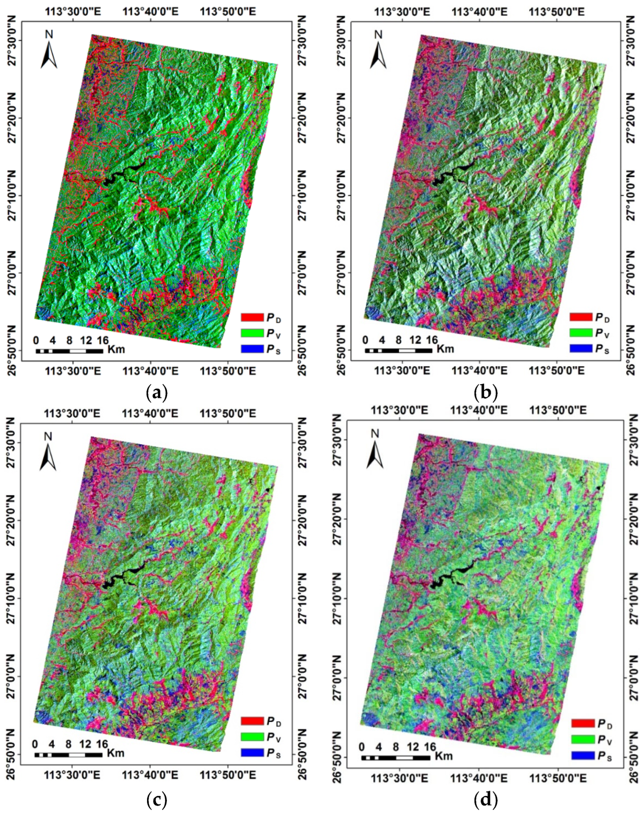
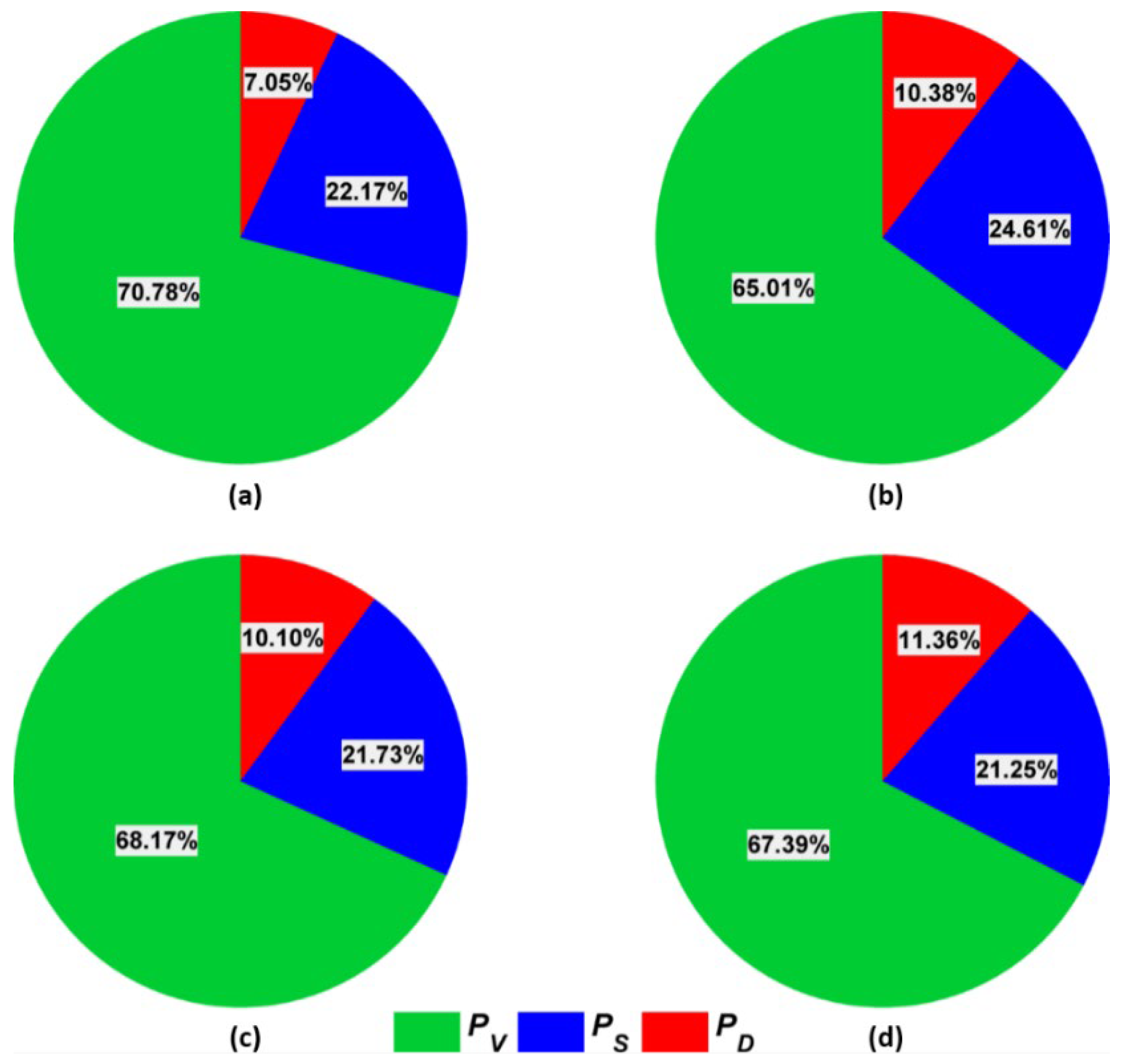
4.1. Effect of Terrain Correction on Scattering Mechanism

In order to evaluate the correction effect of the full polarization SAR data, we analyzed the changes in various polarized scattering mechanisms in the test area. Figure 4 presents the decomposition results from the three-component decomposition after each correction step, where Figure 4a shows the decomposition result of the original data. The different colors represent different decomposition components: the volume scattering component in green, the double scattering component in red, and the surface scattering component in blue.

From the visual perspective of Figure 4, the topographic effect can still be clearly observed after POA compensation (Figure 4b). One of the leading factors is that the influence of the range direction slope is stronger than the azimuth direction for the PolSAR data, while the POA compensation mainly reduces the topographic effect in the azimuth direction. Therefore, this means that the effect of POA compensation on reducing topographic effect is limited. However, compared to the uncompensated case (Figure 4a), it can be seen that the green component of the image in the forest area is reduced. This reflects the inhibition of HV polarization. The ESA correction result is shown in Figure 4b. Obviously, the fluctuation of scattered power with the terrain is improved. However, in areas with more undulating topography, such as ridges, there are still significant topographic effects. The main reason is that these areas usually have large local incidence angles, which require further AVE corrections. In the AVE correction step, the accurate construction of 3D correction coefficient matrix is the key to improving the influence of topography on the scattering mechanism. Substituting the optimal n values in Table 2 into Equation (8), we obtain the correction coefficient matrix for different vegetation types, and the results are shown in

Table 3. The correction coefficient matrices for different vegetation cover types.

Types	K11	K12	K13	K21	K22	K23	K31	K32	K33
Woodland	1.24	2.06	2.35	2.26	0.82	1.91	2.35	1.91	1.09
Shrubbery	1.23	1.97	2.43	1.97	0.74	1.94	2.43	1.94	1.20
Spare woodland	1.52	2.34	2.91	2.34	0.82	2.21	2.91	2.21	1.39
Other forest	1.42	2.05	2.71	2.05	0.63	1.92	2.71	1.92	1.29

K(ij) is the element of the correction coefficient matrices; i and j represent the rows and columns of the element in the matrix, respectively.

. Figure 4d shows the result of AVE correction, which shows that the topographic effect is further removed, and the spatial distribution of the scattered power trend is smooth.

In addition, the color of each image in Figure 4 is different, which may be because terrain correction has different effects on the scattering mechanism of target polarization, primarily by altering the ratio of volume, double, and surface scattering. In this paper, the non-vegetated areas were first masked using the land-use data. Next, using the Freeman–Durden three-component decomposition, surface scattering, volume scattering, and double-bounce scattering mechanisms were obtained. Finally, the scattering power contributions of different scattering mechanisms were counted. The statistical results are shown in Figure 5. After POA compensation (Figure 5b), the proportion of the volume scattering component is 65.01%, the double-bounce scattering component is 10.38%, and the surface scattering component is 24.61%. Compared to POA compensation (Figure 5a), the volume scattering component is reduced by 5.7%, and the double-bounce scattering component increased by 3.33%. This shows that, prior to POA compensation, the volume scattering components are overestimated, and the double-bounce scattering components are underestimated. This phenomenon occurs mainly because the horizontal polarization component received by the radar is no longer parallel to the scattering surface when the radar is imaged on an inclined surface, thus creating excess cross-polarization. Figure 4c shows the percentage of scattering components after ESA correction. Compared to POA compensation, the volume scattering component increases by 3.16%, the surface scattering decreases by 2.88%, and the double-bounce scattering only changes by 0.28%. It is clear that the ESA correction has a greater effect on the volume scattering and surface scattering components, which may depend on the change in the effective scattering area. The AVE correction (Figure 5d) has a smaller effect on the percentage of the volume scattering and surface scattering components, and the double-bounce scattering component has a relatively larger effect, with an increase of 1.26%.

From the overall proportion, the volume scattering component has an absolute advantage in different correction stages, and the proportion is above 60%. The double-bounce scattering component is the smallest among the three components but is still about 10%, which means that the contribution of the double-bounce scattering component is not negligible in forest areas because of the strong penetrating ability of long-wave SAR.

4.2. Forest AGB Estimation

In order to make the system of equations in Equation (17) solvable, the empirical coefficients $\beta$ need to be fixed. The results of $\beta$ value for the training samples is shown in Figure 6. The values of $\beta$ vary mainly within a narrow range between 0.0026 ha/t and 0.0157 ha/t (average of 0.0081 ha/t), with no apparent regional differences. As can be seen from Figure 6, the values $\beta$ may not be the same from one plot to another because the $\beta$ value, as a coefficient of the forest two-way transmittance, is related to vegetation dielectric properties and forest structure, which are often different between individual pixels. Therefore, ideally, the $\beta$ value within the study area may vary per pixel. However, in practice, the lack of detailed meteorological data and forest structure information makes it unrealistic to fine-tune model parameters to accommodate local environmental conditions and forest structure characteristics. This means that under existing conditions, the $\beta$ values are difficult to estimate automatically. In this paper, the $\beta$ value is fixed by taking the average value without considering the influence of external conditions.

After determining the empirical coefficient, the value was substituted into the nonlinear equation system of Equation (17), and the spatial distribution of forest AGB in the test area at the pixel scale could be obtained directly through the nonlinear iterative method. Then, the non-vegetated areas were masked with the help of vegetation cover type data for statistical purposes. Figure 6 presents the ultimate outcomes. The predicted values for the forest AGB range from roughly 0 to 235 t/ha, as shown in Figure 7a, which is a schematic figure for the regional distribution of the forest AGB. The histogram statistics of the estimation findings are shown in Figure 7b. In the test region, the forest AGB has a mean of 69.664 t/ha and a standard deviation of 29.07 t/ha.

According to Equation (19), the parameters of the parameterized WCM usually refer to the backscatter coefficient for different polarization channels. To obtain the optimal backscatter coefficients, we examined the relationship between forest AGB of all sample plots and the polarization channel backscatter using correlation coefficients.

Table 4. Correlation coefficients between AGB and backscatter coefficients.

	HH	HV	VV
Forest AGB	0.395	0.550	0.439

is a list of the outcomes. We discovered that compared to HH or VV, the HV polarization channel exhibited a greater association with the forest AGB. Therefore, the HV backscatter is used as an individual measurement for the parameterized WCM.

The estimation accuracy was verified by validation samples, and the validation results are displayed in Figure 8. The validated plot produced by the conventional nonlinear fitting method has an R² value of 0.384, RMSE of 34.449 t/ha, and RRMSE of 41.398%. For the method proposed in this paper, the correlation coefficient R² value is 0.655, whose RMSE and RRMSE are 21.902 t/ha and 26.321%, respectively. Obviously, the accuracy of the method proposed in this paper is higher than the traditional method, and the accuracy is improved by 15.077%.

5. Discussion

The long-wave SAR backscatter is sensitive to the physical parameters of vegetation and is, therefore, widely used to estimate forest parameters. The water cloud model is one of the most widely used models for estimating forest AGB from SAR backscatter observations because of its ease of use and physical significance. Nevertheless, forest AGB estimation using the WCM is mostly based on simplified assumptions and empirical fitting, leading to results that tend to overestimate or underestimate. One of the underlying assumptions is that higher-order scattering (e.g., double-bounce scattering) can be neglected [33]. In this study, we analyzed the share of three common decomposition components (volume scattering, surface scattering, and double-bounce scattering). Even though it makes up the least amount of the three components, the double-bounce scattering component still contributes roughly 10%, proving that it is not insignificant because of the powerful penetrating power of the long-wave SAR. Therefore, improving the estimation model by introducing the double-bounce scattering can enhance the stability of the model for characterizing the scattering process.

In previous studies, the backscatter contribution of the ground surface and the forest vegetation was obtained as the WCM parameters for the forest AGB inversion using single-polarization or dual-polarization data [55,56]. Estimating the backscatter contribution using single-polarization or dual-polarization SAR data was mathematically rigorous, but the reliability was poor [57,58]. In addition, there were also a few studies based on PolSAR data using polarimetric decomposition techniques to obtain the scattering parameters of the WCM [41]. However, the direct link between decomposition modeling and forest AGB had still not been established. In this study, the Freeman decomposition model was used to create the relationship equation between the scattering model and the improved water cloud model to realize the forest AGB parameter extraction. The volume scattering model in the Freeman decomposition model was performed under the assumption of reflection symmetry. In fact, this symmetry is often observed in forest scattering, especially in planted forests, which is in line with the actual situation of the study area dominated by plantation forests [59]. For some non-uniformly distributed areas of vegetation, such as some natural vegetation with complex trunk and branch shapes and orientations, it is possible that the assumption of reflection symmetry is not met. In this case, other volume scattering models can be considered as the modeling basis [53]. We note that considering the reflection asymmetric case leads to an increase in the number of unknowns in Equation (17). For example, using the volume scattering model in the Yamaguchi four-component decomposition, Equation (17) would have eight unknowns. However, Equation (17) only provides five equations. Therefore, how to balance the number of model unknowns with the number of equations set in the region of non-uniform vegetation structure needs to be further investigated.

The forest transmissivity parameter β in the WCM, which is a parameter related to the vegetation dielectric attributes and forest structure, describes the trend of the backscatter with increasing biomass. Since accurate forest structural information within individual resolution units cannot be obtained, it is difficult to estimate the value of each pixel adaptively. In order to identify plausible ranges of values, the WCM is often initially fitted to the observed relationship of SAR data backscatters and forest biomass using a regression method. Then, a certain value is taken within the value range to fix β [32]. In order to assess the impact of employing a fixed value on retrieval performance, researchers have conducted sensitivity analyses by inverting the model using different values for β and believed that using an average value for biomass retrieval represents a justifiable compromise [33]. In this paper, we draw on this approach. Firstly, the measured forest AGB values of the samples were substituted into the constructed scattering model–water cloud model relationship equation. Then, the nonlinear iterative method was used to estimate the β value. From our results, we can see that the variation range of β value is relatively narrow, and the use of the average value can achieve a better forest AGB estimation result by using a fixed value for β of an average value. It should be noted that since the forest transmissivity depends on the forest structure and the external environment, the average value varies with the study area. For example, in a boreal forest, Santoro et al. found that the variation range of β value was concentrated at 0.004 to 0.008, with a localized range of 0.016 and an average value of 0.006 [38]. In the northeastern United States, Cartus et al. found that the variation range was concentrated at 0.006 to 0.01, with an average value of 0.008 [33]. Therefore, when inverting forest AGB at a larger scale, in order to obtain more desirable estimation results, it can be considered to obtain the range of β value based on different regions or different forest types and then fixed separately. In addition, combining multi-source remote sensing data to obtain forest structure information within the resolution unit and then adaptively estimating the β value at the pixel scale comprise another direction for future effort.

6. Conclusions

In this study, we proposed a method for estimating forest AGB based on an improved water cloud model and polarization decomposition model using L-band PolSAR data in subtropical mountain areas. Prior to the estimation, the polarization covariance matrix was corrected in three steps—POA compensation, ESA correction, and AVE correction—to reduce the influence of complex terrain on PolSAR data in subtropical mountain areas. Then, the relative contributions of the three main scattering mechanisms were analyzed to understand the scattering process of long-wave SAR signals. The results showed that the double-bounce scattering accounted for the smallest but still about 10%, which means that the contribution of the double-bounce scattering component in forested areas is not negligible because of the strong penetration capability of long-wave SAR and the different density distribution structure of the forest. On this basis, in order to establish the direct relationship between the vegetation scattering mechanism and forest AGB, a relationship equation between the PolSAR decomposition model and the improved water cloud model was constructed without the help of external data. Then, a nonlinear iterative method was used to obtain the forest parameters. Compared to the traditional empirical method, the method proposed in this work showed a higher inversion accuracy, with a 36.42% improvement in accuracy. The study explores the ability of the physical model-based inversion of forest AGB at large scales using the long-wave PolSAR technique, and the method has some generality that is helpful and valuable for mapping biomass at large scales.

References

1. Toan, T.L.; Quegan, S.; Davidson, M.W.J.; Balzter, H.; Ulander, L. The BIOMASS mission: Mapping global forest biomass to better understand the terrestrial carbon cycle. Remote Sens. Environ. 2011, 115, 2850–2860. [Google Scholar] [CrossRef]
2. Houghton, R.A.; Hall, F.; Goetz, S.J. Importance of biomass in the global carbon cycle. J. Geophys. Res. 2009, 114, G00E03. [Google Scholar] [CrossRef]
3. Chang, Q.; Zwieback, S.; Devries, B.; Berg, A. Application of L-band SAR for mapping tundra shrub biomass, leaf area index, and rainfall interception. Remote Sens. Environ. 2022, 268, 112747. [Google Scholar] [CrossRef]
4. Huy, B.; Truong, N.Q.; Khiem, N.Q.; Poudel, K.P.; Temesgen, H. Deep learning models for improved reliability of tree aboveground biomass prediction in the tropical evergreen broadleaf forests. For. Ecol. Manag. 2022, 508, 120031. [Google Scholar] [CrossRef]
5. Puliti, S.; Hauglin, M.; Breidenbach, J.; Montesano, P.M.; Astrup, R. Modeling above-ground biomass stock over Norway using national forest inventory data with ArcticDEM and Sentinel-2 data. Remote Sens. Environ. 2020, 236, 111501. [Google Scholar] [CrossRef]
6. Chopping, M.; Wang, Z.; Schaaf, C.; Bull, M.A.; Duchesne, R.R. Forest aboveground biomass in the southwestern United States from a MISR multi-angle index, 2000–2015. Remote Sens. Env. 2022, 275, 112964. [Google Scholar] [CrossRef]
7. Chen, C.; Ma, Y.; Ren, G.B.; Wang, J.B. Aboveground biomass of salt-marsh vegetation in coastal wetlands: Sample expansion of in situ hyperspectral and sentinel-2 data using a generative adversarial network. Remote Sens. Environ. 2022, 270, 112885. [Google Scholar] [CrossRef]
8. Liao, Z.M.; Dijk, A.I.J.M.V.; He, B.B.; Larraondo, P.R.; Scarth, P.F. Woody vegetation cover, height and biomass at 25-m resolution across Australia derived from multiple site, airborne and satellite observations. Int. J. Appl. Earth Obs. 2020, 93, 102209. [Google Scholar] [CrossRef]
9. Fang, P.; Yan, N.N.; Wei, P.P.; Zhao, Y.F.; Zhang, X.W. Aboveground Biomass Mapping of Crops Supported by Improved CASA Model and Sentinel-2 Multispectral Imagery. Remote Sens. 2021, 13, 2755. [Google Scholar] [CrossRef]
10. Beyene, S.M.; Hussin, Y.A.; Kloosterman, H.E.; Ismail, M.H. Forest Inventory and Aboveground Biomass Estimation with Terrestrial LiDAR in the Tropical Forest of Malaysia. Can. J. Remote Sens. 2020, 46, 130–145. [Google Scholar] [CrossRef]
11. Musthafa, M.; Singh, G. Forest above-ground woody biomass estimation using multi-temporal space-borne LiDAR data in a managed forest at Haldwani, India. Adv. Space Res. 2022, 69, 3245–3257. [Google Scholar] [CrossRef]
12. Xu, D.D.; Wang, H.B.; Xu, W.X.; Luan, Z.Q.; Xu, X. LiDAR Applications to Estimate Forest Biomass at Individual Tree Scale: Opportunities, Challenges and Future Perspectives. Forests 2021, 12, 550. [Google Scholar] [CrossRef]
13. Narine, L.L.; Popescu, S.; Neuenschwander, A.; Zhou, T.; Srinivasan, S.; Harbeck, K. Estimating aboveground biomass and forest canopy cover with simulated ICESat-2 data. Remote Sens. Environ. 2019, 224, 1–11. [Google Scholar] [CrossRef]
14. Narine, L.L.; Popescu, S.C.; Malambo, L. Using ICESat-2 to estimate and map forest above ground biomass: A First Example. Remote Sens. 2020, 12, 1824. [Google Scholar] [CrossRef]
15. Englhart, S.; Keuck, V.; Siegert, F. Aboveground biomass retrieval in tropical forests-The potential of combined X- and L- band SAR data use. Remote Sens. Environ. 2011, 115, 1260–1271. [Google Scholar] [CrossRef]
16. Carreiras, J.M.B.; Quegan, S.; Le Toan, T.; Dinh, H.T.M.; Saatchi, S.S.; Carvalhais, N.; Reichstein, M.; Scipal, K. Coverage of high biomass forests by the ESA BIOMASS mission under defense restrictions. Remote Sens. Environ. 2017, 196, 154–162. [Google Scholar] [CrossRef]
17. Santoro, M.; Cartus, O. Research Pathways of Forest Above-Ground Biomass Estimation Based on SAR Backscatter and Interferometric SAR Observations. Remote Sens. 2018, 10, 608. [Google Scholar] [CrossRef]
18. Cartus, O.; Santoro, M.; Wegmueller, U.; Rommen, B. Benchmarking the retrieval of biomass in boreal forests using P-band SAR backscatter with multi-temporal C-and L-band observations. Remote Sens. 2019, 11, 1695. [Google Scholar] [CrossRef]
19. Pardini, M.; Cazcarra-Bes, V.; Papathanassiou, K.P. TomoSAR Mapping of 3D Forest Structure: Contributions of L-Band Configurations. Remote Sens. 2021, 13, 2255. [Google Scholar] [CrossRef]
20. Fu, B.; Xie, S.; He, H.; Zuo, P.; Sun, J.; Liu, L.; Huang, L.; Fan, D.; Gao, E. Synergy of multi-temporal polarimetric SAR and optical image satellite for mapping of marsh vegetation using object-based random forest algorithm. Ecol. Indic. 2021, 131, 108173. [Google Scholar] [CrossRef]
21. Lucas, R.; Armston, J.; Fairfax, R.; Fensham, R.; Accad, A.; Carreiras, J.; Kelley, J.; Bunting, P.; Clewley, D.; Bray, S.; et al. An Evaluation of the ALOS PALSAR L-Band Backscatter—Above Ground Biomass Relationship Queensland, Australia: Impacts of Surface Moisture Condition and Vegetation Structure. IEEE J. Sel. Top. Appl. Earth Observ. Remote Sen. 2010, 3, 576–593. [Google Scholar] [CrossRef]
22. Zhang, H.B.; Zhu, J.J.; Wang, C.C.; Lin, H.; Liu, Z.W. Forest Growing Stock Volume Estimation in Subtropical Mountain Areas Using PALSAR-2 L-Band PolSAR Data. Forests 2019, 10, 276. [Google Scholar] [CrossRef]
23. Mermoz, S.; Le Toan, T.; Villard, L.; Réjou-Méchain, M.; Seifert-Granzin, J. Biomass assessment in the Cameroon savanna using ALOS PALSAR data. Remote Sens. Environ. 2014, 155, 109–119. [Google Scholar] [CrossRef]
24. Carreiras, J.M.B.; Vasconcelos, M.J.; Lucas, R.M. Understanding the relationship between aboveground biomass and ALOS PALSAR data in the forests of GuineaBissau (West Africa). Remote Sens. Environ. 2012, 121, 426–442. [Google Scholar] [CrossRef]
25. Michelakis, D.; Stuart, N.; Brolly, M.; Woodhouse, I.H.; Lopez, G.; Linares, V. Estimation of woody biomass of pine savanna woodlands from ALOS PALSAR images. IEEE J. Sel. Top. Appl. Earth Observ. Remote Sens. 2015, 8, 244–254. [Google Scholar] [CrossRef]
26. Schlund, M.; Scipal, K.; Quegan, S. Assessment of a Power Law Relationship between P-Band SAR Backscatter and Aboveground Biomass and Its Implications for BIOMASS Mission Performance. IEEE J. Sel. Top. Appl. Earth Observ. Remote Sens. 2018, 11, 3538–3547. [Google Scholar] [CrossRef]
27. Peregon, A.; Yamagata, Y. The use of ALOS/PALSAR backscatter to estimate above-ground forest biomass: A case study in Western Siberia. Remote Sens. Environ. 2013, 137, 139–146. [Google Scholar] [CrossRef]
28. Hame, T.; Ahola, H.; Antropov, O.; Rauste, Y. Stand-Level Stem Volume of Boreal Forests from Spaceborne SAR Imagery at L-Band. IEEE J. Sel. Top. Appl. Earth Obs. Remote Sens. 2013, 6, 35–44. [Google Scholar]
29. Long, J.P.; Lin, H.; Wang, G.X.; Sun, H.; Yan, E.P. Mapping growing stem volume of Chinese Fir Plantation using a saturation-based multivariate method and quad-polarimetric SAR images. Remote Sens. 2019, 11, 1872. [Google Scholar] [CrossRef]
30. Santoro, M.; Cartus, O.; Fransson, J.E.S. Integration of allometric equations in the water cloud model towards an improved retrieval of forest stem volume with L-band SAR data in Sweden. Remote Sens. Environ. 2021, 253, 112235. [Google Scholar] [CrossRef]
31. Lu, D.S.; Chen, Q.; Wang, G.X.; Liu, L.J.; Li, G.Y.; Moran, E. A survey of remote sensing-based aboveground biomass estimation methods in forest ecosystems. Int. J. Digit. Earth 2016, 9, 63–105. [Google Scholar] [CrossRef]
32. Santoro, M.; Beaudoin, A.; Beer, C.; Fransson, J.E.S.; Hall, R.J.; Pathe, C.; Schmullius, C.; Schepaschenko, D.; Shvidenko, A. Forest growing stock volume of the northern hemisphere: Spatially explicit estimates for 2010 derived from Envisat ASAR. Remote Sens. Env. 2015, 168, 316–334. [Google Scholar] [CrossRef]
33. Cartus, O.; Santoro, M.; Kellndorfer, J. Mapping forest aboveground biomass in the Northeastern United States with ALOS PALSAR dual-polarization L-band. Remote Sens. Environ. 2012, 124, 446–478. [Google Scholar] [CrossRef]
34. Santoro, M.; Cartus, O.; Fransson, J.E.S.; Wegmüller, U. Complementarity of X-, C-, and L-band SAR Backscatter Observations to Retrieve Forest Stem Volume in Boreal Forest. Remote Sens. 2019, 11, 1563. [Google Scholar] [CrossRef]
35. Dobson, M.C.; Ulaby, F.T.; Le Toan, T.; Beaudoin, A.; Christensen, N. Dependence of radar backscatter on coniferous forest biomass. IEEE Trans. Geosci. Remote Sens. 1992, 30, 412–415. [Google Scholar] [CrossRef]
36. Pulliainen, J.T.; Kurvonen, L.; Hallikainen, M.T. Multitemporal behavior of L- and C-band SAR observations of boreal forests. IEEE Trans. Geosci. Remote Sens. 1999, 37, 927–937. [Google Scholar] [CrossRef]
37. Ningthoujam, R.K.; Balzter, H.; Tansey, K.; Feldpausch, T.R.; Mitchard, E.T.A.; Wani, A.A.; Joshi, P.K. Relationships of S-band radar backscatter and forest aboveground biomass in different forest types. Remote Sens. 2017, 9, 1116. [Google Scholar] [CrossRef]
38. Santoro, M.; Beer, C.; Cartus, O.; Schmullius, C.; Shvidenko, A.; McCallum, I.; Wegmüller, U.; Wiesmann, A. Retrieval of growing stock volume in boreal forest using hyper-temporal series of Envisat ASAR ScanSAR backscatter measurements. Remote Sens. Environ. 2011, 115, 490–507. [Google Scholar] [CrossRef]
39. Bouvet, A.; Mermoz, S.; Le Toan, T.; Villard, L.; Mathieu, R.; Naidoo, L.; Asner, G.P. An above-ground biomass map of African savannahs and woodlands at 25 m resolution derived from ALOS PALSAR. Remote Sens. Environ. 2018, 206, 156–173. [Google Scholar] [CrossRef]
40. Bharadwaj, P.S.; Kumar, S.; Kushwaha, S.; Bijker, W. Polarimetric scattering model for estimation of above ground biomass of multilayer vegetation using ALOS-PALSAR quad-pol data. Phys. Chem. Earth 2015, 83, 187–195. [Google Scholar] [CrossRef]
41. Kumar, S.; Garg, R.D.; Govil, H.; Kushwaha, S. PolSAR-Decomposition-Based Extended Water Cloud Modeling for Forest Aboveground Biomass Estimation. Remote Sens. 2019, 11, 2287. [Google Scholar] [CrossRef]
42. Deng, S.Q.; Katoh, M.; Guan, Q.W.; Yin, N.; Li, M.Y. Estimating forest aboveground biomass by combining ALOSPALSAR and Word View-2 data: A case study at purple mountain national park, Nanjing, China. Remote Sens. 2014, 6, 7878–7910. [Google Scholar] [CrossRef]
43. Zhang, X.Q.; Zhang, J.G.; Duan, A.G. Compatibility of Stand Volume Model for Chinese Fir Based on Tree-Level Stand-Level. Sci. Silvae Sin. 2014, 50, 83–87. [Google Scholar]
44. Ghasemi, N.; Tolpekin, V.; Stein, A. Assessment of Forest Above-ground Biomass Estimation from PolInSAR in The Presence of Temporal Decorrelation. Remote Sens. 2018, 10, 815–837. [Google Scholar] [CrossRef]
45. Pereira, L.O.; Furtado, L.F.A.; Novo, E.M.L.M.; Sant’Anna, S.J.S.; Liesenberg, V.; Silva, T.S.F. Multifrequency and full-polarimetric SAR assessment for estimating above ground biomass and leaf area index in the Amazon Várzea wetlands. Remote Sens. 2018, 10, 1355. [Google Scholar] [CrossRef]
46. Lee, J.S.; Schuler, D.L.; Ainsworth, T.L. Polarimetric SAR data compensation for terrain azimuth slope variation. IEEE Trans. Geosci. Remote Sens. 2000, 38, 2153–2163. [Google Scholar]
47. Zhao, L.; Chen, E.X.; Li, Z.Y.; Zhang, W.F.; Gu, X.Z. Three-Step Semi-Empirical Radiometric Terrain Correction Approach for PolSAR Data Applied to Forested Areas. Remote Sens. 2017, 9, 269. [Google Scholar] [CrossRef]
48. Small, D. Flattening gamma: Radiometric terrain correction for SAR imagery. IEEE Trans. Geosci. Remote Sens. 2011, 49, 3081–3093. [Google Scholar] [CrossRef]
49. Castel, T.; Beaudoin, A.; Stach, N.; Stussi, N.; Le Toan, T.; Durand, P. Sensitivity of space-borne SAR data to forest parameters over sloping terrain. Theory and experiment. Int. J. Remote Sens. 2001, 22, 2351–2376. [Google Scholar] [CrossRef]
50. Ulaby, F.T.; Moore, R.K.; Fung, A.K. Volume Scattering and Emission Theory. In Microwave Remote Sensing Active and Passive; Artech House: Norwood, MA, USA, 1982; Volume III. [Google Scholar]
51. Askne, J.I.H.; Dammert, P.B.G.; Ulander, L.M.H. C-band repeat-pass interferometric SAR observations of the forest. IEEE Trans. Geosci. Remote Sens. 1997, 35, 25–35. [Google Scholar] [CrossRef]
52. Freeman, A. Fitting a tow-component scattering model to polarimetric SAR data from forests. IEEE Trans. Geosci. Remote Sens. 2007, 45, 2583–2592. [Google Scholar] [CrossRef]
53. Xie, Q.H.; Berman, J.D.B.; Lopez-sanchez, J.M.; Zhu, J.J.; Wang, C.C. Quantitative analysis of polarimetric model-based decomposition methods. Remote Sens. 2016, 8, 977. [Google Scholar] [CrossRef]
54. Su, Y.J.; Guo, Q.H.; Xue, B.L.; Hu, T.Y.; Alvarez, O.; Tao, S.L.; Fang, J.Y. Spatial distribution of forest aboveground biomass in China: Estimation through combination of spaceborne lidar, optical imagery, and forest inventory data. Remote Sens. Environ. 2016, 173, 187–199. [Google Scholar] [CrossRef]
55. Huang, X.; Ziniti, B.; Torbick, N.; Ducey, M.J. Assessment of forest above ground biomass estimation using multi-temporal C-band Sentinel-1 and Polarimetric L-band PALSAR-2 data. Remote Sens. 2018, 10, 1424. [Google Scholar] [CrossRef]
56. Santoro, M.; Wegmüller, U.; Askne, J. Forest stem volume estimation using C-band interferometric SAR coherence data of the ERS-1 mission 3-days repeat-interval phase. Remote Sens. Environ. 2018, 216, 684–696. [Google Scholar] [CrossRef]
57. Ranson, K.J.; Sun, G.; Weishampel, J.F.; Knox, R.G. Forest biomass from combined ecosystem and radar backscatter modeling. Remote Sens. Environ. 1997, 59, 118–133. [Google Scholar] [CrossRef]
58. Kumar, S.; Pandey, U.; Kushwaha, S.P.; Chatterjee, R.S.; Bijker, W. Aboveground biomass estimation of tropical forest from Envisat advanced synthetic aperture radar data using modeling approach. J. Appl. Remote Sens. 2012, 6, 063588. [Google Scholar] [CrossRef]
59. Souyris, J.C.; Imbo, P.; Fjortoft, R.; Mingot, S.; Lee, J.S. Compact polarimetry based on symmetry properties of geophysical media: The π/4 mode. IEEE Trans. Geosci. Remote Sens. 2005, 43, 634–646. [Google Scholar] [CrossRef]
Figure 1. Study area and the corresponding polarimetric RGB image.
Forests 14 02303 g001
Figure 2. The main flow of this paper.
Forests 14 02303 g002
Figure 3. The total backscattering composition of the IM-WCM; a is the backscatter from the canopy, b is the ground backscatter attenuated by the canopy; c is the direct ground backscatter through gaps in the vegetation; d is the double-bounce scattering through gaps in the vegetation; e is the double-bounce scattering attenuated by the canopy.
Forests 14 02303 g003
Figure 4. PolSAR decomposition results with different terrain correction steps: (a) Original data; (b) POA compensation; (c) ESA correction; (d) AVE correction. The colors of the images are PD (red), PV (green), and PS (blue). PD, PV, and PS are the powers of the double scattering, volume scattering, and surface scattering mechanisms, respectively.
Forests 14 02303 g004
Figure 5. Scattering component power statistics: (a) Original data; (b) after POA compensation; (c) after ESA correction; (d) after AVE correction. Pv: volume scattering power, Ps: surface scattering power, Pd: double-bounce scattering power.
Forests 14 02303 g005
Figure 6. Distribution of empirical coefficient β.
Forests 14 02303 g006
Figure 7. Results of Forest AGB estimation in the study region: (a) forest AGB spatial distribution; (b) histogram of AGB map.
Forests 14 02303 g007
Figure 8. The relationship between predicated forest AGB and reference forest AGB using test sample dataset: (a) The method proposed in this paper; (b) the parameterized WCM.
Forests 14 02303 g008