
Elastoplastic Analysis of Timber Connections with Dowel-Type Fasteners at Ambient and High Temperatures

1
Graduate School of Science and Engineering, Chiba University, 1-33, Yayoi-cho, Inage-ku, Chiba-shi 263-8522, Chiba, Japan
2
Department of Architecture, Graduate School of Engineering, 1-33, Yayoi-cho, Inage-ku, Chiba-shi 263-8522, Chiba, Japan
*
Author to whom correspondence should be addressed.
Forests 2023, 14(2), 373; https://doi.org/10.3390/f14020373
Submission received: 16 January 2023
/
Revised: 8 February 2023
/
Accepted: 8 February 2023
/
Published: 12 February 2023
(This article belongs to the Section Wood Science and Forest Products)
Abstract
:Three-dimensional elastoplastic finite element (FE) analysis models considering a damage zone and cleavage were developed, including plastic behavior of embedment tests parallel and perpendicular to the grain at ambient and high temperatures, in order to study the embedment behavior of timber. In a numerical analysis of compression tests to define material properties of timber, the post-yield behavior of the X-axis in the axial direction was larger than the test values when the post-yield slope of the test result were set to the plastic modulus. The reason was that the stress on the Y-axis and Z-axis increased after the yield point; thus, the equivalent yield stress decreased. In the numerical analysis of the embedment tests, the effect of the damage zone must be considered in the analytical models because the initial stiffness of the numerical results in compression parallel to the grain was considerably higher than that of the test results when the damage zone was not considered. In the numerical analysis of the embedment tests in compression perpendicular to the grain, the two models reproduced the stiffness and behavior after the yield point of the test results. The model that considered cleaving showed the stress distribution after cleavage.
1. Introduction
In recent years, the demand for timbers for medium- and large-scale structures around the world has increased for environmental reasons. Connections are often one of the weak points of timber structures and determine their load-carrying capacity [1]. In addition, fire resistance must be ensured for medium- and large-scale structures. Therefore, a better understanding of the mechanical behavior of connections is important for structural design, including fire safety design of medium- and large-scale timber structures.
Dowel-type connections, such as bolts or dowels with steel plates, are common timber-to-timber connections. The mechanical behavior of these types of connections has been investigated at room temperature in many previous experimental studies (e.g., [2,3,4,5]), and the European Yield Model [6] is used in the current design codes (Eurocode 1995-EC5) for timber structures [7]. However, there is a discrepancy between the failure modes observed in experiments and those predicted by design codes [8]. To develop new connections, experimental or numerical results are important. The connections used in actual buildings vary in terms of fiber direction, timber thickness, and number and arrangement of dowels. Therefore, the previous experimental studies are not sufficient for the design of timber connections.
The elastoplastic FE analysis is useful to analyze the behavior of different connections. However, an analytical model has not been fully established. The main problem that complicates the prediction of the behavior of timber connections is the anisotropy of timber and the description of the constitutive law of timber. Oudjene et al. [9] presented a 2D FE model for compression tests and 3D FE model for embedment tests parallel and perpendicular to the grains at ambient temperature focusing on a plastic behavior. The analysis results including yield point, plastic stiffness, and plasticity hardening successfully compared with test results. In addition, Xu. Et al. [10] studied the behavior of a dowel-type connection with steel-to-timber-loaded tension perpendicular to the grain at ambient temperature using FE analysis. The analysis results demonstrated good agreement between experimental values and initial stiffness and yield point.
There are many types of connections in timber structures, and their design requires a large amount of test data. In addition, large-scale tests under fire conditions are very expensive. FE analysis is an effective method for investigating the fire behavior of timber connections because the complex behavior is influenced by several parameters, such as the fiber direction, timber thickness, number and arrangement of dowels, and the different thermophysical and thermomechanical properties of these materials. While steel dowels can maintain almost the same strength at high temperatures up to 300 °C as at ambient temperature, the strength of timber at 100 °C drops to less than half of the strength at ambient temperature [7]. Therefore, it is particularly important to understand the embedment behavior of timber connections at high temperatures, and experimental studies have been conducted [11,12,13,14]. Cachim et al. [15] proposed a numerical method using spring models for timber connections with dowel compression parallel and perpendicular to the grain at high temperatures. Nakayama et al. [16] developed a numerical model for non-linear M-θ relationships under fire conditions (non-linear M-θ model) that considers the temperature and plasticization of dowels and timber. Audebert et al. [17] and Khelifa et al. [18] performed 3D FE analyzes for dowel-type timber connections loaded in tension perpendicular to the grain at high temperatures. However, most previous studies using FE analysis for timber connections were performed only at ambient temperatures or up to the elastic range.
Therefore, this study presents 3D elastoplastic FE models of compression and embedment tests (including plastic behavior) with timber parallel or perpendicular to the grain at ambient and high temperatures. In particular, we focused on the complex behavior around the connections at the yield points and the plastic range at ambient and high temperatures. We also developed a modeling method for FE analysis of embedment tests, which is important for this study.
2. Materials and Methods
Calibrating material properties (Young’s modulus and yield stress) is supposed to be able to accurately reproduce embedment test results. Therefore, this study consists of FE analysis of compression and embedment tests.
2.1. Compression Tests
Before conducting embedment tests of the dowel connection, it is necessary to understand the mechanical properties of compression of glulam at ambient and high temperatures.
2.1.1. Materials and Methods of Compression Tests
Kawarabayashi et al. conducted compression tests parallel and perpendicular to the gain using the structural glulam made of Japanese cedar (Cryptomeria japonica) and Japanese larch (Larix kaempferi) [13]. We use this data and provide a brief overview of the test in this section. This test was performed the method that is based on the standards [19]. Figure 1 shows the test information of compression tests. The specimen was 300 mm (high) × 75 mm (wide) × 75 mm (deep) and consisted of three 25 mm-thick laminae (compression parallel to the grain) or ten 30 mm-thick laminae (compression perpendicular to the grain).
The heating conditions are listed in Table 1. The values under “heating time” in Table 1 indicate number of specimens. The test parameters were heating temperature (60 °C, 100 °C, 150 °C, 200 °C), heating times, and fiber directions. A hot air generator was used to heat the specimens, which could heat up to 200 °C and keep the temperature constant. Figure 2 shows the arrangement of temperature measurements. The temperature was measured at two points: the center (37.5 mm from the edge) and edge (9.4 mm from the edge). The measured temperature values are listed in Table 2 (from a previous study [12]). A 1 MN Amsler compression tester was used for loading, and the load was applied until the specimen fractured. For the load measurement, a load cell was used at the bottom of the specimen, and the relative displacement was measured with a compressometer over a length of 150 mm.
The red bullets in the Figure 2 indicate locations of temperature measurement.
2.1.2. Bilinearization of Stress–Strain Relationship from the Test Results
From the test results, the stress was obtained by dividing the load by the cross-sectional area (75 × 75 mm), and the strain was obtained by dividing the relative displacement by the measurement section (150 mm). Because the FE analysis requires the stress–strain relationship using a bilinear model, the Young’s modulus (E1), plastic modulus, and yield point (εy, σy) were determined from the test results. The method for determining the Young’s modulus and yield point is shown in Figure 3. The Young’s modulus (E1) was determined using Equation (1).
where
- σmax0.5: 50 % stress of the maximum stress;
- σmax0.1: 10 % stress of the maximum stress;
- εn: strain at σmax0.5
- εi: strain at σmax0.1.
Figure 3.
Determination method of Young’s modulus and yield point. (a) Compression parallel to the grain; (b) compression perpendicular to the grain.
Figure 3.
Determination method of Young’s modulus and yield point. (a) Compression parallel to the grain; (b) compression perpendicular to the grain.
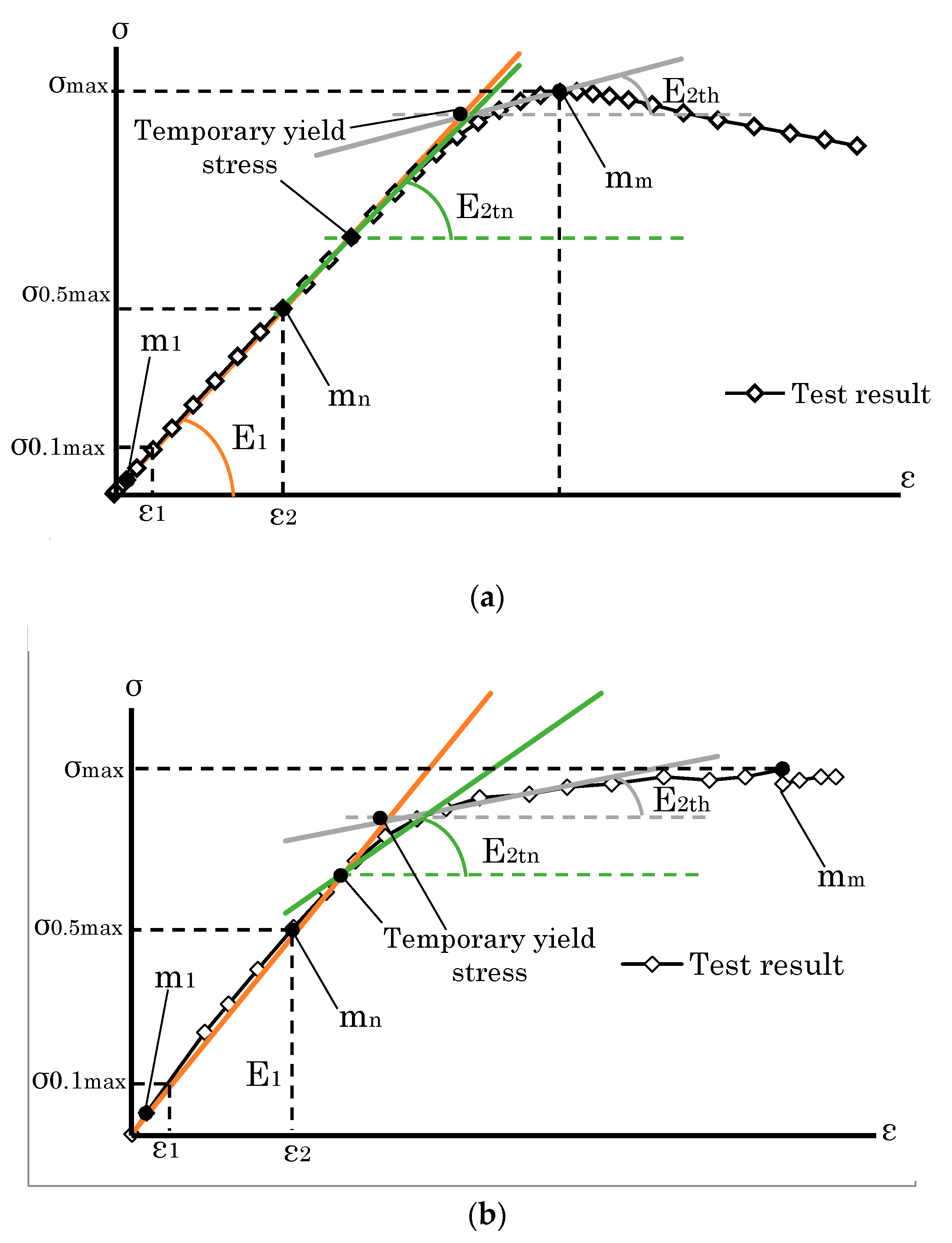
The intersection point of Young’s modulus and plastic modulus defines the yield point. Therefore, the yield point depends on the plastic modulus. A flowchart for determining the yield point is shown in Figure 4. The yield stress was calculated with reference to a method of Inayama [20]. The letters in the flowchart correspond to Figure 3 and Equations (2)–(8). The flowchart consists of a step in Figure 3 that creates an approximate line (inside the green box in Figure 4) and another step in Figure 3 that finds the approximate line created in Step 1 that best matches the test values (inside the orange box in Figure 4). The temporary plastic modulus and temporary yield point were calculated using the test data from point mn(εn,σ0.5max) to point mm(εm,σmax), and the yield point was determined using the test results from point m1 to point mm. The starting point was taken from mn to mm−4 (=h), and an approximate line was made at five points from the starting point. For example, the green line in Figure 3 is the approximate line calculated at five points (mn,mn+1,mn+2,mn+3,mn+4) with mn as the starting point. The slope of the approximate line at the starting point mh is defined as the temporary plastic modulus (E2th), and the intersection with Young’s modulus is defined as the temporary yield point (εyth,σyth). As shown in Equation (8), the yield point is the temporary yield point determined by h when the sum of the squared difference between the test value and calculated stresses (e.g., σanalk in Figure 5) from m1 to mm is minimized, as shown in Figure 5. The temporary plastic modulus is the plastic modulus at which the yield point is determined. The calculated stresses (e.g., σanalk in Figure 5) can be determined using the Young’s modulus in the elastic range or the temporary plastic modulus and temporary yield stress in the plastic range. Table 3 lists the determined Young’s modulus and yield stress.
- σj: Stress from the test result at point j;
- εj: Strain from the test result at point j;
- aa is E1 when εj is less than εyth and Et2h when εj is greater than εyth;
- bb is 0 when εj is less than εyth and bh when εj is greater than εyth.
2.1.3. Material Properties at High Temperature Used in FE Analysis
The reduction factors of the yield strength and Young’s modulus at high temperature were determined under the following six assumptions:
First assumption: Ambient temperature was room temperature during compression tests (cedar: 12 °C, larch: 23 °C).
Second assumption: The charring temperature was set at 300 °C, and the reduction factor of yield strength or Young’s modulus at 300 °C was zero according to Eurocode5 [7].
Third assumption: To determine the yield strength and Young’s modulus at high temperature from the test results, the average temperature of the test value at two points was used as the timber temperature. In other words, the temperature distribution was assumed to be linear because the heating rate was relatively slow during the test. The average temperature is referred to as the overall temperature of the timber.
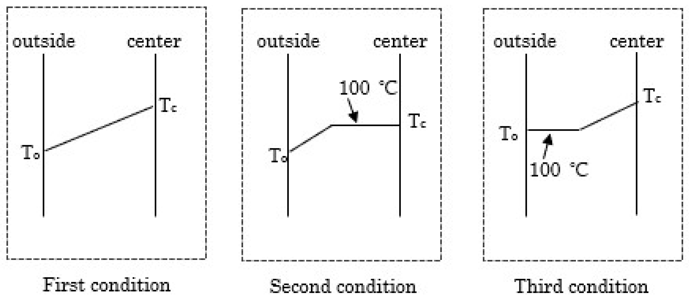
Fourth assumption: The equation from 50 °C to 100 °C was made using the value of the overall temperature of the timber from 50 °C to 110 °C. The results of the overall timber temperature were used from 50 °C because there were few results of ambient temperature up to approximately 50 °C. Three possible cases are shown in Figure 6, where the internal timber temperature was approximately 100 °C because of the stagnation temperature of 100 °C. Equations (9)–(14) show the calculation equation of reduction factor for temperatures from 50 °C to 100 °C.
where
- T1,T2,Tn: temperature;
- y1,y2,yn: Young’s modulus or yield strength.
Figure 6.
Overall timber temperature condition at 100 °C.
Fifth assumption: The equations for the reduction factor of temperature from 50 °C to 100 °C were the average of the slope and intercept that were calculated from the test results for each 1 h and 2 h of heating.
2.1.4. Finite Element Modeling
Figure 11 shows FE models of the compression tests. This analysis was performed using the nonlinear FE analysis software Marc [21]. Table 4 lists the material properties of cedar and larch at the ambient temperature obtained using the determination method described above. The Poisson’s ratios of cedar and larch were taken from the Wood Manufacturing Industry Handbook [22] and reference [23]. Young’s modulus and Poisson’s ratios are related in Equation (15), and the shear modulus was obtained from Equation (16).
where,
- Ex, Ey, Ez: Young’s modulus;
- νxy,νyx, νyz, νzy, νzx, νxz: Poison’s ratios.
- Gxy, Gyz, Gzx: share modulus.
The shape of the element was a cube with a dimension of 5 mm on each side. Surface A was loaded on the YZ plane in the X-direction, and surface B was attached to the YZ plane in the X-direction. All X-Y-Z directions of rotation were fixed. Table 3 lists the material properties at ambient temperature. The material properties at high temperatures were determined using the relationships in Figure 7, Figure 8, Figure 9 and Figure 10. Poisson’s ratio was assumed to not change with temperature. For the value of Young’s modulus and yield strength in the tangential direction, the value of radial direction was used on the basis of a previous study by Shibuya et al. [24].
The anisotropic yield function (from Hill) and stress potential were determined as follows:
where is the equivalent yield stress.
The ratios of actual to isotropic yield (in the preferred orientation) are defined in the array YRDIR for direct yielding and in YRSHR for yield in a shear (the ratio of actual shear yield to isotropic shear yield). Then, –a1–a6 in Equation (17) are defined by Equations (18)–(23).
a1–a6 are Hill’s anisotropy coefficients, expressed in Equations (18)–(23) as the ratio of yield stress in each axial direction.
where the value of shear yield stress in this analysis was the value of reference [22] for both cedar and larch.
Figure 11.
FE models of compression tests.


Table 4.
Material properties used in FE analysis.
| Cedar | Larch | ||
|---|---|---|---|
| Young’s modulus (N/mm2) | EL | 7676.96 | 10,263.70 |
| ER | 413.25 | 298.86 | |
| ET | 413.25 | 298.86 | |
| Poison’s ratios (–) | νLR | 0.40 | 0.48 |
| νRT | 0.90 | 0.93 | |
| νTL | 0.032 | 0.015 | |
| Shear modulus (N/mm2) | GLR | 384.29 | 286.51 |
| GRT | 142.50 | 102.00 | |
| GTL | 380.58 | 286.23 | |
| Yield stress (N/mm2) | σyL | 32.20 | 29.73 |
| σyR | 2.03 | 2.67 | |
| σyT | 2.03 | 2.67 | |
2.2. Embedment Tests
2.2.1. Overview of Embedment Tests
The specimens were made with dowel-type connections of the structural glulam, as shown in Figure 12a–d [13]. The structural glulam (75 × 75 × 300 mm) was processed from three layers of laminae with 25 mm for the specimens compressed parallel to the grain and from five layers of lamina with 30 mm for the specimens compressed perpendicular to the grain, and a steel plate (9 × 75 × 200 mm) and two dowels (φ = 16 length = 75 mm) were inserted. The distance between the steel plate and timber was 15 mm to allow the axial force to be transmitted to the dowels. The material data for the dowels and steel plates are listed in Table 5. In this study, the same types of timber were used for the compression tests. The dowels and steel plates were made of SS400 according to the Japanese Industrial Standards (JIS G 3101) [25]. The test setup and heating method followed those of Kawarabayashi et al. [13].
2.2.2. Finite Element Modeling
During the embedment tests, the stresses in the timber were concentrated around the dowels. Depending on the compression direction, the timber around the dowels exhibited several behaviors. Therefore, three models were used to reproduce this behavior.
Basic Model (for Specimens Loaded Perpendicular and Parallel to the Grain)
The basic model was applied, regardless of the compression direction. Figure 13 illustrates this model. Because the specimen was symmetrical (as shown in Figure 12), it was modeled from the load surface up to 100 mm of the steel plate (i.e., half of the steel plate). Dowels of the length, excluding the tapered part, were modeled. The diameter of the dowels was the same as that of the inserted timber hole in the design. However, the reality was that the dowel was slightly smaller than the diameter of the inserted timber hole. When the dowel and timber hole have the same diameter in the analysis, friction cannot be considered because they have a common node; therefore, the dowel diameter was set to φ = 15.98 mm. For the dowel area and the timber part with a dowel circumference of 5 mm, the element shape size was 1 mm per side. The element shape size was 5 mm per side for the steel plate and the other timber parts. The surface “Ae” was loaded in the X direction on the YZ plane, the surface “Be” was fixed in the X direction on the YZ plane, and each rotation direction of all X-Y-Z axes was fixed. The contact conditions were that the steel plate and dowel were bonded together, and the timber and dowel were in contact with each other, with a coefficient of friction of 0.001. Because timber failure occurred before the yield of the steel connectors in all embedment test specimens, the steel connectors were assumed to be in the elastic range in these analyzes. The Young’s modulus was set at 205 kN/mm2, and the Poisson’s ratio of the steel plate and dowels was set at 0.3. The effect of temperature on steel plate and dowels was neglected because the Young’s modulus of the steel changed negligibly up to 100 °C. The relationships between the material properties and the temperatures of the timber were the same as those obtained with the FE analysis of the compression tests.
Split Model (for Specimens Loaded Perpendicular to the Grain)
For the specimens loaded perpendicular to the grain, splitting of the timber occurred around the hole along the tree ring. The split model was used for the cases where the splitting of the timber around the hole occurred, as shown in Figure 14. This model was the same as the basic model, except that the timber was divided into two pieces at this point. The coefficient of friction of the contact surface between the pieces of timber was 0.3.
Damage Zone Model (for Specimens Loaded Parallel to the Grain)
The damage zone model was used to account for the effects of the damage zones. A damage zone is an area of low stiffness near the butt ends under compression parallel to the grain [26,27,28,29], and it is assumed to be caused by the roughness of the surface when the timber is cut [30]. Therefore, the length of the damage zone depends on the processing method used. Totsuka et al. proposed a method for evaluating the initial stiffness of the damage zone in embedment tests [5]. The length of the damage zone was calculated using Equation (24). The Young’s modulus of the damage zone was 1.8% of the Young’s modulus of timber parallel to the grain [5].
where,
- x: length of the damage zone;
- A’: horizontal projected area of the contacted area;
- k: coefficient according to the processing method;
- xs: length of the damage zone of the reference specimen.
Figure 15 shows the damage zone model. There is no defined method for setting up the damage zone in the FE analysis. Therefore, the area of the damage zone was designated as the contact area, which corresponds to the cross-sectional area of the timber surface at the center of the dowel, ±45° in the compression direction, as shown in Figure 15a,b. The length of the damage zone was calculated using a separate area, as shown in Figure 15b. The value of A’ in this model corresponds to the equivalent cross-section (mm2) 1 or 2 in Figure 15b [5]. The shape of the damage zone area was determined because the effects occurred only at the compressive force between the dowel and the timber.
Table 6 lists the material properties of the damage zones. Since the material properties of the damage zone must only reduce the Young’s modulus parallel to the grain, the Poisson’s ratio of the damage zone should be determined by considering the relationship in Equation (15). The Poisson’s ratios, which can be calculated from the Poisson’s ratios in Table 3 and Young’s modulus, were determined not to exceed 1.
3. Results
3.1. Compression Results
Figure 16 and Figure 17 show the results of the numerical analysis of the compression tests at ambient temperature. The values of the explanatory notes in parentheses in Figure 17 indicate the set plastic modulus (N/mm2). In the test results of the compression parallel to the grain, the load gradually decreased after yielding. Because the range between yield point and the maximum load is very small for compression parallel to the grain, the numerical results parallel to the grain discuss the behavior of elastic and yield points. Therefore, the plastic modulus for evaluating the yield point in the numerical results was set to an extremely small value. The numerical results in the parallel direction represent the initial stiffness and yield point of the test results, as shown in Figure 16. Figure 17a,b compares the test results (legend “Exp.”) and several analytical results with varying plastic moduli perpendicular to the grains. The values of plastic stiffness of the numerical results (legend “plastic (Exp.)-anal”), obtained by using the plastic modulus obtained by the bi-linearization of the test result, were larger than those of the test results. Figure 18, Figure 19, Figure 20 and Figure 21 show the numerical results of compression tests at high temperatures. The optimal plastic modulus at high temperatures was determined by the same method used for the optimal plastic modulus at ambient temperature. The FE results were well reproduced in the test behavior. The results show that the Young’s modulus and yield stress at high temperatures determined in Section 2.2 can reproduce the test values.
3.2. Embedment Results
Figure 22, Figure 23, Figure 24, Figure 25, Figure 26 and Figure 27 show the numerical results of the load–displacement relationship. For the numerical results of the basic model in the parallel direction, the initial stiffness of the numerical results was higher than that of the test results (Figure 22). However, the damage zone model reproduced the test results. However, the 100 °C numerical result using the damage zone model was higher than the test results (Figure 24).
4. Discussion
4.1. Compression Behavior
We focused our compression test on one element in the timber, perpendicular to the grain, in order to clarify why the post-yield behavior of the numerical results was higher when a test post-yield slope was specified for the plastic modulus. Figure 28a,b shows the stress of one element at the center of the specimen, where X is the compression direction, Y is the width direction, and Z is the depth direction. The compressive stress component is indicated by a positive value (X, Y, and Z are in the same direction as Figure 11). The compression components σyy and σzz increased after the yield point. When σyy and σzz did not occur, the equivalent stress had the same value. Therefore, compared to σyy and σzz not occurring (Figure 28b, red line), the equivalent stress due to σyy and σzz decreased, even after the yield point (Figure 28b, black line). Because the plastic modulus determined in the test results included the effect of decreasing after the yield point, the behavior after the yield point increased when the test value was set in the plastic modulus of the FE analysis. In the 2D numerical results by Oudjene et al. [9], the plastic stiffness was not greater than those of the test results as the plastic modulus was corrected to replicate the equivalent stress–equivalent strain relationship in compression tests. Therefore, the optimal plastic modulus for the FE analysis should be determined by comparing the test results. The optimal plastic modulus was E1/140 N/mm2 for the cedar specimens (Plastic (5)-anal. in Figure 17a) or E1/100 N/mm2 for the larch specimens (Plastic (2)-anal. in Figure 17b).
4.2. Embedment Behavior
Figure 29 shows the deformation diagram, and Figure 30 and Figure 31 show the stress distributions on the X-axis at ambient temperature. Figure 30 and Figure 31 show the stress diagrams at the maximum load parallel to the grain and at the yield load perpendicular to the grain. Figure 32 shows the X-axis stress distributions of the split model at 100 °C.
4.2.1. Embedment Behavior of Parallel to the Grain
The numerical result of 100 °C using the damage zone model was higher than the test results (Figure 24). This was because the temperature of the bearing around the dowel was higher than that of the rest of the bearing part. The temperature of the bearing part was higher than that of the rest of the timber because it was heated by the dowel. The higher the temperature, the lower the influence of the damage zone, when the heating by the dowel is taken into account. The deformation of the load-bearing part around the dowel was more dominant in the damage zone model than in the basic model (Figure 29). When the deformation in the FE analysis becomes large (especially in the contact area), it is impossible to obtain a convergent solution, and the analysis may terminate. Although the material properties in this analysis were given in bilinear form, the post-yield stiffness can be seen in the analysis results (Figure 22, Figure 23 and Figure 24) until the analysis terminates. In the basic model, the compressive stress around the dowel was concentrated in a small area (Figure 30). Conversely, in the damage zone model, the compressive stress occurred in the entire area of the damaged zone. Because compressive stress was transmitted from the steel plate to the middle of the dowel on the timber foundation, it was assumed that the bending deflection of the dowel could be larger for the basic model than in the damage zone model.
4.2.2. Embedment Behavior Perpendicular to the Grain
In the basic model, tensile stress occurred in the X-axis around the top and bottom of the dowel hole, as shown in Figure 31b. Because cleavage occurred in this area during the tests, the stress distribution after cleavage was considered in the split model. Although there were differences in the stress distribution of both models between Figure 31a,b, there was little difference in the stiffness or yield load, as shown in Figure 25. This indicates that cleaving had a minimal effect on the stiffness and yield load in the test and that the FE analysis using the basic model can approximate the embedment behavior in terms of the stiffness and yield load of the timber around the dowel. The distribution of shear stress along the XY-axis of a specimen loaded perpendicular to the grain at ambient temperature is shown in Figure 33a. The shear stress distribution in Figure 33a represents the basic model at maximum load. Figure 33b shows the corresponding image of the specimen post-test. A comparison of the area of maximum shear stress in Figure 33a and the location of cleavage in Figure 33b revealed similarities. These findings suggest that the analytical results in the basic model accurately reproduced the initiation location of cleavage. At ambient temperature, the area of high compressive stress was triangularly distributed toward the center (Figure 31), whereas at high temperatures, the distribution was square away from the center (Figure 32). This indicates that the dowel bended at ambient temperatures, whereas at high temperatures, the entire dowel transferred stress to the bearing part. This indicates a difference in the fracture properties of the bearing with increasing temperature.
5. Conclusions
In this study, 3D elastoplastic FE analyses of compression tests and embedment tests in timber were performed at ambient and high temperatures. The results provide a deep understanding of the analysis method and the behavior of the compression and embedment tests, as summarized below.
5.1. FE Analysis of Compression Tests
The proposed analytical method successfully reproduced the initial stiffness and yield points of the test results. When the plastic modulus, obtained from the stress–strain relationship of the test results, was set to the plastic modulus, the stiffness after the yield point was higher in the numerical results than that in the test results. This was because the stress on the Y-axis and Z-axis increased after the yield point, thereby increasing the equivalent yield stress.
5.2. FE Analysis of Embedment Tests
Three types of FE models were proposed. The first model was the basic one, the second was the split model that incorporated cleavage in the division of the wood into two pieces, and the third was the damage zone model that accounted for the reduced stiffness in the vicinity of a dowel.
The damage zone model was able to reproduce the test behavior parallel to the grain. When the damage zone was not considered, the initial stiffness of the numerical results in compression parallel to the grain was significantly higher than that of the test results. However, the temperature of the bearing part was lower than that of the rest of the timber because it was heated by the dowel. The higher the temperature, the lower the influence of the damage zone, when the heating by the dowel was taken into account. The numerical results of the basic and split models in the perpendicular direction reproduced the test stiffness and behavior after the yield point. In the basic model, the tensile stresses occurred in the X-axis around the top and bottom of the dowel hole. Because cleavage occurred in this area during testing, the stress distribution after cleavage was considered in the split model.
At ambient temperatures, the area of high compressive stress was triangularly distributed toward the center, whereas at high temperatures, the distribution was square away from the center. This indicates that the dowel bent at ambient temperatures, whereas at high temperatures, the entire dowel transferred stress to the bearing part. This indicates a difference in the fracture properties of the bearing with increasing temperature.
The methodology advanced in this study failed to replicate the maximum compressive capacity and timber splitting, as the purview of this study pertained to elastic distortions and the yield points. Further refinement of the framework is imperative when investigating fracture mechanics.
In the future, application of the results of this study may help predict the stress distribution of timber beam–column connections with dowels at ambient and high temperatures.
Author Contributions
Y.K., M.T. and T.H. designed the study. Y.K. performed the analyses. Y.K. analyzed the data. Y.K. and M.T. were the major contributors to writing the manuscript. All authors contributed to the interpretation and discussion of the results. All authors have read and agreed to the published version of the manuscript.
Funding
This work was supported by JSPS KAKENHI (grant numbers JP19H02281 and JP22H01636).
Institutional Review Board Statement
Not applicable.
Informed Consent Statement
Not applicable.
Data Availability Statement
Not applicable.
Acknowledgments
The computation was carried out using computer resources offered under the category of General Projects by the Research Institute for Information Technology, Kyushu University.
Conflicts of Interest
The funders had no role in the study design; collection, analyses, or interpretation of data; writing of the manuscript; or decision to publish the results.
References
- Zhang, C.; Guo, H.; Jung, K.; Harris, R.; Chang, W. Using self-tapping screw to reinforce dowel-type connection in a timber portal frame. Eng. Struct. 2019, 178, 656–664. [Google Scholar] [CrossRef]
- Schneid, E.; de Moraes, P.D. Grain angle and temperature effect on embedding strength. Constr. Build Mater. 2017, 150, 442–449. [Google Scholar] [CrossRef]
- Yurrita, M.; Cabrero, J.M. New criteria for the determination of the parallel-to-grain embedment strength of wood. Constr. Build Mater. 2018, 173, 238–250. [Google Scholar] [CrossRef]
- Van Blokland, J.; Florisson, S.; Schweigler, M.; Ekevid, T.; Bader, T.K.; Adamopoulos, S. Embedment properties of thermally modified spruce timber with dowel-type fasteners. Constr. Build Mater. 2021, 313, 125517. [Google Scholar] [CrossRef]
- Totsuka, M.; Hayakawa, J.; Aoki, K.; Inayama, M. Evaluation of stiffness parallel to grain of wood based on strongest link model. J. Struct. Constr. Eng. 2022, 87, 770–779. [Google Scholar] [CrossRef]
- Johansen, K.W. Theory of timber connections. Int. Assoc. Bridge Struct. Eng. 1949, 9, 249–262. [Google Scholar]
- EN 1995-7-2 Eurocode5: Design of Timber Structures; European Union: Bruxelles, Belgium, 1995; p. 51.
- Kawarabayashi, F.; Kikuchi, T.; Yotumoto, N.; Totsuka, M.; Hirashima, T.; Nakayama, Y. Load-Bearing Fire Tests of Structural Glulam Timber Frame of Larch with Dowel Connections Part 1: Outlines of the tests and Results of Ambient tests. In Proceeding of Architectural Research Meetings; Kanto Chapter; Architectural Institute of Japan: Tokyo, Japan, 2022; p. 3. [Google Scholar]
- Oudjene, M.; Khelifa, M. Elasto-plastic constitutive law for wood behavior under compressive loadings. Constr. Build Mater. 2009, 23, 3359–3366. [Google Scholar] [CrossRef]
- Xu, B.H.; Bouchair, A.; Taazount, M.; Vega, E.J. Numerical and experimental analyses if multiple-dowel steel-to-timber joints in tension perpendicular to grain. Eng. Struct. 2009, 31, 2357–2367. [Google Scholar] [CrossRef]
- Audebert, M.; Dhima, D.; Bouchaïr, A.; Frangi, A. Review of experimental data for timber connections with dowel-type fasteners under standard fire exposure. Fire Safe. J. 2019, 107, 217–234. [Google Scholar] [CrossRef]
- Peng, L.; Hadjisophocleous, G.; Mehaffey, J.; Mohammad, M. Fire resistance performance of unprotected wood–wood–wood and wood–steel–wood connections: A literature review and new data correlations. Fire Saf. J. 2010, 45, 392–399. [Google Scholar] [CrossRef]
- Kawarabayashi, F.; Kikuchi, T.; Totsuka, M.; Hirashima, T. Embedding behaviors of a doweled connection in structural glulam timbers at high temperature. J. Struct. Constr. Eng. 2022, 87, 498–509. [Google Scholar] [CrossRef]
- Kikuchi, T.; Yotsumoto, J.; Kawarabayashi, F.; Ishida, Y.; Totsuka, M.; Hirashima, T. Experimental study on fire performance of glulam timber frames (part 1)—Temperature and charring behavior of the beam-column connections exposed to standard fire heating for more than 1 hour. J. Struct. Constr. Eng. 2022. In press. [Google Scholar] [CrossRef]
- Cachim, P.B.; Franssen, J.M. Numerical modelling of timber connections under fire loading using a component model. Fire Saf. J. 2009, 44, 840–853. [Google Scholar] [CrossRef]
- Nakayama, Y.; Kikuchi, T.; Totsuka, M.; Hirashima, T. Numerical model for non-linear M-θ relationships of dowel-type timber connections exposed to fire. In Proceedings of the 12th International Conference on Structures in Fire, Hong Kong, China, 30 November–2 December 2022; pp. 1064–1075. [Google Scholar]
- Audebert, M.; Dhima, D.; Taazount, M.; Bouchaïr, A. Experimental and numerical analysis of timber connections in tension perpendicular to grain in fire. Fire Saf. J. 2014, 63, 125–137. [Google Scholar] [CrossRef]
- Khelifa, M.; Khennane, A.; Ganaoui, M.E.I.; Rogaume, Y. Analysis of the behavior of multiple dowel timber connections in fire. Fire Saf. J. 2014, 68, 119–128. [Google Scholar] [CrossRef]
- Sawata, K.; Yasumura, M. Determination of embedding strength of wood for dowel-type fasteners. J. Wood Sci. 2002, 48, 138–146. [Google Scholar] [CrossRef]
- Inayama, M. Mokuzainomerikomirirontosonoouyou-jinseinikitaishitamokushituramensetugoubunotaishinnsekkeihounikannsurukenkyuu. Ph.D. Thesis, The University of Tokyo, Tokyo, Japan, 1991. [Google Scholar]
- MSC.MARC User’s Manual. Vol. A: Theory and User Information; MSC Software Corporation: Stockholm, Sweden, 2017.
- Wood Industry Handbook–Part 2 Wood Properties 174, 3rd ed.; Maruzen Co.: Ichikawa, Japan, 1982.
- Hirosue, M.; Nakagome, T.; Fujioka, T.; Kanbe, W.; Kamakura, M. An analytical study for mode 1 fracture toughness of woods with FEM considered orthotropic anisotropy Part 3 analysis result. In Summary of Technical Papers of the Annual Meeting; Architectural Institute of Japan: Tokyo, Japan, 2011; pp. 217–218. [Google Scholar]
- Shibuya, T.; Takino, A.; Miyamoto, Y. Study on wood material model including orthotropy in 3D finite element analysis. In Summary of Academic Papers DVD; Architectural Institute of Japan: Tokyo, Japan, 2012; pp. 679–680. [Google Scholar]
- Japanese Industrial Standard G 3101; Rolled Steels for General Structure. Japanese Standards Association: Tokyo, Japan, 2020.
- Zink, A.G.; Davidson, R.W.; Hanna, R.B. Strain measurement in wood using a digital image correlation technique. Wood Fiber Sci. 1995, 27, 346–359. [Google Scholar]
- Xavier, J.; de Jesus, A.M.P.; Morais, J.J.L.; Pinto, J.M.T. Stereovision measurements on evaluating the modulus of elasticity of wood by compression tests parallel to the grain. Constr. Build Mater. 2011, 26, 207–215. [Google Scholar] [CrossRef]
- Martin, B.; Jan, T.; Václav, S.; Jaromír, M.; Peter, R. Standard and non-standard deformation behavior of European beech and Norway spruce during compression. Holzforschung 2015, 69, 1107–1116. [Google Scholar] [CrossRef]
- Totsuka, M.; Jockwer, R.; Aoki, K.; Inayama, M. Experimental study on partial compression parallel to grain of solid timber. J. Wood. Sci. 2021, 67, 39. [Google Scholar] [CrossRef]
- Totsuka, M.; Jockwer, R.; Kawahara, H.; Aoki, K.; Inayama, M. Experimental study of compressive properties parallel to grain of glulam. J. Wood Sci. 2022, 68, 33. [Google Scholar] [CrossRef]
Figure 1.
Test information of compression tests. (a) Set up of compression test; (b) lamina configuration.
Figure 1.
Test information of compression tests. (a) Set up of compression test; (b) lamina configuration.

Figure 2.
Temperature measurement position.
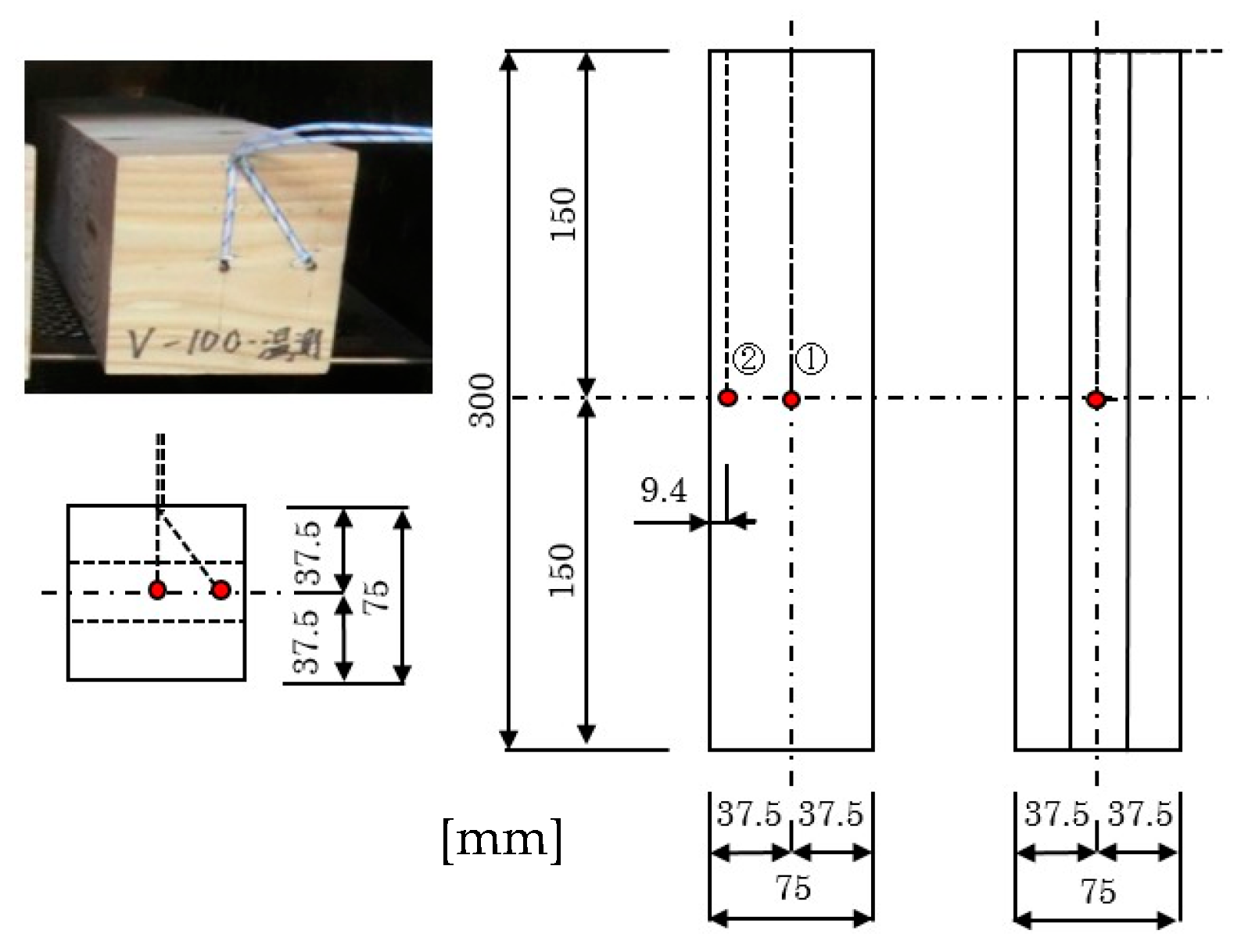
Figure 4.
Flowchart of determining yield point.
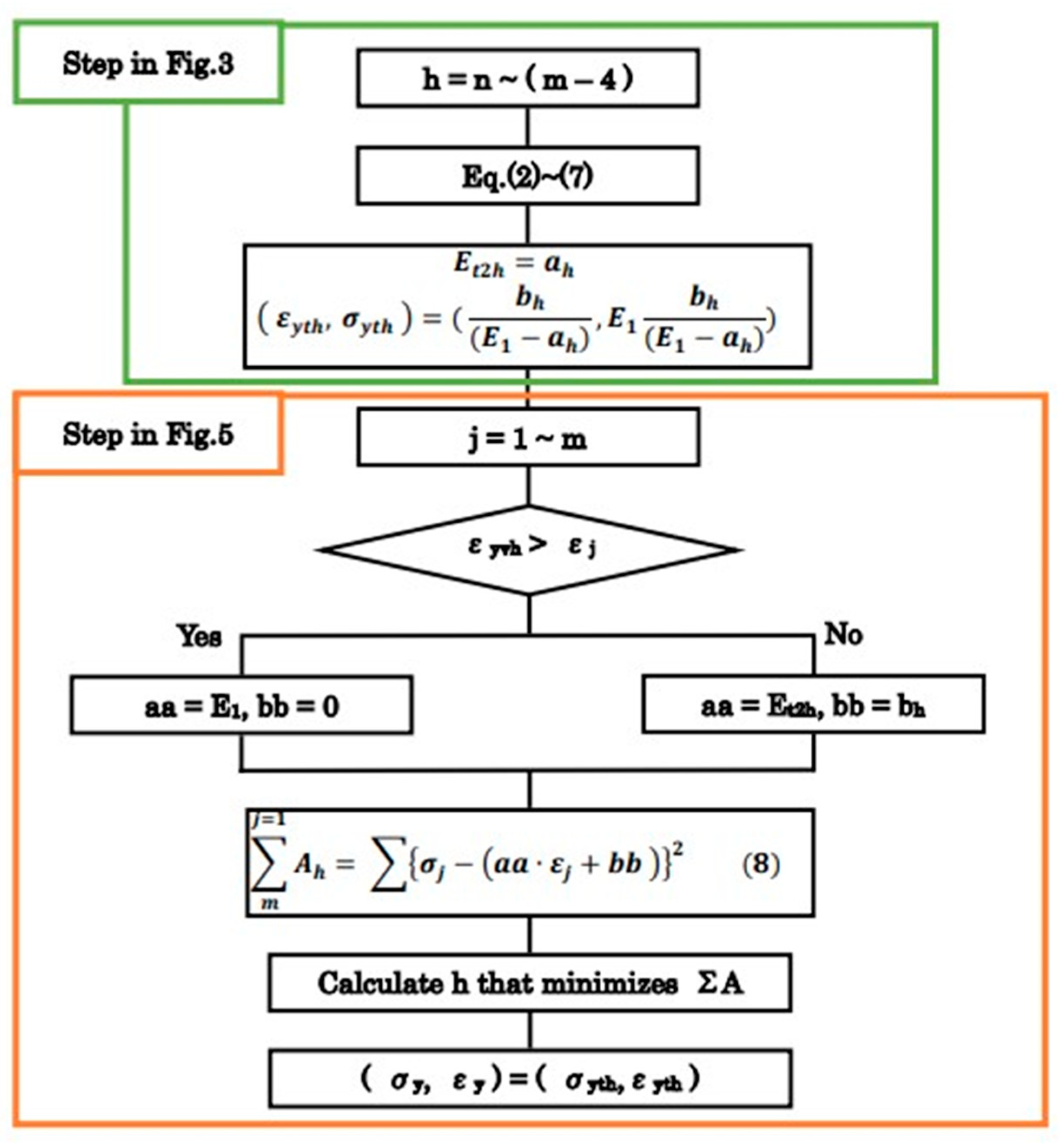
Figure 5.
Illustration of Equation (8).
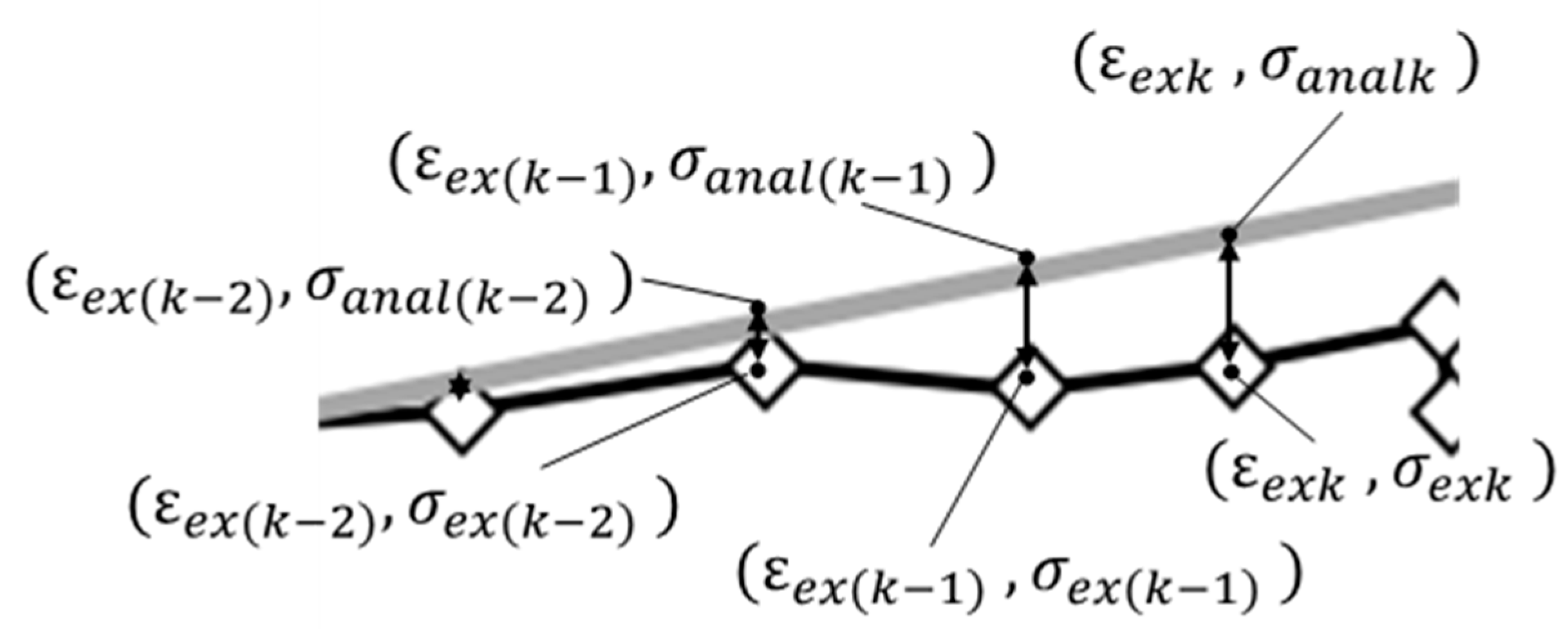
Figure 7.
Influence of temperature on Young’s modulus parallel.
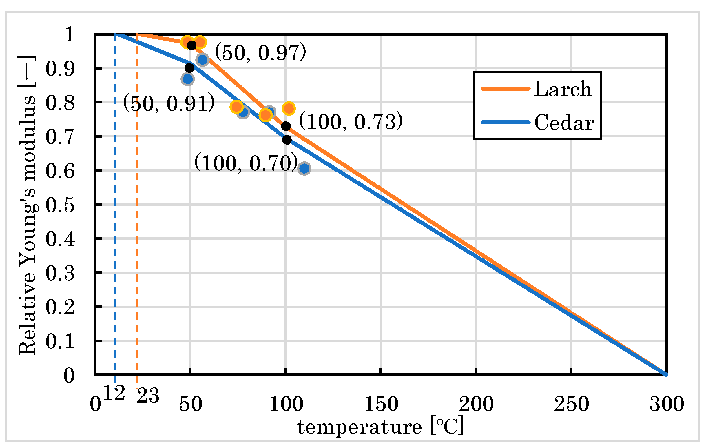
Figure 8.
Reduction factor for the yield strength parallel.
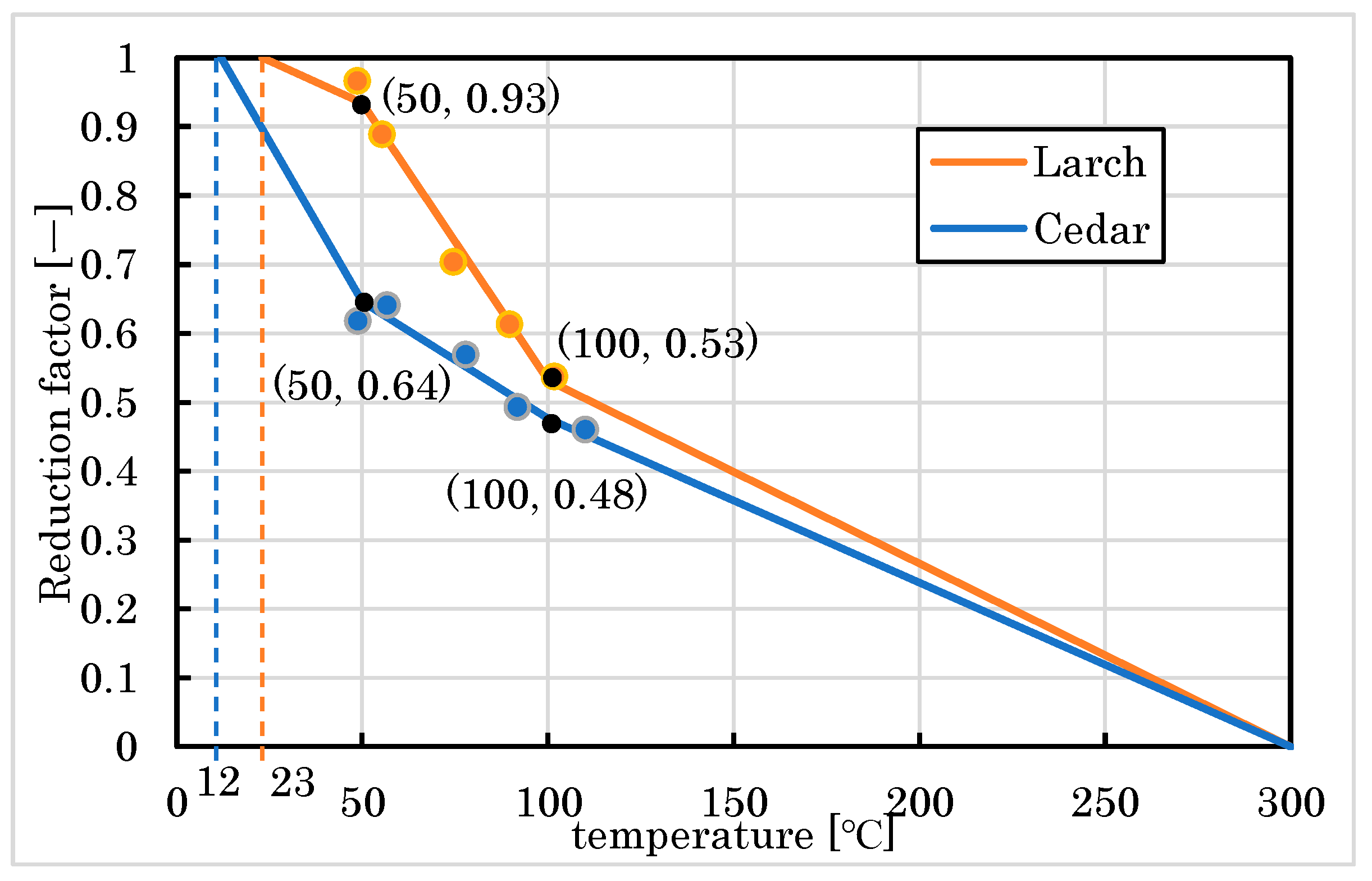
Figure 9.
Influence of temperature on Young’s modulus perpendicular.
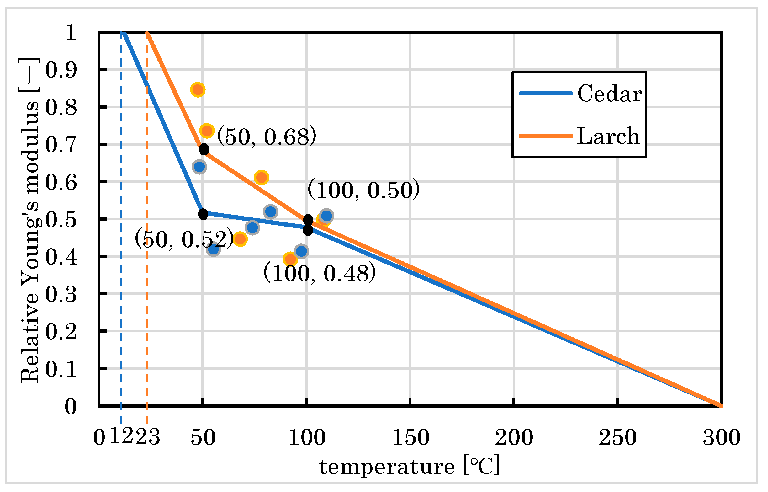
Figure 10.
Reduction factor for the yield strength perpendicular.
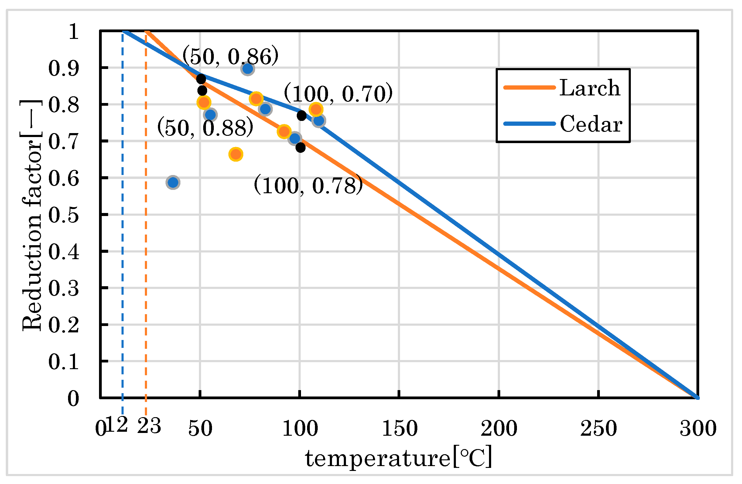
Figure 12.
Specimens of the embedment test.
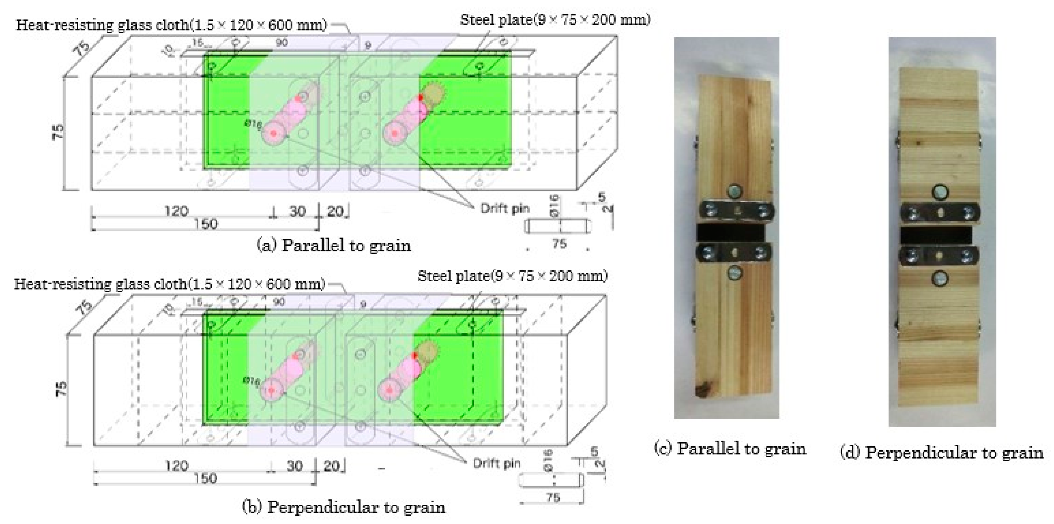
Figure 13.
The basic model of the embedment tests.

Figure 14.
Split model of the embedment tests.
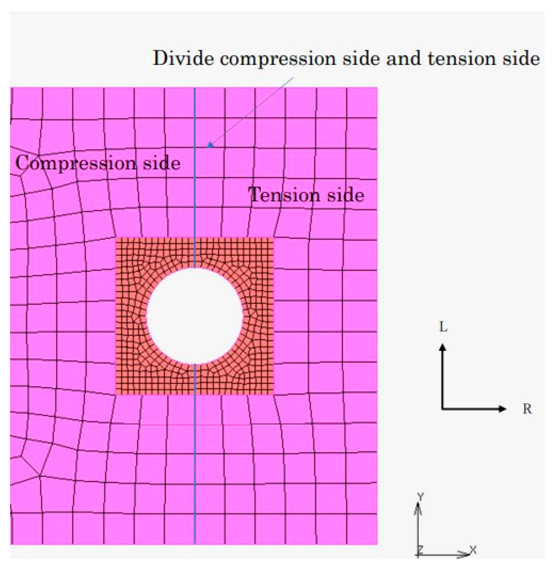
Figure 15.
Damage zone model of embedment tests.
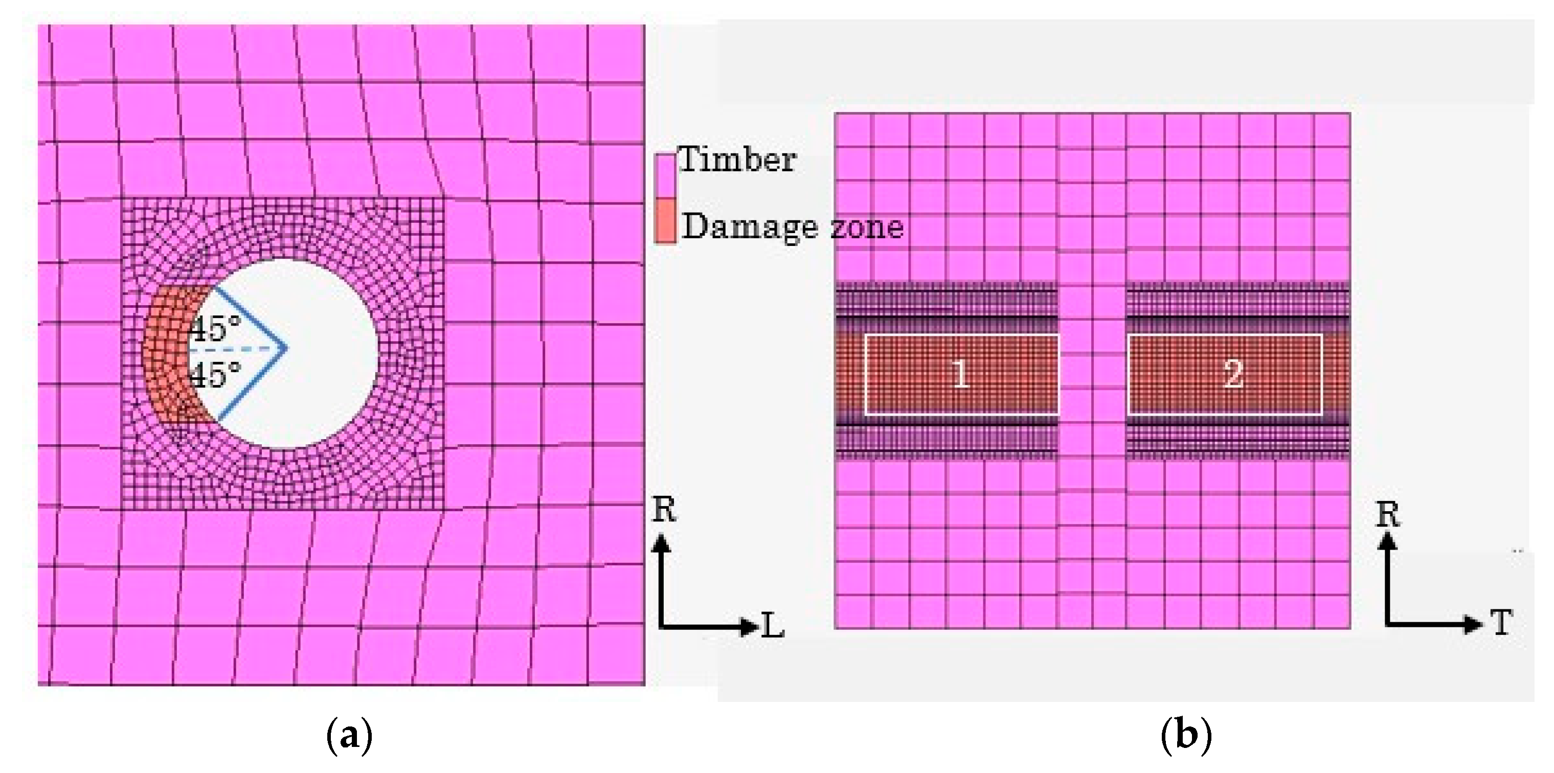
Figure 16.
Load–displacement relationships parallel to the grain at ambient temperature. (a) Cedar; (b) larch.
Figure 16.
Load–displacement relationships parallel to the grain at ambient temperature. (a) Cedar; (b) larch.

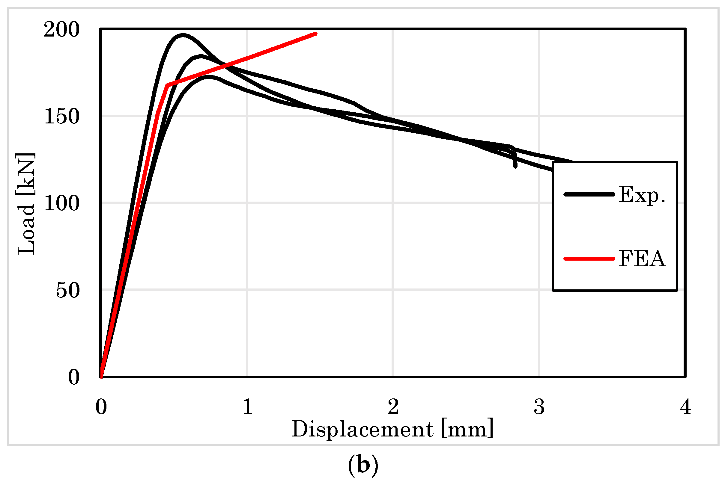
Figure 17.
Load–displacement relationship perpendicular to the grain at ambient temperature. (a) Cedar; (b) larch.
Figure 17.
Load–displacement relationship perpendicular to the grain at ambient temperature. (a) Cedar; (b) larch.

Figure 18.
Load–displacement relationship parallel at 60 °C heating temperature. (a) Cedar; (b) larch.
Figure 18.
Load–displacement relationship parallel at 60 °C heating temperature. (a) Cedar; (b) larch.
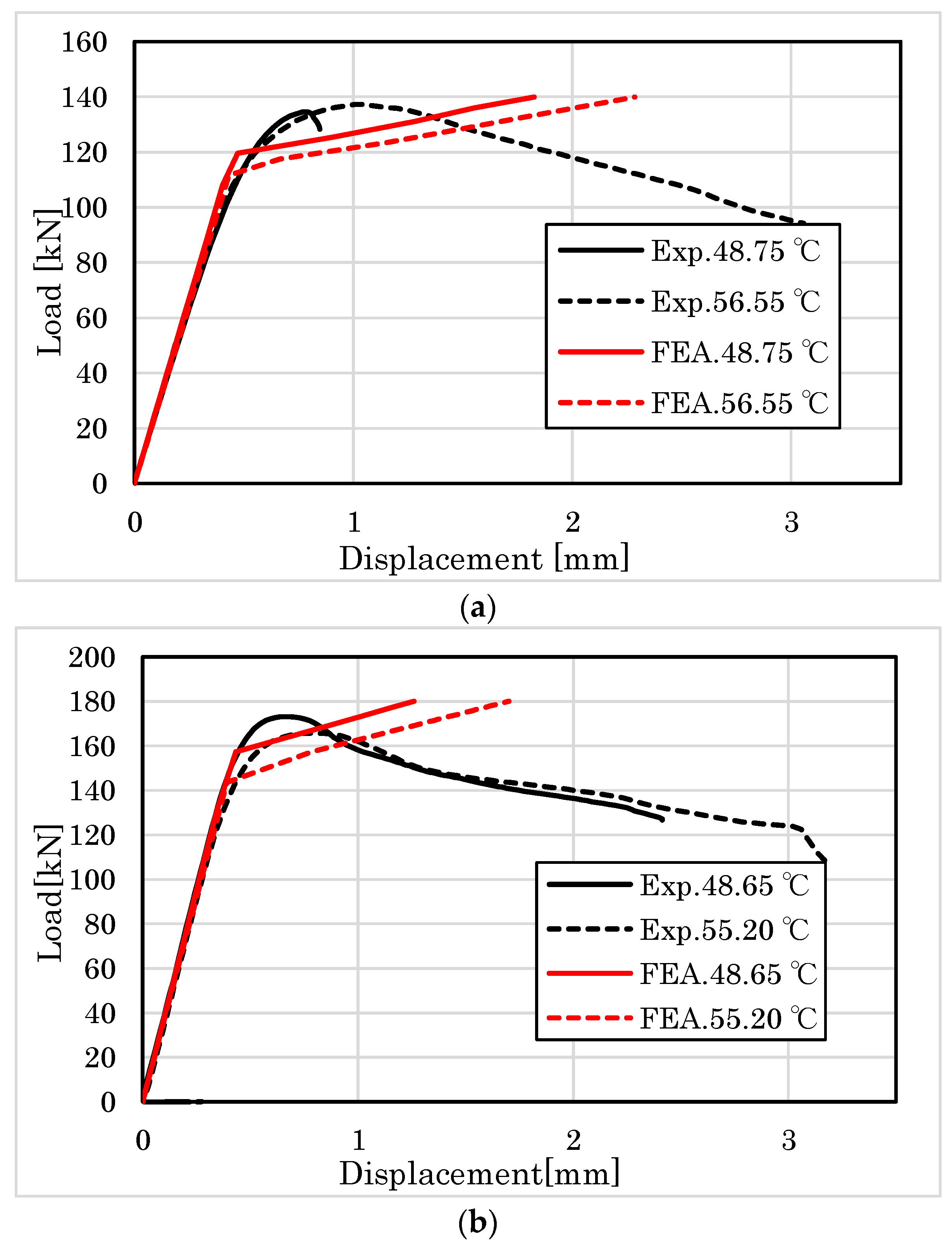
Figure 19.
Load–displacement relationship parallel at 100 °C heating temperature. (a) Cedar; (b) larch.
Figure 19.
Load–displacement relationship parallel at 100 °C heating temperature. (a) Cedar; (b) larch.
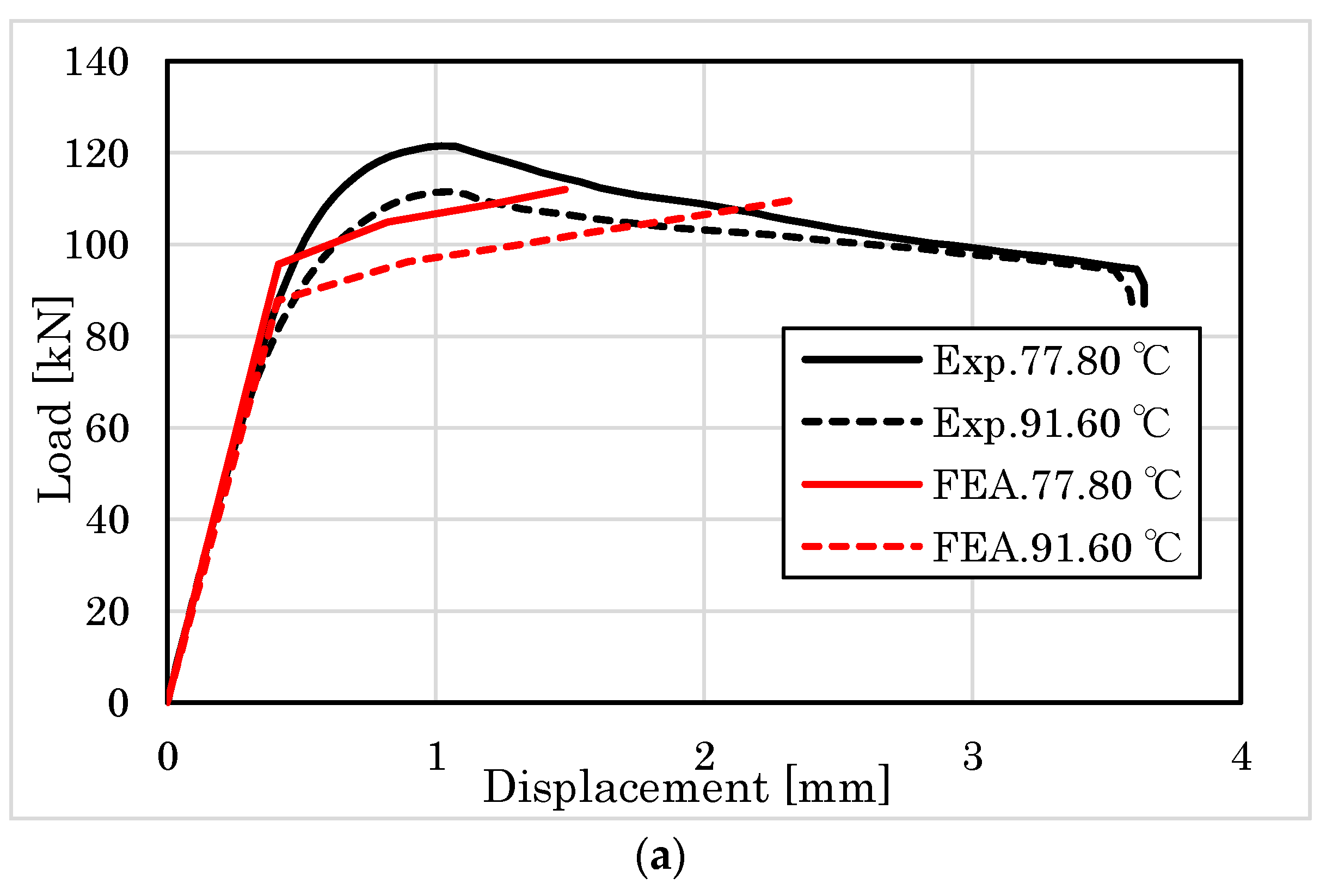

Figure 20.
Load–displacement relationship perpendicular at 60 °C heating temperature. (a) Cedar; (b) larch.
Figure 20.
Load–displacement relationship perpendicular at 60 °C heating temperature. (a) Cedar; (b) larch.
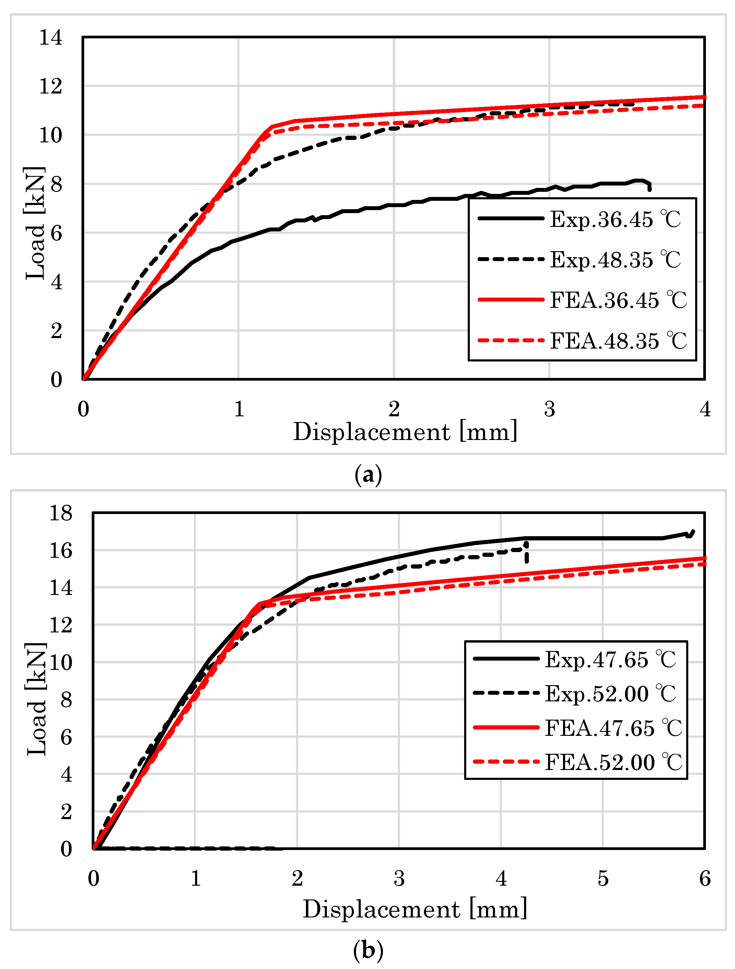
Figure 21.
Load–displacement relationship perpendicular at 100 °C heating temperature. (a) Cedar; (b) larch.
Figure 21.
Load–displacement relationship perpendicular at 100 °C heating temperature. (a) Cedar; (b) larch.
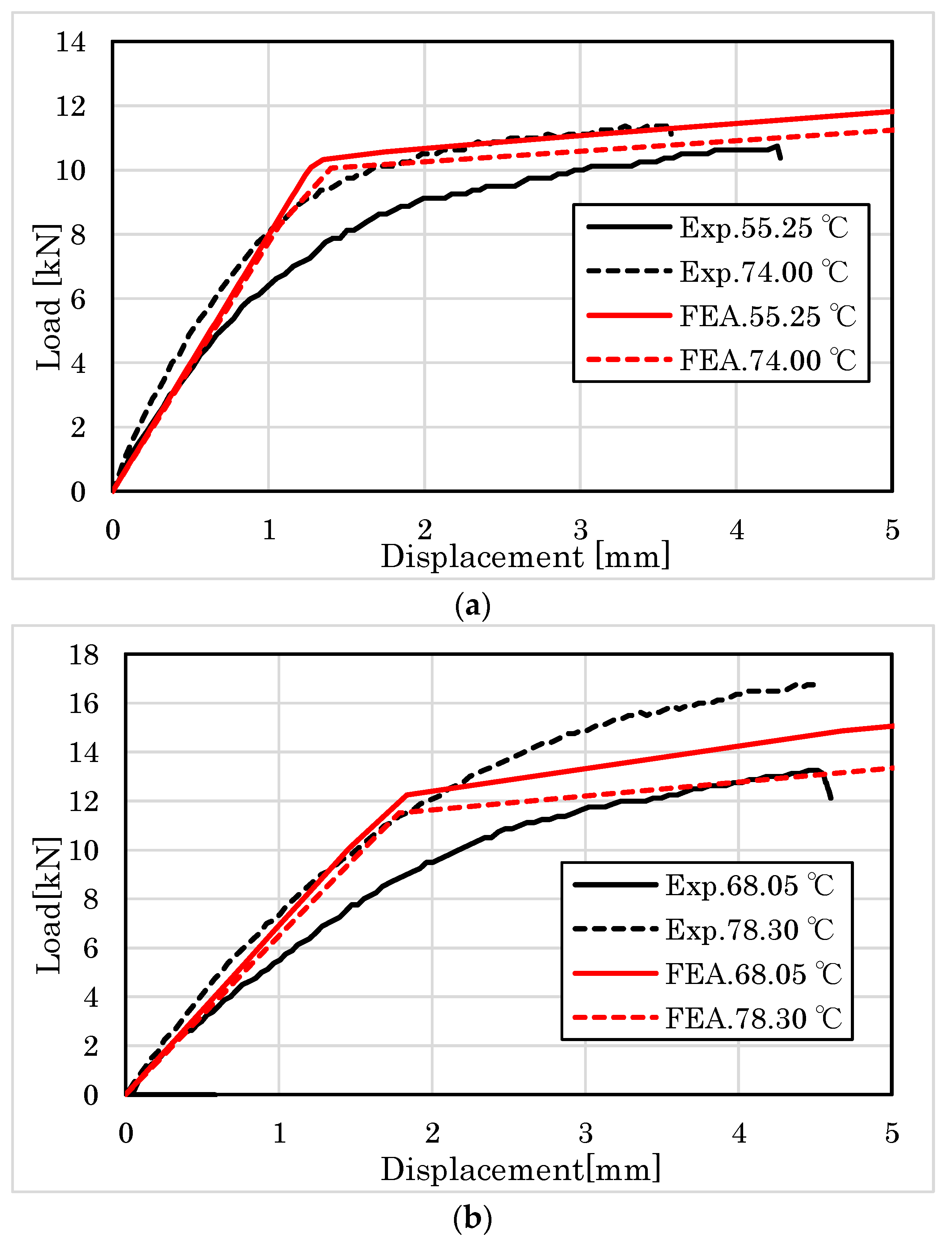
Figure 22.
Load–displacement relationship parallel at ambient temperature. (a) Cedar; (b) larch.
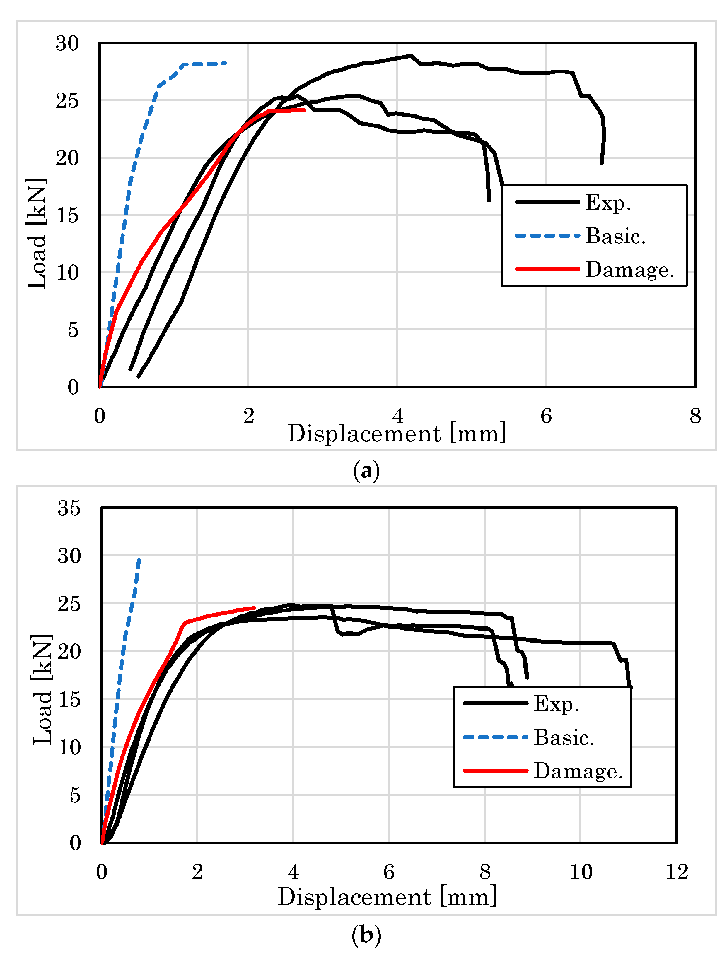
Figure 23.
Load–displacement relationship parallel at 60 °C heating temperature. (a) Cedar; (b) larch.
Figure 23.
Load–displacement relationship parallel at 60 °C heating temperature. (a) Cedar; (b) larch.
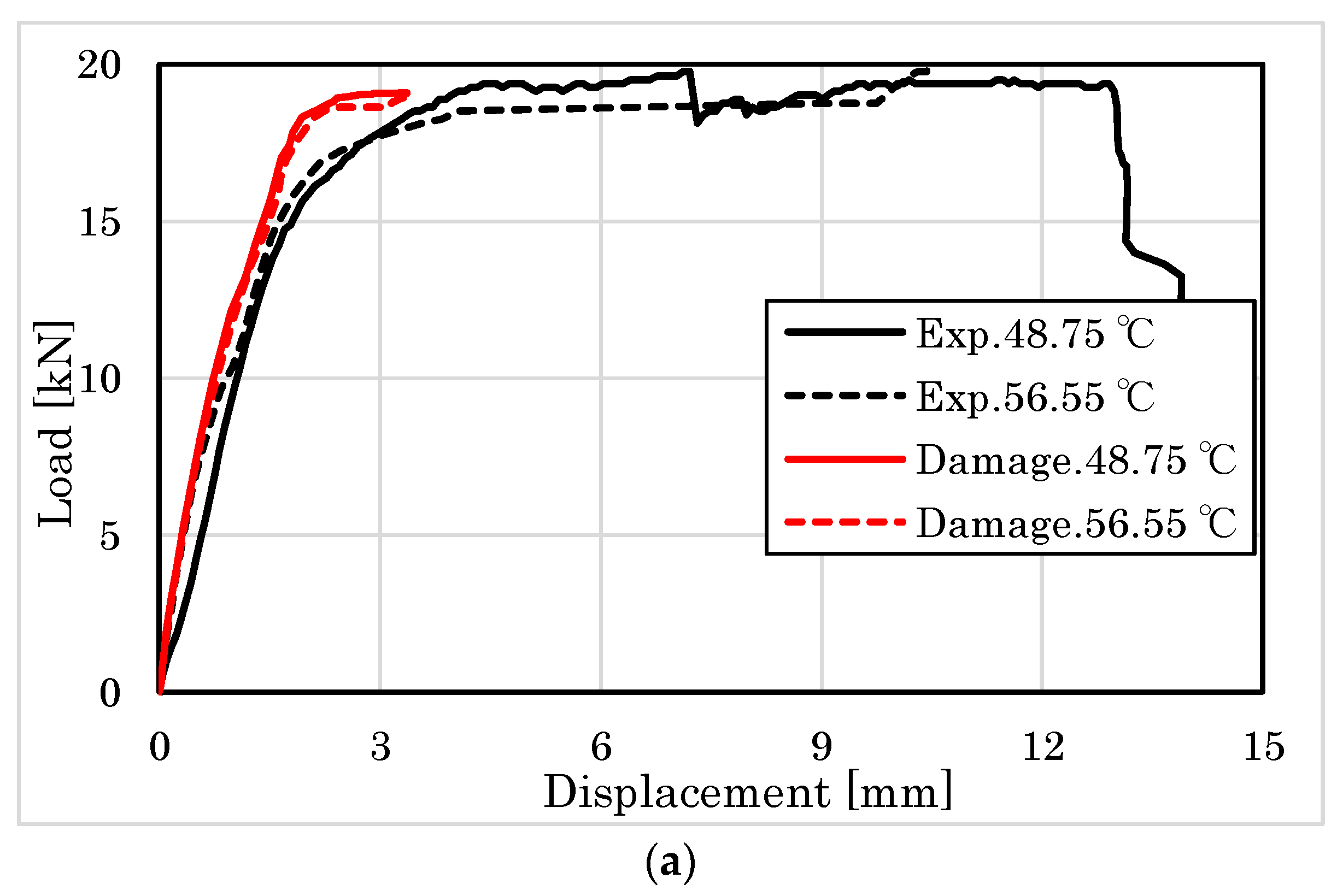
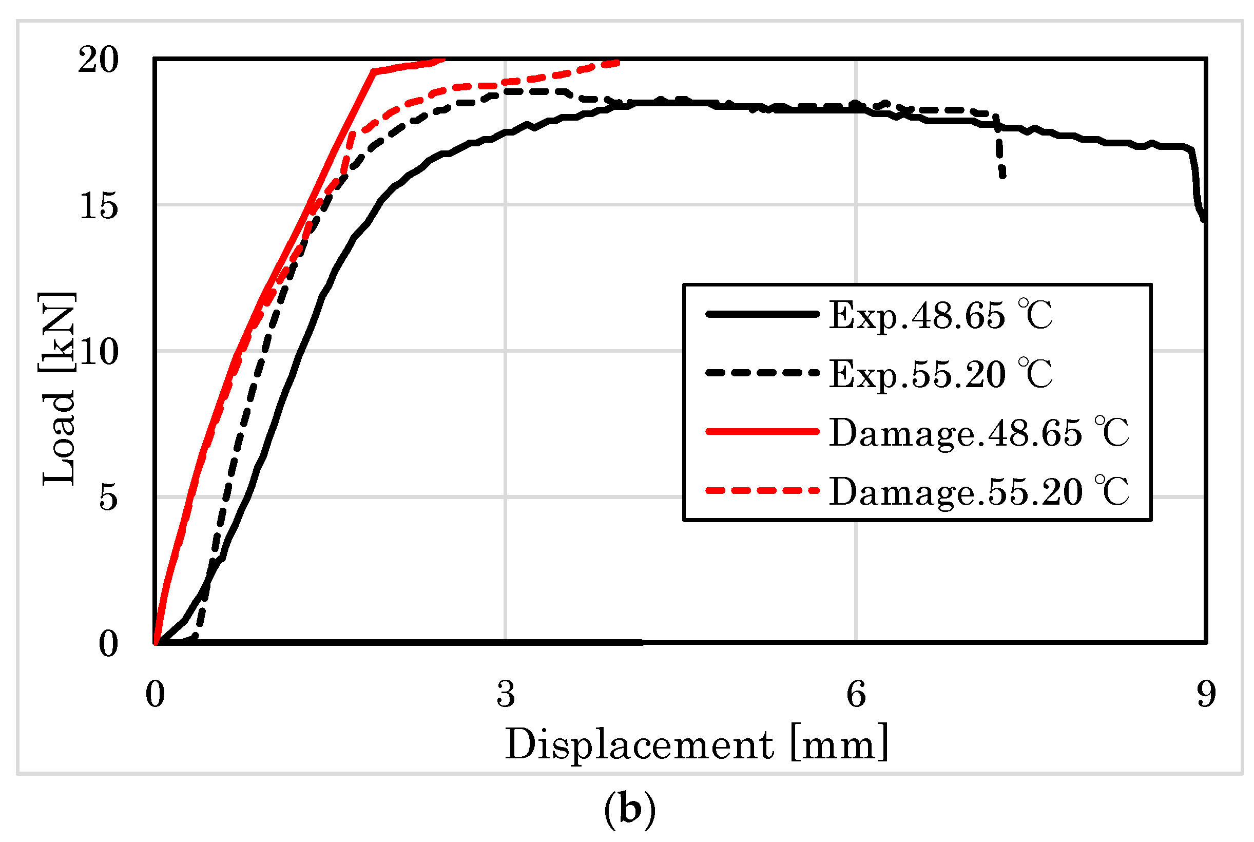
Figure 24.
Load–displacement relationship parallel at 100 °C heating temperature. (a) Cedar; (b) larch.
Figure 24.
Load–displacement relationship parallel at 100 °C heating temperature. (a) Cedar; (b) larch.
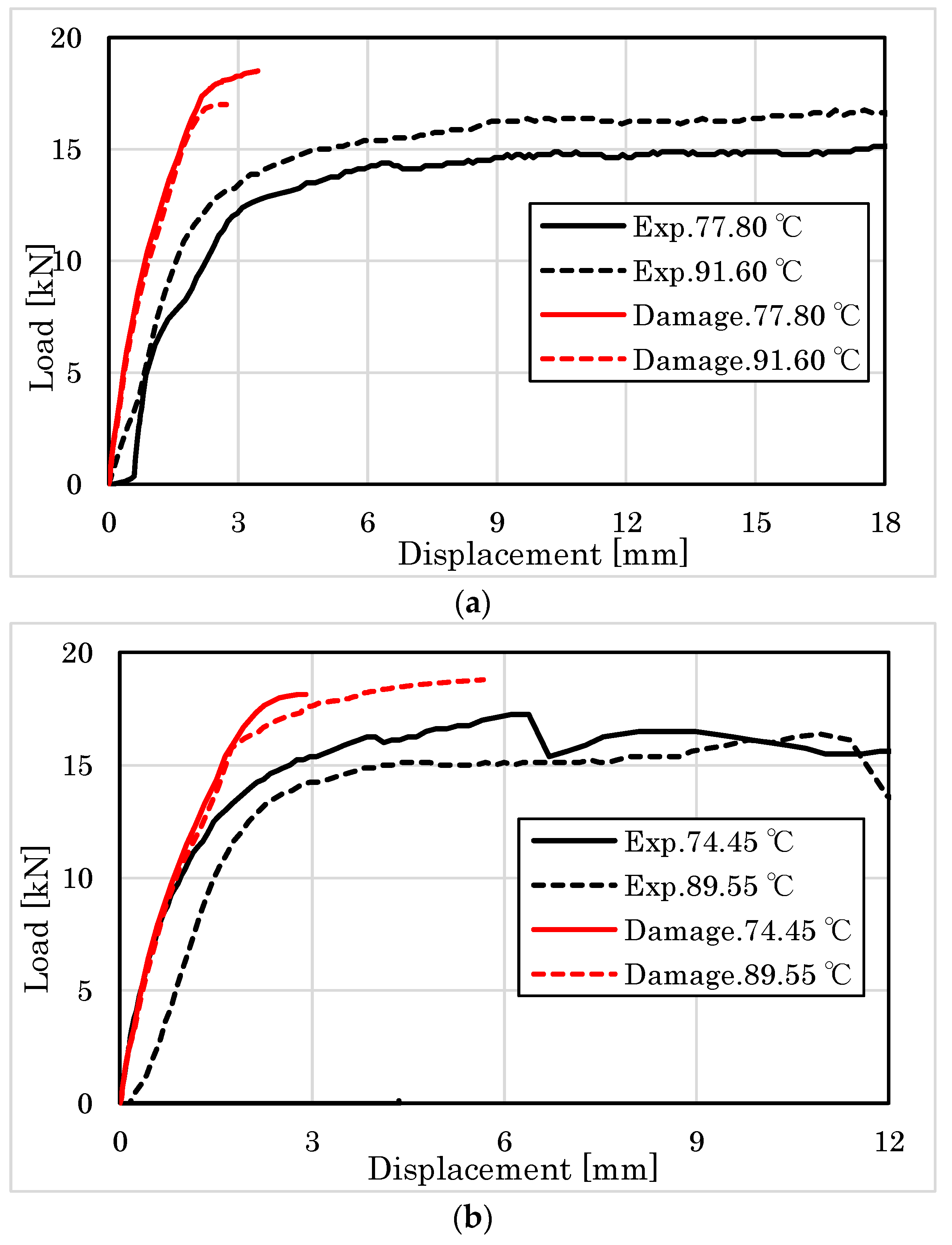
Figure 25.
Load–displacement relationship perpendicular at ambient temperature. (a) Cedar; (b) larch.
Figure 25.
Load–displacement relationship perpendicular at ambient temperature. (a) Cedar; (b) larch.
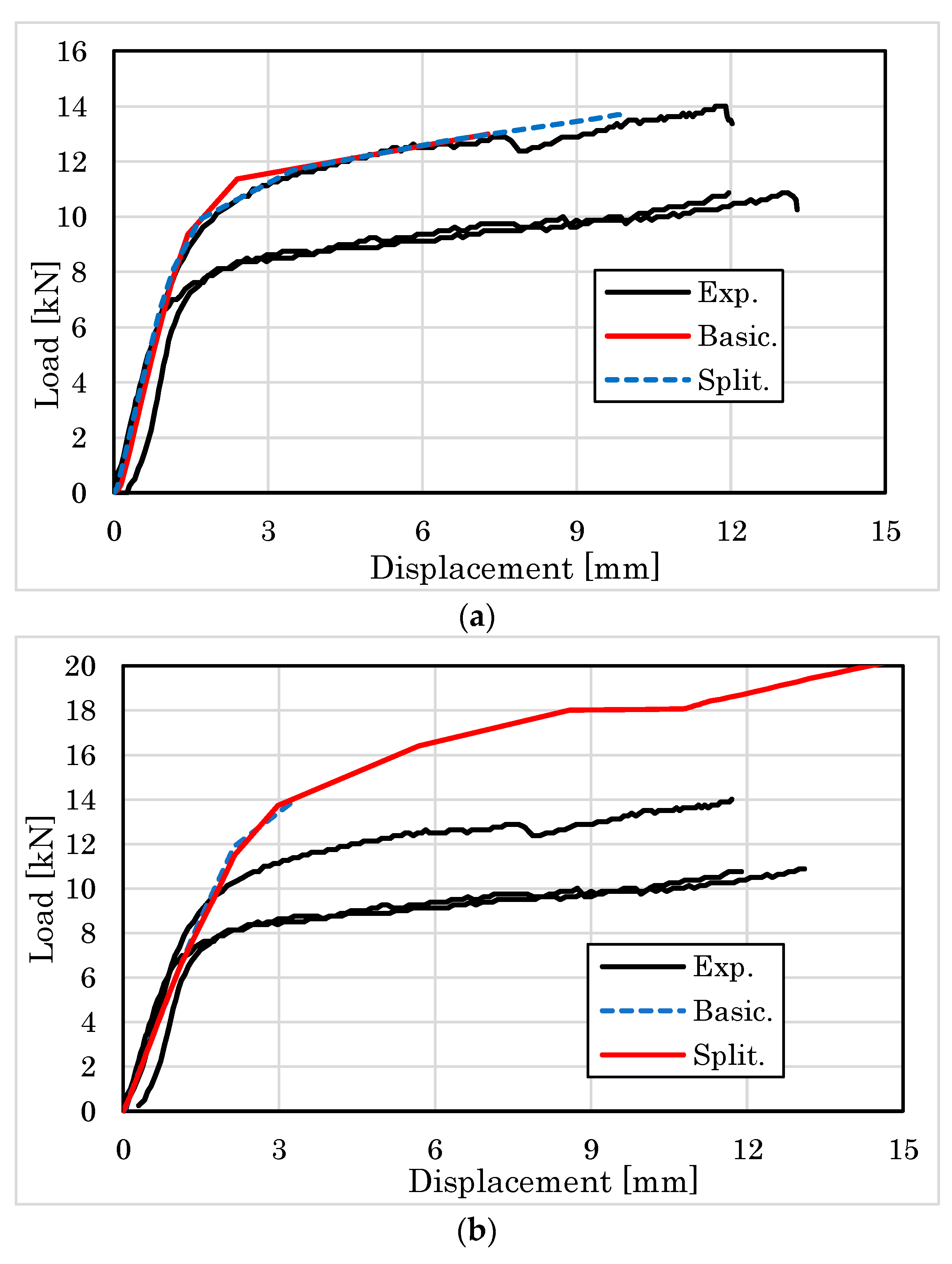
Figure 26.
Load–displacement relationship perpendicular at 60 °C heating temperature. (a) Cedar; (b) larch.
Figure 26.
Load–displacement relationship perpendicular at 60 °C heating temperature. (a) Cedar; (b) larch.
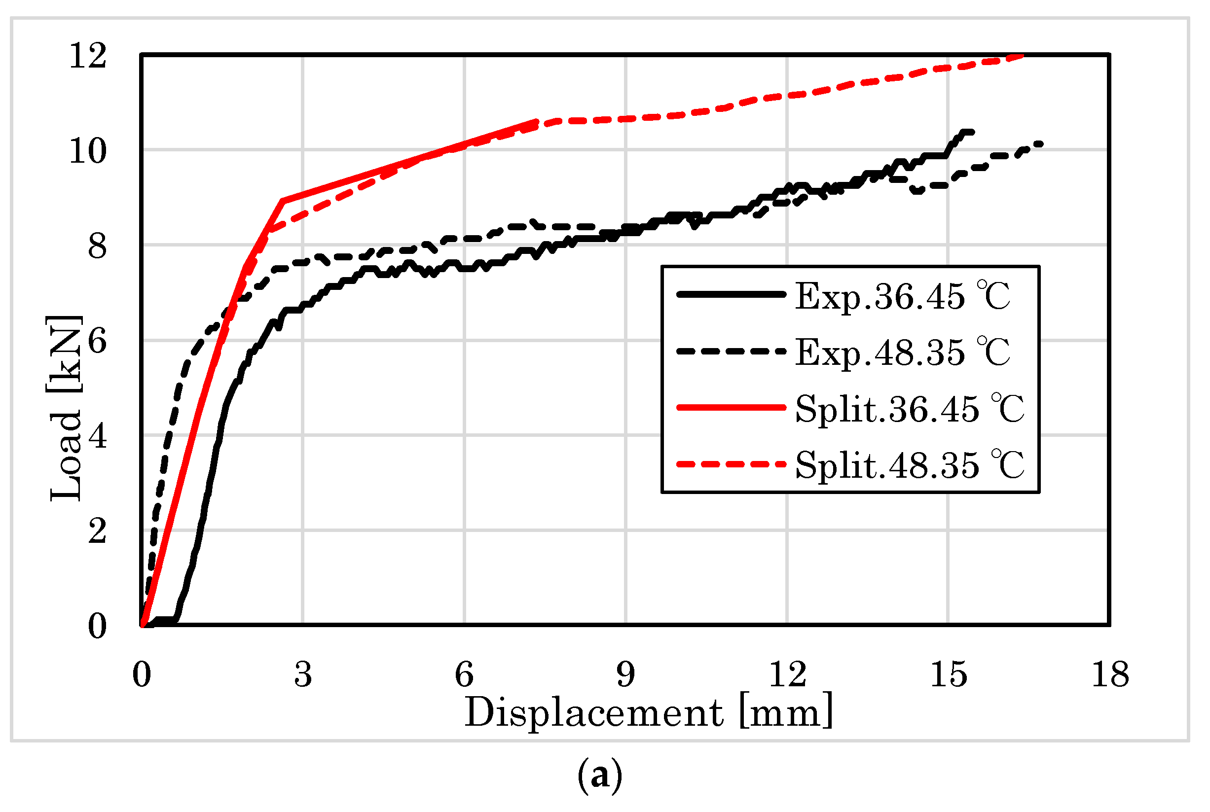
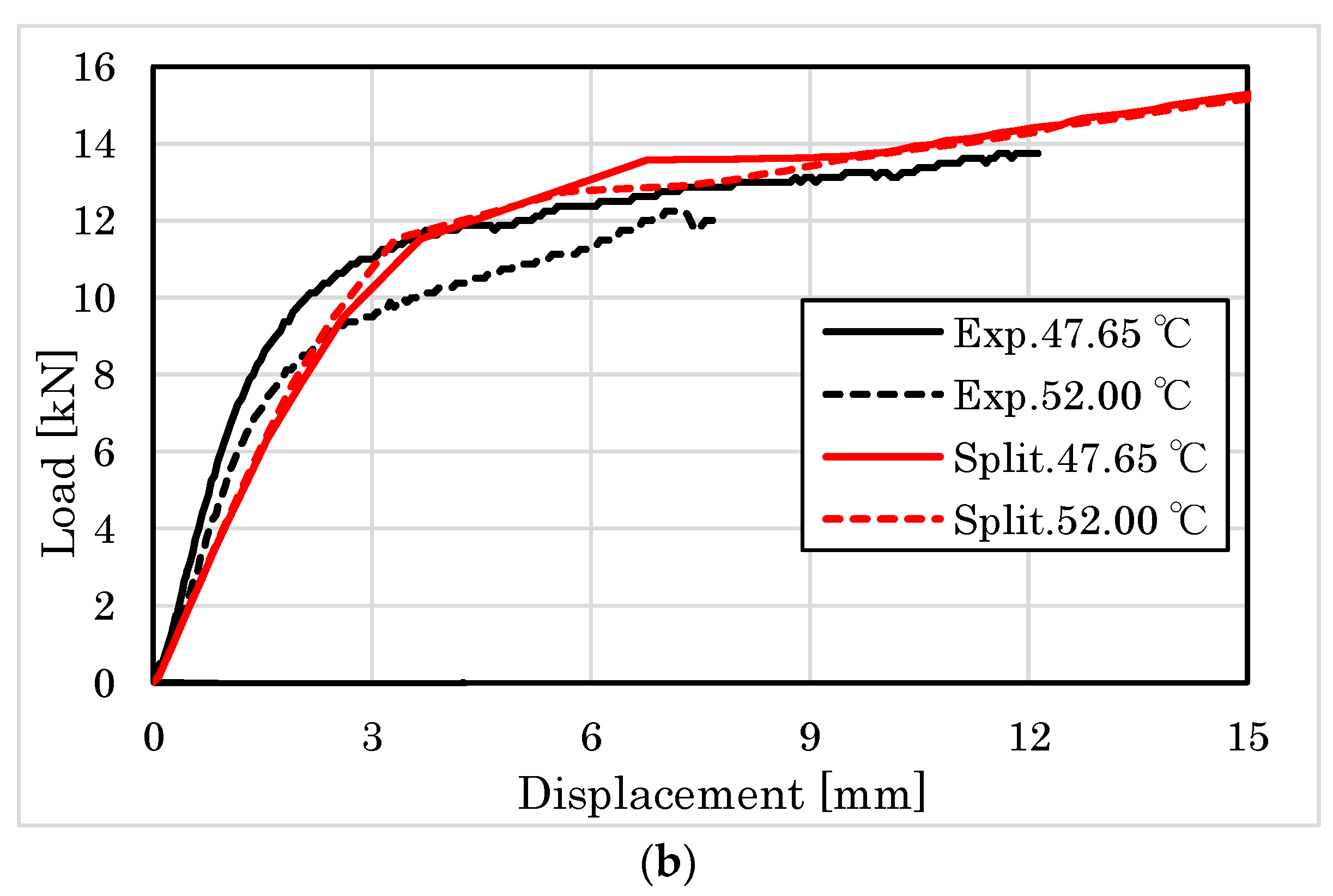
Figure 27.
Load–displacement relationship perpendicular at 100 °C heating temperature. (a) Cedar; (b) larch.
Figure 27.
Load–displacement relationship perpendicular at 100 °C heating temperature. (a) Cedar; (b) larch.
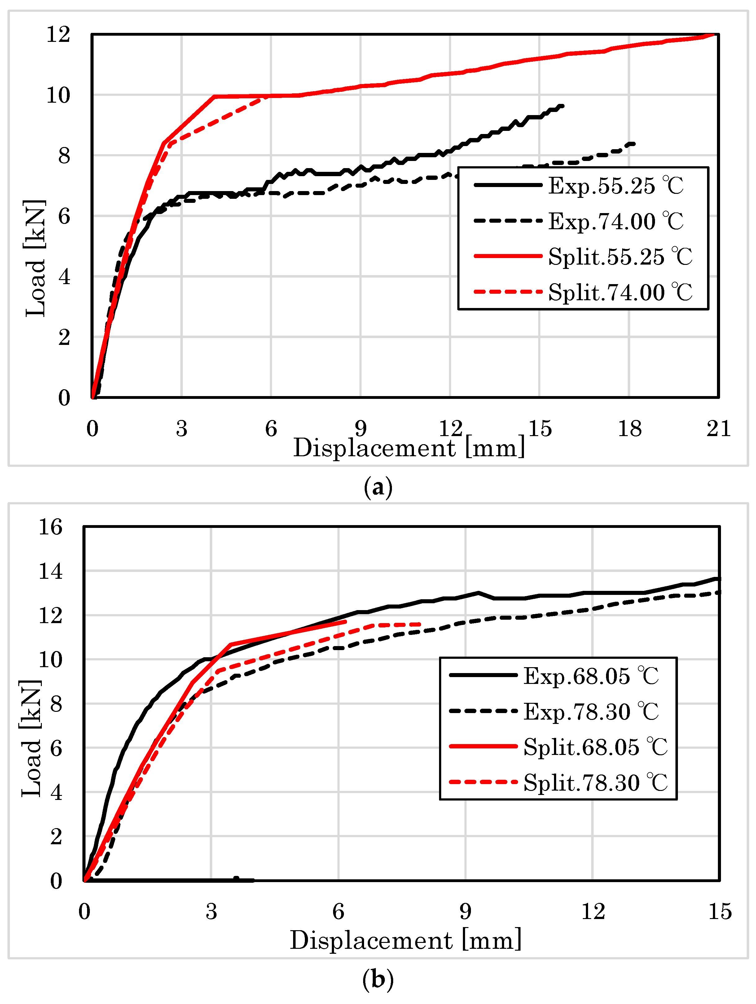
Figure 28.
Normal and shear stresses in one element at the center of the timber from the analysis (cedar ambient temperature perpendicular). (a) Load and stress–displacement relationship; (b) stress–displacement relationship.
Figure 28.
Normal and shear stresses in one element at the center of the timber from the analysis (cedar ambient temperature perpendicular). (a) Load and stress–displacement relationship; (b) stress–displacement relationship.
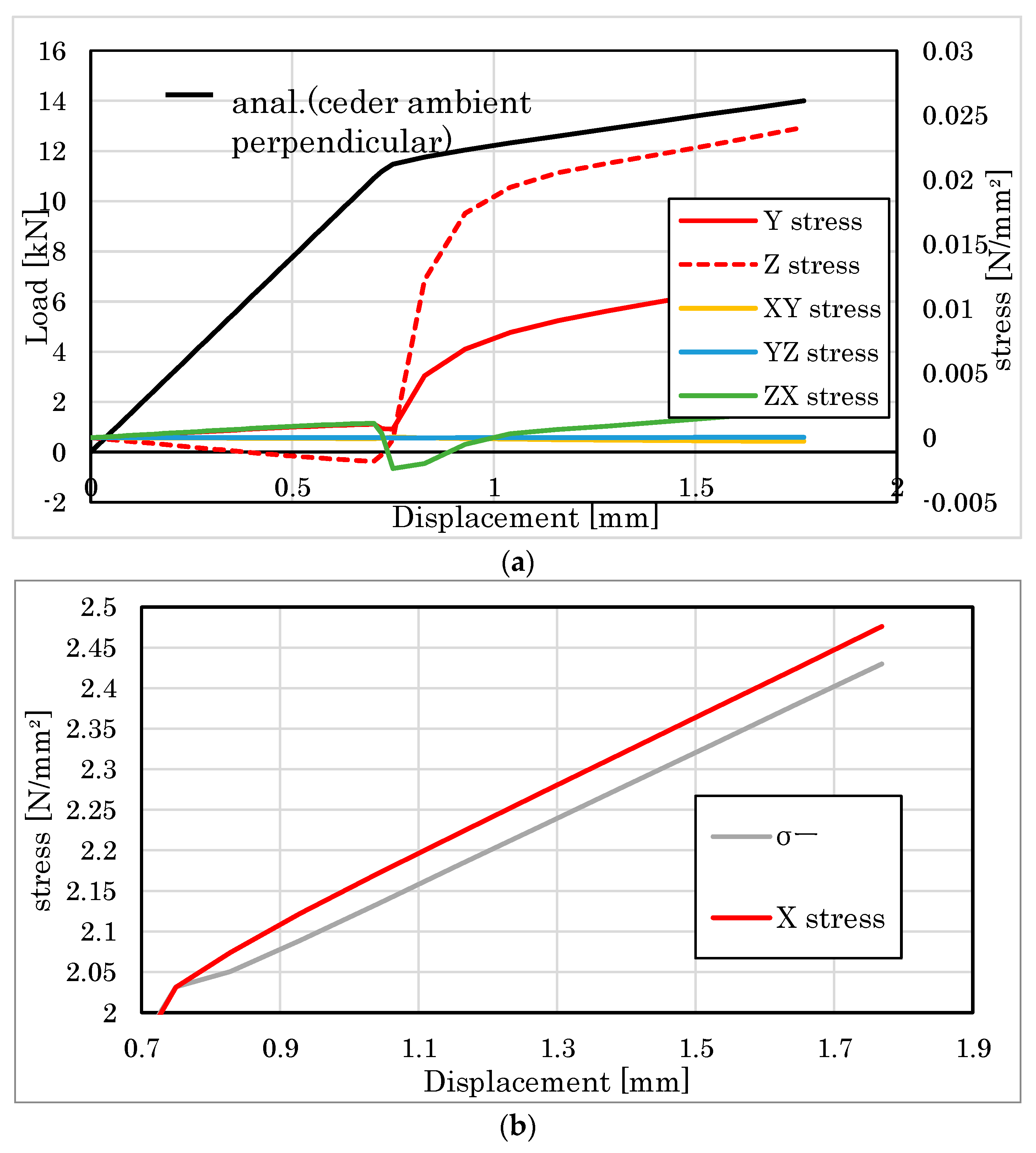
Figure 29.
Deformation diagram of parallel embedment tests at ambient temperature.
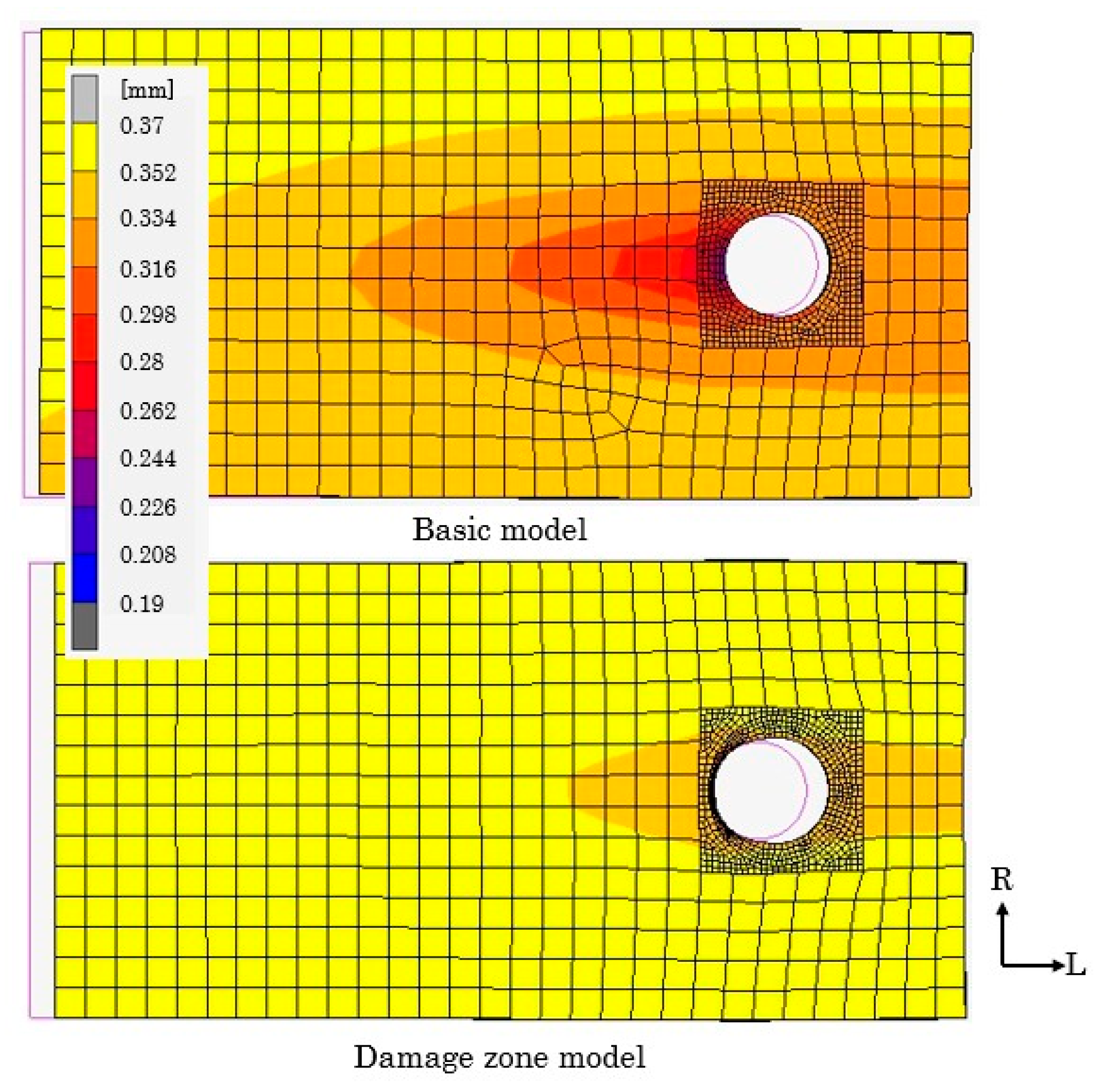
Figure 30.
Stress distribution of parallel embedment tests at ambient temperature.
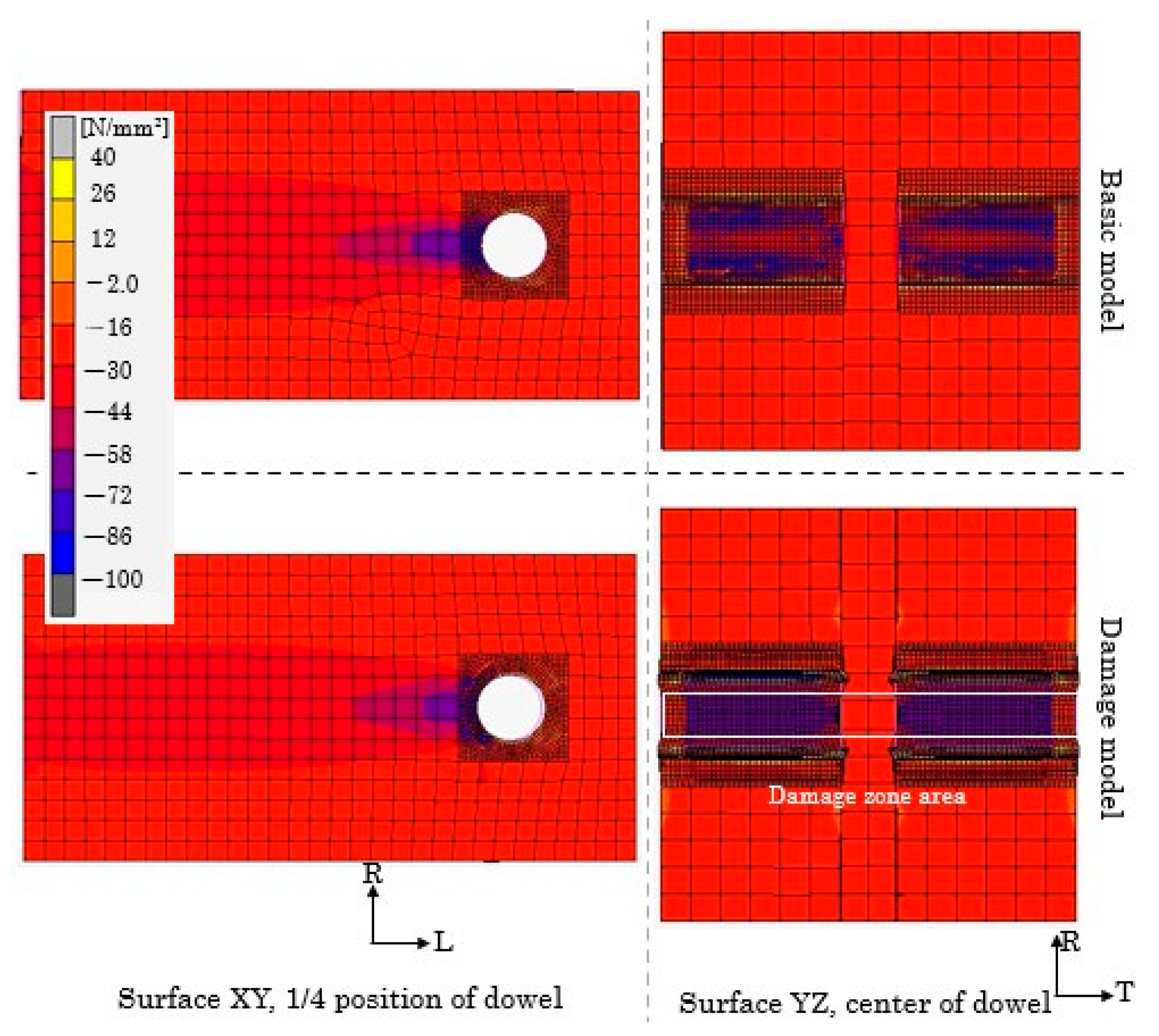
Figure 31.
Stress distribution of perpendicular embedment tests at ambient temperature.
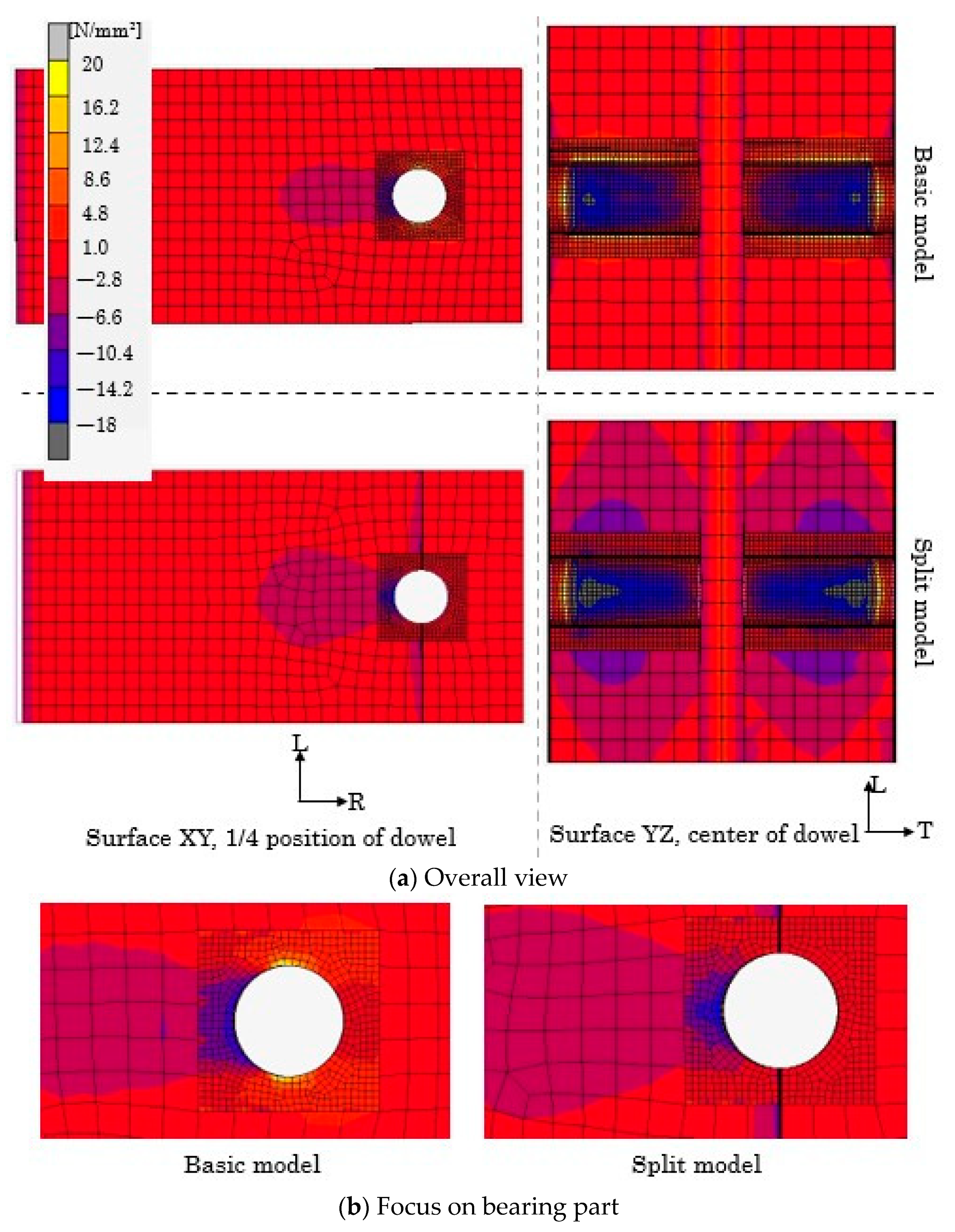
Figure 32.
Stress distribution of the split model at 100 °C.
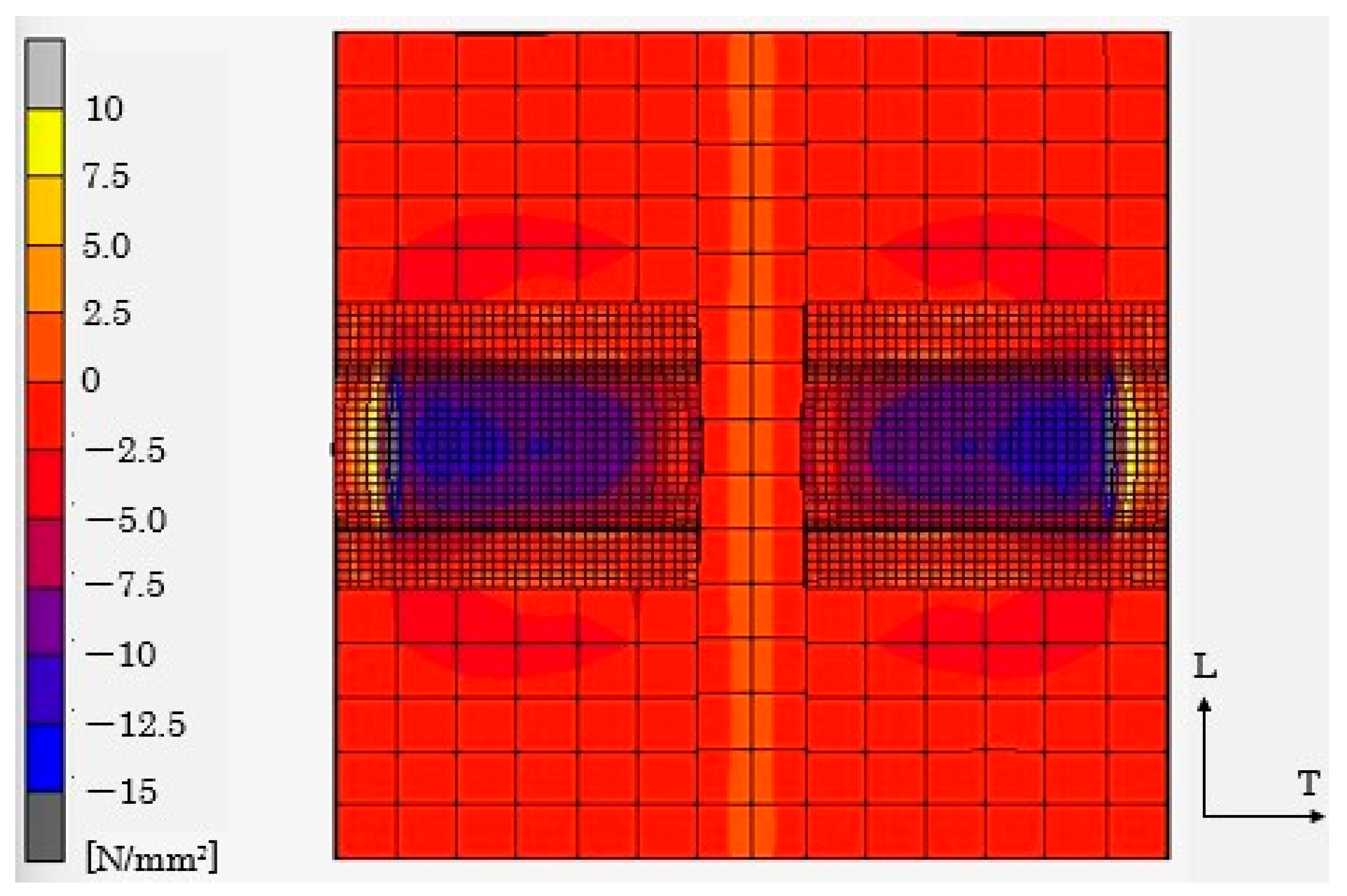
Figure 33.
Comparison of analysis result and fracture properties at ambient temperature. (a) Stress distribution on the XY-axis at maximum load; (b) fracture properties.
Figure 33.
Comparison of analysis result and fracture properties at ambient temperature. (a) Stress distribution on the XY-axis at maximum load; (b) fracture properties.
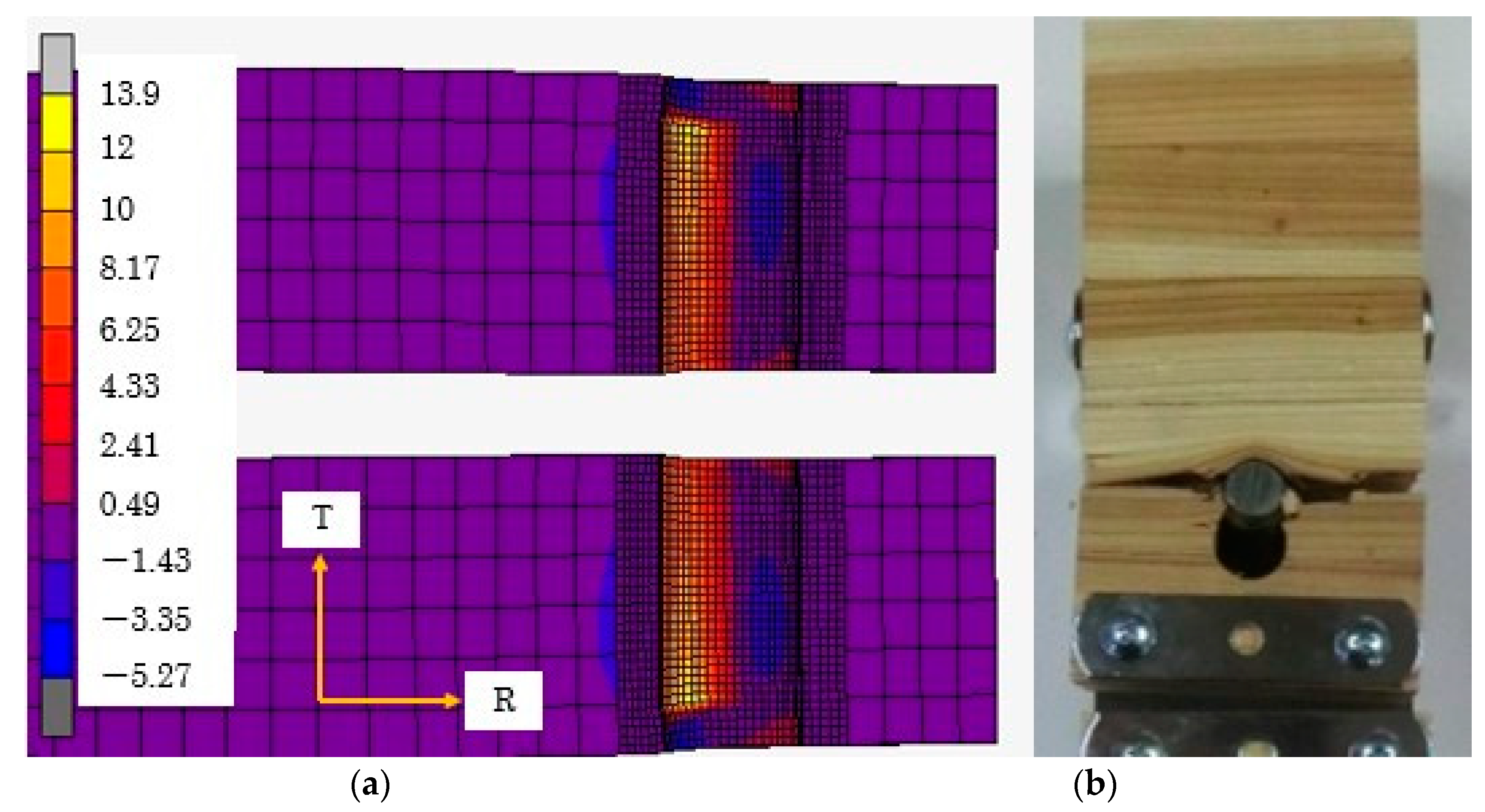
Table 1.
Heating conditions.
| Load Direction | Thermal Condition | Total | |||||
|---|---|---|---|---|---|---|---|
| Parallel to grain and perpendicular to grain | Ambient Temp. | 3 | 3 | ||||
| Constant temperatures (°C) | Heating time (hour) | ||||||
| 0.5 | 1 | 1.5 | 2 | 4 | |||
| 60 | - | 1 | - | 1 | 1 | 3 | |
| 100 | - | 1 | - | 1 | 1 | 3 | |
| 150 | - | 1 | - | 1 | 1 | 3 | |
| 200 | - | 1 | - | 1 | - | 2 | |
Table 2.
Result of temperature measurement.
| (a) Cedar | |||||
| Cedar | Constant Temperature (°C) | Heating Time (hour) | Temperature Measurement | ||
| ① | ② | Average | |||
| Parallel to grain | 60 | 1 | 44.1 | 53.4 | 48.75 |
| 2 | 54.8 | 58.3 | 56.55 | ||
| 100 | 1 | 69.7 | 85.9 | 77.8 | |
| 2 | 88.2 | 95 | 91.6 | ||
| 150 | 1 | 97.6 | 122.4 | 110 | |
| 2 | 112.3 | 136.1 | 124.2 | ||
| 200 | 1 | 105.3 | 163.8 | 134.55 | |
| 2 | 151.2 | 193.2 | 172.2 | ||
| Perpendicular to grain | 60 | 1 | 32.1 | 40.8 | 36.45 |
| 2 | 46.3 | 50.4 | 48.35 | ||
| 100 | 1 | 45.4 | 65.1 | 55.25 | |
| 2 | 68.4 | 79.6 | 74 | ||
| 150 | 1 | 71.5 | 94 | 82.75 | |
| 2 | 94.6 | 124.7 | 109.65 | ||
| 200 | 1 | 80.3 | 114.8 | 97.55 | |
| 2 | 125.7 | 175.3 | 150.5 | ||
| (b) Larch | |||||
| Larch | Constant temperature (°C) | Heating time (hour) | Temperature Measurement | ||
| ① | ② | average | |||
| Parallel to grain | 60 | 1 | 45.5 | 51.8 | 48.65 |
| 2 | 53.9 | 56.5 | 55.2 | ||
| 100 | 1 | 67 | 81.9 | 74.45 | |
| 2 | 86 | 93.1 | 89.55 | ||
| 150 | 1 | 92.5 | 110.9 | 101.7 | |
| 2 | 110.1 | 123.5 | 116.8 | ||
| 200 | 1 | 112.5 | 149.7 | 131.1 | |
| 2 | 131.9 | 169.5 | 150.7 | ||
| Perpendicular to grain | 60 | 1 | 45.7 | 49.6 | 47.65 |
| 2 | 49.9 | 54.1 | 52 | ||
| 100 | 1 | 64.4 | 71.7 | 68.05 | |
| 2 | 73.1 | 83.5 | 78.3 | ||
| 150 | 1 | 82 | 102.6 | 92.3 | |
| 2 | 97.5 | 119.1 | 108.3 | ||
| 200 | 1 | 100 | 130.6 | 115.3 | |
| 2 | 144.2 | 164.5 | 154.35 | ||
Table 3.
Young’s modulus and the yield stress.
| (a) Cedar | ||||
| Cedar | Constant Temperature (°C) | Heating Time (hour) | Young’s Modulus(N/mm2) | Yield Stress (N/mm2) |
| Parallel to grain | ambient | 7676.96 | 32.20 | |
| 60 | 1 | 6664.23 | 20.10 | |
| 2 | 7104.02 | 20.84 | ||
| 100 | 1 | 5913.00 | 18.51 | |
| 2 | 5914.02 | 16.04 | ||
| 150 | 1 | 4647.45 | 14.97 | |
| 2 | 4952.51 | 16.52 | ||
| 200 | 1 | 4165.56 | 14.22 | |
| 2 | 5062.71 | 16.69 | ||
| Perpendicular to grain | ambient | 413.25 | 2.03 | |
| 60 | 1 | 178.92 | 1.11 | |
| 2 | 264.19 | 2.11 | ||
| 100 | 1 | 173.57 | 1.46 | |
| 2 | 197.05 | 1.70 | ||
| 150 | 1 | 214.54 | 1.49 | |
| 2 | 210.17 | 1.43 | ||
| 200 | 1 | 170.94 | 1.34 | |
| 2 | 229.76 | 1.34 | ||
| (b) Larch | ||||
| Larch | Constant temperature (°C) | Heating time (hour) | Young’s modulus (N/mm2) | Yield stress (N/mm2) |
| Parallel to grain | ambient | 10,263.67 | 29.36 | |
| 60 | 1 | 10,013.69 | 28.38 | |
| 2 | 10,013.05 | 26.10 | ||
| 100 | 1 | 8077.27 | 20.67 | |
| 2 | 7822.52 | 18.00 | ||
| 150 | 1 | 8022.64 | 15.78 | |
| 2 | 6884.81 | 15.85 | ||
| 200 | 1 | 5968.15 | 21.39 | |
| 2 | 7487.83 | 22.87 | ||
| Perpendicular to grain | ambient | 298.86 | 2.67 | |
| 60 | 1 | 252.93 | 2.69 | |
| 2 | 220.10 | 2.15 | ||
| 100 | 1 | 133.42 | 1.77 | |
| 2 | 182.58 | 2.17 | ||
| 150 | 1 | 117.50 | 1.93 | |
| 2 | 148.65 | 2.10 | ||
| 200 | 1 | 106.60 | 1.90 | |
| 2 | 169.21 | 1.78 | ||
Table 5.
Material data of steel plate and dowels.
| Joining Hardware | Steel Plate | Drift Pin |
|---|---|---|
| JIS G 3101 | SS400 | SS400 |
| Specimen size (mm) | 9.0 × 75 × 200 | φ16 × 75 |
| Yield point (N/mm2) | 336 | 296 |
| Tensile strength (N/mm2) | 454 | 470 |
Table 6.
Material properties of the timber damage zone.
| Cedar | Larch | ||
|---|---|---|---|
| Young’s modulus (N/mm2) | EL | 138.19 | 181.02 |
| ER | 413.25 | 298.86 | |
| ET | 413.25 | 298.86 | |
| Poison’s ratios (–) | νLR | 0.0073 | 0.0136 |
| νRT | 0.90 | 0.93 | |
| νTL | 0.032 | 0.015 | |
| Share modulus (N/mm2) | GLR | 103.00 | 113.22 |
| GRT | 142.50 | 102.00 | |
| GTL | 102.74 | 113.52 | |
| Yield stress (N/mm2) | σyL | 32.20 | 29.73 |
| σyR | 2.03 | 2.67 | |
| σyT | 2.03 | 2.67 | |
| Damage Zone length (mm) | 3.7 | ||
Disclaimer/Publisher’s Note: The statements, opinions and data contained in all publications are solely those of the individual author(s) and contributor(s) and not of MDPI and/or the editor(s). MDPI and/or the editor(s) disclaim responsibility for any injury to people or property resulting from any ideas, methods, instructions or products referred to in the content. |
© 2023 by the authors. Licensee MDPI, Basel, Switzerland. This article is an open access article distributed under the terms and conditions of the Creative Commons Attribution (CC BY) license (https://creativecommons.org/licenses/by/4.0/).
Share and Cite
MDPI and ACS Style
Kawai, Y.; Totsuka, M.; Hirashima, T. Elastoplastic Analysis of Timber Connections with Dowel-Type Fasteners at Ambient and High Temperatures. Forests 2023, 14, 373. https://doi.org/10.3390/f14020373
AMA Style
Kawai Y, Totsuka M, Hirashima T. Elastoplastic Analysis of Timber Connections with Dowel-Type Fasteners at Ambient and High Temperatures. Forests. 2023; 14(2):373. https://doi.org/10.3390/f14020373
Chicago/Turabian StyleKawai, Yuga, Marina Totsuka, and Takeo Hirashima. 2023. "Elastoplastic Analysis of Timber Connections with Dowel-Type Fasteners at Ambient and High Temperatures" Forests 14, no. 2: 373. https://doi.org/10.3390/f14020373
Note that from the first issue of 2016, this journal uses article numbers instead of page numbers. See further details here.