Effects of Climate on Stand-Level Biomass for Larch Plantations in Heilongjiang Province, Northeast China


1
Department of Forest Management, School of Forestry, Northeast Forestry University, Harbin 150040, China
2
Key Laboratory of Sustainable Forest Ecosystem Management-Ministry of Education, School of Forestry, Northeast Forestry University, Harbin 150040, China
*
Authors to whom correspondence should be addressed.
†
These authors contributed equally to this work.
Forests 2023, 14(4), 820; https://doi.org/10.3390/f14040820
Submission received: 13 January 2023
/
Revised: 27 March 2023
/
Accepted: 13 April 2023
/
Published: 17 April 2023
(This article belongs to the Section Forest Inventory, Modeling and Remote Sensing)
Abstract
:Climate change affects forest resource availability, growing season length, and thus forest biomass accumulation. However, only a limited number of studies have been conducted on forest biomass management based on climate effects, particularly at the stand-level. Thus, an allometric biomass equation based on conventional and climate-based stand biomass models, was developed and compared for larch trees (Larix spp.). A total of 160 experimental plots of larch plantations have been collected in Heilongjiang Province, Northeast China. In this study, we developed four types of additive model systems for stand-level biomass: two types of the stand-level biomass basic models (M-1 and M-2) with stand variables (stand basal area (BA) and stand mean height (Hm)) as the predictors, and two types of the proposed stand-level biomass climate-based models (M-3 and M-4) with stand variables (BA and Hm) and climatic variables (mean annual temperature (MAT) and annual precipitation (AP)) as the predictors. Accordingly, this study evaluated the effects of climatic variables (MAT and AP) and stand variables (BA and Hm) on the model’s performance. Model fitting and validation results revealed that the climatic variables significantly improved the model performance of the fitted equation by increasing the coefficient of determination (R2) values and reducing the root mean square error (RMSE) values. A higher R2 and a lower RMSE were consistently generated by M-2 and M-4, whereas M-1 and M-3 consistently generated a lower R2 and a higher RMSE. We found that the proposed stand-level biomass climate-based model type 4 (M-4) performed better than the other models and slightly better than in previous studies of climate-sensitive models. This study provided an additional and beneficial method of analyzing climate effects on stand-level biomass estimation.
1. Introduction
Since the 1950s, global climate change has continuously affected human populations and various ecosystems on earth. While climate change is gradually impacting the world, natural disasters and extreme weather are also caused by it. The effects of these changes have been felt by wildlife and human life [1,2,3]. During the past few years, the global intergovernmental community has attempted to mitigate the effects of rising carbon emissions and limit the global temperature increase to 1.5 °C [2]. To address these environmental issues, established forest plantations through planted forests (i.e., afforestation and reforestation) have become an important tool for carbon sequestration and climate change mitigation [4,5,6,7,8]. In light of this, the United Nations Framework Convention on Climate Change (UNFCCC) has committed to reducing emissions from deforestation and forest degradation. Forest ecosystems are the major terrestrial carbon sinks, storing around 80% and 40% of terrestrial above-ground and below-ground carbon, respectively [9,10,11]. The majority of studies to date have paid more attention to estimating forest biomass rather than estimating carbon storage, due to the fact that forest carbon concentrations are estimated to be approximately constant for tree or stand components (around 50%) [12]. In addition, forest biomass estimation with high accuracy has become fundamental for sustainable forest management [12]; it also has been of interest to forest researchers throughout the world in recent decades, including American and European [13,14,15,16], Asian and Oceanian [17,18,19,20], and African [21,22,23].
A forest biomass modeling process can be conducted using a variety of procedures, and the decision to use one method over another depends on the availability of data. On a local scale, one of the most widely used approaches is that of scaling-up, which requires individual tree data sets, such as diameter at breast height (DBH), and height. It is possible to predict biomass at stand-level using the summation of individual trees’ predicted biomass model quantities. This allows forest managers and decision-makers to be more efficient in predicting biomass in terms of time and cost. Individual tree availability data, however, are rarely available on a large scale. As an alternative, it has been suggested that forest inventories be connected [24,25]. By easily measuring stand variables such as stand basal area, stand average height, and stand quadratic mean diameter at breast height, the study shows stand biomass benefits for forest biomass estimation [12,26]. According to Parresol [15], stand biomass per hectare was calculated by aggregating a number of trees. The model was then developed by predicting those variables within a stand. As an additional benefit, stand variables reduce the complexity of error propagation processes at various spatial scales [27]. Therefore, it is important to aim to predict the forest biomass at a stand-level by reducing the number of samples in forest measurement, in order to improve reliability and time-cost efficiency.
The fitting process of forest biomass parameter estimation can be estimated using linear regression or nonlinear regression, with nonlinear regression being highly effective in these estimations [28,29]. The flexibility and generality of nonlinear seemingly unrelated regression (NSUR) that was proposed by Parresol [16], make it a widely used method to estimate parameters in nonlinear stand biomass models [12]. Similar to tree biomass models, stand biomass models often encounter heteroscedasticity, and the weighting function has been used to address heteroscedasticity for each equation [12,30].
In recent years, due to the consequences of climate change, the development of biomass models has been characterized by the importance of incorporating climatic variables into the models [11,31,32]. Nonetheless, most studies on biomass modeling under climate effects focus only on individual trees in many countries and species. For example, in China, Fu et al. [33] developed an allometric equation for Masson pine (Pinus massoniana Lamb.), and Gao et al. [31] and Zeng et al. [34] developed an allometric equation for larch (Larix spp.); in South America, Laclau [13] studied biomass and carbon sequestration of ponderosa pine (Pinus ponderosa (Dougl.) Laws) and native cypress (Austrocedrus chilensis (Don) Flor. et Boutl.); in Germany, Krug [35] studied biomass and carbon dioxide sequestration of European beech (Fagus sylvatica L.); and in Europe, Forrester et al. [36] developed biomass and leaf area allometric equations for many European tree species, although only a few studies examined stand-level biomass. Moreover, it is critical to understand forest biomass’ role in carbon stocks and mitigating climate change. Unfortunately, a limited number of studies have examined the impact of climate change on stand biomass [37]. To this end, this study hypothesizes that incorporating climate variables into stand biomass models can reduce the uncertainty associated with forest biomass and carbon storage.
Larch (Larix spp.) is an important economically and ecologically valuable tree species in China, being a fast-growing coniferous tree species planted for many timber industries [34,38]. The larch tree is also highly resistant to cold conditions, making it one of the most fundamental components of the Northeast China forest ecosystem for establishing national reserve forests [38,39,40]. In China, larch plantations cover approximately 3.14 million hectares, making them the 4th most abundant tree species, which is critical in sequestering atmospheric carbon [38,41,42]. As the largest forest area in China, Heilongjiang province, with a forest coverage of 46%, has a fundamental role in China’s forest ecosystem [43]. Studies have demonstrated the importance of estimating biomass and carbon to mitigate climate change’s effects [6,44,45]. However, only a limited number of studies examine the effects of climate variables on stand-level biomass estimation [12,24,41,46,47]. Moreover, the response of larch species studies to the climate in Northeast China is still challenging [39,48,49]. Thus, this study examined the stand-level biomass model and its correlation with climate variables’ effects on larch plantations in Heilongjiang Province, Northeast China.
The objectives of this study were: (1) to develop four types of additive model systems for stand-level biomass—two basic models (M-1, M-2) and two proposed stand-level biomass climate-based models (M-3, M-4)—for larch plantations in Heilongjiang Province, Northeast China; (2) to evaluate the accuracy of model fitting and model performance on different additive methods (M-1, M-2, M-3, and M-4); and (3) to determine the effect of climatic variables on stand-level biomass estimations.
2. Materials and Methods
2.1. Study Area
This study selected larch plantation forest plots in different locations in Heilongjiang Province, Northeast China (44°04′–50°69′ N and 122°63′–132°78′ E). The province has a 454,000 km2 total land area and has been designated as one of the national critical forest and grass resource distribution areas, with around 20.8 million hectares of forest (approximately 45.8% of the total land area of the province) [43,50]. The province’s elevation is approximately 36% higher than 300 m, formed by 4 major mountain ranges. This study area is located in the northern temperate continent, in a monsoon climate zone between temperate and frigid zones, and the annual average temperatures ranges from −5.0 °C to 5.0 °C, while the annual average precipitation ranges from 400 mm to 670 mm. In Heilongjiang, the forest soil type is predominantly dark brown soil. Heilongjiang province has several vegetation types, including cold temperate coniferous forests, temperate coniferous forests, and broad-leaf mixed forests [43,51,52].
The study areas were distributed north to south and west to east of Heilongjiang province. Larch trees are classified as members of the Pinaceae family and are part of the genus Larix. Typically, they are found in cold climates with plenty of moisture sites, a type of high-productivity coniferous timber production in China that is both ecologically and economically beneficial. High commercial value, better quality timber, and straight stem, are characteristics of the larch. China’s ninth National Forest Inventory reported that Larix gmelinii plantations are among the most popular larch species, and are a top ten tree species in terms of plantation area. There are 2.51 million ha of Larix gmelinii plantations in China, with a stock volume of 238 million m3 [53]. Larch is also the most important species group in the northeastern Chinese forest ecosystems, occupying approximately 25% of the forest area [39].
2.2. Data Collection
The authors identified and selected 160 experimental sampling plots of larch plantations that ranged in size from 0.09 to 0.1 ha (Table 1). We used a random sample of temporary plots in the site. The larch is the dominant tree species, and the volume of larch is ≥ 65% in each sample plot, representing a pure plantation forest by Li [49,54]. The slope of the plots ranged from 5 to 25°. The stand density was 333 to 1778 per hectare. Most plots were pure larch forest and others contained small amounts of other tree species. The biomass data was acquired from 2005 to 2019. All trees with diameters at breast height (DBH) greater than 5 cm were examined throughout the sample plot. The measurement information of individual tree variables included DBH (1.3 m above the ground), whole tree height, the first living branch height, and the position of each tree. The DBH measurement accuracy is 0.1 cm, and the other variables’ measurement accuracies are each 0.1 m. We also recorded the key stand variables of stand mean height (Hm, m) and stand age (Age, year). Other stand variables, such as stand basal area (BA, m2/ha), stand quadratic mean diameter at breast height (Dg, cm), and stand density (N, trees/ha), were also obtained. In this study, Age was the average age of the larch tree species in the sample plot, and Hm was the mean of tree height in the plot. The data regarding stand variables are shown in Table 1.
2.3. Stand Biomass Calculation
The biomass of trees was determined using species-specific biomass models, which were developed by forestry researchers [55,56] and rely on diameter at breast height. These models include total and component (root, stem, branch, and needle) biomass estimates for major tree species in Heilongjiang Province, Northeast China. Then, individual biomass components (tree root, stem, branch, and needle) and total biomass (the sum of root, stem, branch, and needle), were calculated. The procedure for obtaining plot biomass is to sum all the live biomass trees within each sample plot, and convert it into stand biomass per hectare (Equation (1)).
where Bi (i = r, s, b, n, t) represents the stand root, stem, branch, needle, and total biomass (Mg·ha−1); bij represents the biomass of the ith component of the jth tree in a sample plot (Mg); j = 1 … n represents the number of trees in each sample plot; and A represents the sample plot area (ha). The stand biomass summary statistics in this study are presented in Table 1.
2.4. Climate Data
Throughout this study, climate data were obtained from the WorldClim version 2.1 climate dataset (https://worldclim.org/, accessed on 27 September 2021); there are 19 bioclimatic variables that represent average values. The data include monthly climate data for minimum, mean, and maximum temperatures, precipitation, solar radiation, and wind speed, among other variables [32]. Following the preliminary data analysis, we selected mean annual temperature (MAT) and annual precipitation (AP) to represent annual trends in this study [57]. Moreover, the preliminary data analysis showed MAT and AP performing better in having robust relationships with stand biomass variables than did other climate variables (Figure 1). Therefore, in this study, only MAT and AP were used. The previous study in China also obtained climate data from WorldClim and used it as the study baseline data [33,41,58,59]. A statistical summary of the climatic variables in this study are presented in Table 1.
2.5. Stand Biomass Model Development
In this study, the general model system forms were developed using nonlinear seemingly unrelated regression (NSUR) proposed by Parresol [16]. NSUR is a widely used parameter estimating technique, since it may guarantee additivity by simultaneously fitting the system and considering the limitations of linear correlation between components. The flexibility and generality of NSUR allow the component models to use different independent variables and different weight functions for heteroscedasticity in the system, resulting in a low variance for the total biomass [46]. On another note, NSUR has become more flexible in adding subtotal biomass, and Parresol [16] recommends introducing one or more constraints to the concurrent systems, such as the crown or aboveground biomass. Due to its simplicity and efficiency, NSUR is used extensively in crown width models, individual tree models, and stand biomass models [8,12,49,60].
The preliminary visual has plotted the stand biomass components (i.e., root, stem, branch, and foliage) against the basal area (BA), stand mean height (Hm), mean annual temperature (MAT), and annual precipitation (AP) (Figure 1), which indicates that the relationship between the stand biomass components and the basal area is more robust than other variables. Several previous studies have also employed stand basal area to predict stand-level biomass, i.e., Castedo-Dorado et al. [27] and Bi et al. [24] demonstrated a correlation between stand biomass (component and total biomass) and the basal area (BA) [12,61]. Following the general model formed by Parresol [15] and the nonlinear model’s system of biomass additivity proposed by Parresol [16], the inventory variables were used to adjust these relations, and two forms of biomass additivity models (stand basal area and stand variable-based models with an additive error term) for larch plantations were examined on the following model form (Equations (2) and (3)).
where Bi is the stand biomass (Mg·ha−1); BA is the basal area (m2·ha−1); Xn is the candidate stand variable, where BA and Hm represent the stand basal area (m2·ha−1) and stand mean height (m), respectively; (i = 0, 1, …, n) denotes the parameters to be estimated; and is the error term.
2.5.1. Basic Model
To ensure compatibility between the total biomass and the summation of each component biomass, we adopted an additive model system with five-term correlation among equations [24]. This study thus developed four types of additive model systems for stand-level biomass: two types of basic models and two types of climate-based models. The two types of basic models are: model type 1 (M-1), using simultaneous equations based on Equation (2), with the stand basal area as the only predictor (Equation (4)); and model type 2 (M-2), using simultaneous equations based on Equation (3), with the stand basal area and the stand mean height as predictors (Equation (5)).
Model type 1:
Model type 2:
where Bi (i = r, s, b, n, t) denotes the stand root, stem, branch, needle, and total biomass (t·ha−1); (i = 1, 2, 3, 4) are the model parameters to be estimated in the fitting process, (i = r, s, b, n, t) denotes the stand root, stem, branch, needle, and total biomass error term; and BA and Hm are the stand basal area (m2·ha−1) and stand mean height (m), respectively.
2.5.2. Stand-Level Biomass Climate-Based Model
Our study proposed the incorporation of climatic variables into a stand biomass model using the reparameterization method [62]. Based on the preliminary analysis of various stand biomass and climatic variables, it was determined that BA, Hm, MAT, and AP outperformed various statistical indicators. In order to model those two stand variables (BA and Hm) and those two climatic variables (MAT and AP), we selected them as candidate variables for the model. Further, we proposed a stand-level biomass climate-based model: model type 3 (M-3), using simultaneous equations based on Equation (4), with the stand variable (only stand basal area) and climatic variables as the predictors (Equation (6)); and model type 4 (M-4), using simultaneous equations based on Equation (5), with the multiple stand variables (stand basal area and stand mean height) and climatic variables as the predictors (Equation (7)).
Model type 3:
Model type 4:
where Bi (i = r, s, b, n, t) denotes the stand root, stem, branch, needle, and total biomass (Mg·ha−1); (i = 1, 2, 3, 4) are the model parameters to be estimated in the fitting process; (i = r, s, b, n, t) denotes the stand root, stem, branch, needle, and total biomass error term; BA and Hm are the stand basal area (m2·ha−1) and stand mean height (m); and MAT and AP are the mean annual temperature (°C) and annual precipitation (mm), respectively.
2.6. Weighting Function to Overcome Heteroscedasticity
Forest modeling is often faced with heteroscedasticity [15,16,63,64], which is reflected by inconsistent residuals. A particular configuration is often found in the residuals of base model estimates during the stand biomass modeling process [12]. The increase or decrease in the residuals may simultaneously increase the predicted value, for instance. Therefore, in this study, we fixed the heteroscedasticity of the residuals in each stand-level biomass model and stand variable by applying the weighting function [65]. In the first step, the stand total and components models were fitted by nonlinear seemingly unrelated regression (NSUR) to obtain the residual variance with heteroscedasticity [16,66]. We modeled the residual variance using the power function and the explanatory variables [49]. Thus, we assume as follows:
where is the residuals for the i model; i is the root, stem, branch, needle, and total; is the variance of residuals; – are parameters to be estimated; and x1–xn are explanatory variables.
In the second step, the unweighted residual variance with heteroscedasticity from the first step was squared while simultaneously transforming the explanatory variables by the natural logarithm (ln), and the stepwise regression was also used in the following formula:
where is the unweighted residuals; and the other symbols are as they have been previously defined in this paper.
In the third step, we estimated the Equation (9) using stepwise regression, and the weighting function for heteroscedasticity was for the ith equation. In the last step (the fourth step), fixing the weighting function, we were fitted again the equation system as in the second step, using an NSUR through SAS/ETS MODEL Procedure [67], and we added the weighting function to the procedure, thus specified as (where is the residual of the i model) [30,68].
2.7. Statistical Analysis and Model Evaluation
We used the goodness-of-fit to measure the fitting of the basic and the proposed stand-level climate-based models by utilizing two commonly used statistical indices, the coefficient of determination () and the root mean square error (RMSE). In addition, the leave-one-out cross-validation method (LOOCV) was used to validate the model’s performance. The method process is as follows: First, we considered one sample from the entire data set at a time, and the other samples were elaborate in the model fitting. The validation of the one sample obtained the model parameters. Second, we repeated the first step only once each sample was taken, using all-but-one observation ( − 1, is the number of samples) [69]. Third, after the second process, we calculated the coefficient of determination (), the root mean square error (RMSE), the root mean square prediction error (RMSPE), the mean absolute error (MAE), the root mean square prediction error (MAPE), and the mean prediction error (MPE), to evaluate the performances of the basic and stand-level biomass climate-based models. The higher the values of , the lesser the RMSE, RMSPE, MAE, MAPE, and MPE, indicate the accuracy of the model’s predictions. This study performed the data analyses using the SAS 9.4 version [67], and the graphical analyses using the R programming language [70]. These statistical analyses and model evaluations are as shown in Equations (10)–(15).
where is observed values, is estimated values, is the mean value of samples, and is the number of samples.
3. Results
3.1. Model Fitting
Parameter estimates were highly significant among the 4 types of additive model systems for stand-level biomass (M-1, M-2, M-3, and M-4) (Table 2), p < 0.001; all parameters were statistically significant. Standard errors ranged from 0.0011 to 0.1085. Multicollinearity was tested using a variance inflation factor (VIF) during the modeling process, and the VIF for all models was found to be less than five. The entire dataset of larch was employed for fitting the stand total and its four component biomasses (root, stem, branch, and needle).
Furthermore, the model parameters (ai, bi, ci, di, fi) that determine the power of the base predictors (BA, Hm, MAT, and AP), varied from positive to negative according to the base predictor. There was a relationship between the model parameters of the predictors and the biomass components (Table 2). In the basic models (M-1 and M-2), which only employ BA and Hm as the base predictors, all power factors of BA and Hm were positive. Meanwhile, incorporating climatic variables (MAT and AP) caused several changes in the parameters of stand-level biomass climate-based models (M-3 and M-4), which showed positive and negative significant nonlinear relations between the climatic factors and the stand biomass. There were positive powers of BA in M-3, while positive powers of MAT were found in the stand root, stem, and needle biomass, but negative powers of MAT were found in the stand branch biomass. Based on these results, it was found that for the same BA, the stand root, stem, and needle biomass increased, but the stand needle biomass decreased with an increase in MAT. In addition, the powers of AP were negative in the stand root biomass, which indicates that the stand root biomass decreased as AP increased. The powers of BA, Hm, and AP in M-4 were all positive, and the powers of MAT were positive in the stand stem biomass but negative in the stand root, branch, and needle biomass. According to these results, stand stem biomass increased for the same BA, Hm, and AP, but the stand root, branch, and needle biomass decreased with increasing MAT.
The climate variables (MAT and AP) and stand variables (BA and Hm) were applied to weight function, a stepwise regression process was implemented to fulfill backward elimination and forward selection, and the results indicated that the climate variables were not significant and that the Hm was partially significant (Table 3). Therefore, we used only the weight functions associated with BA. The R2 for the stand-level biomass climate-based model (M-4) generally ranged from 0.9479 to 0.9874, the model with the basal area as the predictor and climatic variables as the predictor exponential function (M-3) ranged from 0.9438 to 0.9743, the model with the basal area and stand average height as the predictors (M-2) ranged from 0.9349 to 0.9844, and the model with the basal area as the only predictor (M-1) ranged between 0.9322 and 0.9644 (Table 3). In general, the goodness-of-fit analysis showed that the proposed model (M-4) performed better than the basic model (M-2), and the model using BA and Hm as predictors (M-2) performed better than the model using BA only as a predictor variable (M-1). Meanwhile, M-2 performed better than M-3 due to the Hm effects. A model with multiple variables (BA, Hm, and climatic variables) performed better than other models. However, climatic variables with BA but without Hm as variables, performed lower than climatic variables with both BA and Hm as variables. There was a consistently higher RMSE yielded by M-1 and M-3, while lower RMSE values were generated by M-2 and M-4, with M-1 yielding the highest RMSE and M-4 yielding the lowest RMSE. Additionally, the RMSE values were highest for the stand total, stem, and root biomass, and lowest for the stand branch and needle biomass.
The inclusion of MAT and AP enhanced the stand-level biomass climate-based models (M-3 and M-4), especially the stand root biomass. Overall, when M-1 and M-3 are compared using the total of all biomass components (root, stem, branch, and needle) in the stand, the R2 increases from 0.97% to 2.71%, and the RMSE decreases from 8.95% to 26.32%. When M-2 and M-4 are compared using the total of all biomass components (root, stem, branch, and needle) in the stand, the R2 increases from 0.30% to 2.73%, and the RMSE decreases from 10.10% to 30.86%. The model, which included climatic variables, showed significantly higher R2 and significantly lower RMSE values than the model without climatic variables, indicating that the proposed stand-level climate-based model fit the biomass data better than the conventional basic models.
In this study, we also compared the influence of stand variables (BA and Hm) between the basic models (M-1 and M-2) and between the climate-sensitive climate-based models (M-3 and M-4). Model performance was improved by including BA and Hm as predictor variables (M-2), compared to using only BA as a predictor variable (M-1). Moreover, the inclusion of climatic variables (i.e., MAT, AP) and Hm into the model as the independent variables, highly improved the model performance compared to the other stand biomass models. In both the basic and proposed models, the results indicate that the stand stem biomass significantly improved with the addition of BA and Hm as predictor variables, and that Hm contributed to a significant improvement in model performance compared to BA alone as a predictor. To improve the stand biomass component model accuracy, Hm, BA, and climatic variables need to be included as independent variables.
3.2. Model Validation
Predictive performance was assessed by the leave-one-out cross-validation method (LOOCV), and the validation statistics (RMSE, RMSPE, MAE, MAPE, and MPE) were calculated (Table 4). The validation results of the proposed models are generally better than the results of their basic models (M-4 > M-2, M-2 > M-3, and M-3 > M-1). Nevertheless, MPE varied differently from other model validations (M-4 > M-3, M-3 > M-2, and M-2 > M-1). These results suggest that both stand variables (BA, Hm) and climatic variables (MAT, AP) contribute to better model prediction precision, and that combining all four variables resulted in the best model prediction.
In general, MAPE is equivalent to MAE, but usually is used to overcome the limitations of MAE. As shown in Table 4, the MAPE values of the stand needle, stem, total, and branch biomass were lower than the stand root biomass values. Incorporating climatic variables (MAT and AP) into the models significantly reduced the MAPE values, which ranged from 10.35% to 27.02% for M-3 compared to M-1, and from 1.9% to 31.93% for M-4 compared to M-2. As one of the stand variables, Hm also played an important role in complementing the BA. By incorporating Hm into the model for M-2 compared to M-1, the MAPE has been reduced by 29%, 13.5%, 36.3%, 26.7%, and 11%, respectively, for the stand total, root, stem, branch, and needle biomasses. For M-4 compared to M-3, incorporating multiple climatic and stand variables (MAT, AP, BA, and Hm) significantly reduced the MAPE, by 28%, 19.3%, 30.3%, 22.5%, and 16%, respectively, for the stand total, root, stem, branch, and needle biomasses.
There was a significant improvement in the prediction accuracy of the stand-level biomass climate-based model (M-4) compared to other models. In addition, stem and total biomass were found to exhibit the highest accuracy compared to other biomass components. Their best fit demonstrated this to the regression line between actual and predicted values (Figure 2). Among the predictions, root biomass had the lowest accuracy. Hence, the stand-level biomass climate-based model M-4 stem biomass and total biomass estimates have the highest accuracy, and the basic model M-1 root biomass has the lowest estimation accuracy.
There were also notable differences in the performances of the proposed models (M-3 and M-4) and the basic models (M-1 and M-2) by RMSE across the various age groups (Figure 3). The groups were categorized as young forest (0–20 years), middle forest (21–30 years), near-mature forest (31–40 years), and mature forest (41–60 years) [53,71]. The four stand age groups (“Young”, “Middle”, “Near-mature”, and “Mature”) showed various results in each biomass component. The stand-level biomass climate-based model (M-4) performed the best at the needle biomass young age group (the lowest RMSE value ± 0.1%), meaning in the “Young” and “Middle” stand age groups, and consistently performed well. The M-4 RMSE values show the lowest RMSE values among all the models in almost all stand age groups; only in the needle biomass “Near-mature” and “Mature” stand age group was it found that the M-4 RMSE values were slightly larger than the M-3 RMSE values. In the stem biomass “Mature” stand age group, the M-4 RMSE values were a little bit higher than the M-2 RMSE values, while in the root biomass “Near-mature” stand age groups, the M-4 RMSE values were slightly larger than the M-3 RMSE values. In the total biomass, “Near-mature” and “Mature” stand age groups, the M-4 RMSE values were a little bit higher than the M-3 RMSE and M-2 RMSE values, respectively. Therefore, the proposed stand-level biomass climate-based model type 4 (M-4) performed better than other stand-level biomass models at different stand ages.
3.3. Comparison toward Previously Published Model
Furthermore, we compared our proposed stand-level biomass climate-based model with previously published models of climate-sensitive stand biomass, to obtain a more specific analysis. Based on our stand-level biomass climate-based model type 4 (M-4) for larch plantations in Heilongjiang province, we compared it with the climate-sensitive model type II (CSM-II) by He et al. [72] for larch plantations in northern and northeastern China. A scatterplot of the comparison can be seen in Figure 4. A three-model approach was used to fit our data.
According to a comparison (M-4) with larch plantations using the climate-sensitive equation (CSM-II), the stand biomass equation developed by He et al. [72] varied for both total and component biomass (Figure 4). As mentioned above, a total of three comparison models were examined, namely “He et al. (2021) model fitting”, “He et al. (2021)”, and “This study.” As a result, “This study” predicted values that performed well for the total biomass model as well as for all components and were able to give better predictions, outperforming the previously developed equation by He et al. (2021), in addition to which “This study” convincingly performed better on root, stem, branch, and needle. The climate-sensitive model type II by He et al. [72] overestimated the predicted value of branch, root, and needle biomass, and underestimated the value of stem and total biomass. Specifically, “He et al. (2021) model fitting” performed better than “He et al. (2021)”, suggesting that a good fitting process is necessary to achieving a better prediction of stand biomass.
4. Discussion
Among the prominent findings of forest biomass estimation is the importance of accurate field measurements [15], which are crucial in ensuring accurate forest management planning under complex climate change effects [32,73,74,75]. Stand-level biomass estimates became the foundation for forest management [14]. They had a unique characteristic: stand-level models are capable of estimating biomass for certain geographical areas and forest types, as well as estimating certain management techniques [76]. Nevertheless, few studies have examined the relationship between stand-level biomass estimation and climate variables. The primary objective of this study was to determine the influence of climate variables on the stand-level biomass estimation for larch plantations in Heilongjiang Province, Northeast China. These things considered, stand-level biomass provides significant advantages; aside from being derived from forest inventories, stand variables (stand density, stand basal area, stand volume, etc.) can be assessed without exposing the system to compound error propagation [24,27].
This study aimed to identify the gaps in information and knowledge regarding the effect of climate on stand-level biomass. A novel finding has been presented in this study that may assist in better understanding future forest management practices. The performance of the stand-level biomass models, climate effects on the stand-level biomass models, and comparison to previously developed larch species stand biomass equations, are discussed.
4.1. Performance of Basic Models and Stand-Level Biomass Climate-Based Models
This study incorporated climate data into stand-level biomass estimates for larch plantations in Heilongjiang Province, Northeast China. We obtained biomass data from forest inventory data, and climatic data from the WorldClim version 2.1 climate dataset. Four system models in two types of determination models have been figured out.
The two basic models: the model type 1 (M-1), using simultaneous equations based on Equation (2), with stand basal area as the only predictor (Equation (4)); and model type 2 (M-2), using simultaneous equations based on Equation (3), with stand basal area and stand mean height as the predictors (Equation (5)). Then, two proposed stand-level biomass climate-based models were deliberated: model type 3 (M-3), with stand basal area and climatic variables as the predictors (Equation (6)); and model type 4 (M-4), with multiple stand variables (stand basal area and stand mean height) and climatic variables as the predictors (Equation (7)).
Based on the scaling-up method, Castedo-Dorado et al. [27] noted that stand-level biomass could provide biomass estimations for local scales, while considering its efficiency at large scales is also relevant. As a result of the preliminary analyses, the basal area performed robustly and was identified as an important variable for estimating biomass at the stand-level [14,77]. Therefore, we used the basal area (BA) as the main predictor for this study’s model estimations.
Forest biomass estimation has become a critical component of global carbon balance policymaking. However, China’s management of its larch plantations, with regard to carbon sequestration and climate change mitigation, is still uncertain [38,42]. In that regard, it is important to acknowledge and take into account that the climate factors into forest biomass not only when calculating short-term simulations, but also when calculating long-term simulations. Case and Hall [78] reported that the local site biomass equations were more accurate than those applied to large areas, because the error increased when applied to different geographical scales. Thus, we focused on a specific site of larch plantations in Heilongjiang province in order to obtain a more precise assessment of the effects of climate on stand-level biomass estimation.
Since all parameter estimates for BA and Hm were positive, it was assumed that there was an increase in stand biomass as BA and Hm increased (Table 2). Following the inclusion of the climate variables, the parameter estimates were positive and negative, suggesting that a positive and a negative impact occurred on the stand biomass due to the climate effect. In addition to various statistical analyses conducted in the current study, it was also important to examine and clarify the simultaneous effects between the climatic variables and stand variables.
In this study, the goodness-of-fit showed that R2 generally ranged from 0.9322 to 0.9874 (Table 3). The lower R2 values found in the basic model (M-1 and M-2) ranged from 0.9322 to 0.9844, which gradually increased once the climate variables incorporated into the models as predictor variables (M-3 and M-4) ranged from 0.9438 to 0.9874. The model that included BA as the only stand variable and BA and Hm as the predictors, resulted in stable and positive parameter estimates, as evident from the results (Table 2). However, it does not reflect the response of biomass estimation under current climate change conditions, which is less reliable than recent studies conducted on climate change or forest management, in terms of changing environmental conditions [79,80]. Moreover, not only did the climatic variables contribute to improving the model performance, but also BA and Hm played a significant role in this improvement. As the RMSE decreased with a range from 3.72% to 30.64%, the biomass components of the stand-level biomass climate-based model as the multiple variable proposed model that includes BA, Hm, and climatic variables (M-4), performed better than the stand-level biomass climate-based model without Hm (M-3). In addition, when stem biomass is excluded, the RMSE decreases of M-4 compared to M-3 were more significant than those of M-2 compared to M-1. This suggests that, as a result of the model fitting, the goodness-of-fit shows that the multiple variable model (M-4) employing BA, Hm, and climate variables as the predictor variables, generally performed well compared to other models. The better performance trend of incorporating BA, Hm, and climate variables into modeling suggests more accurate estimations of stand biomass under climate change.
4.2. The Effects of Climate Variables on Stand-Level Biomass Models
Climate variables gradually improved the performance of biomass allometric models, especially the proposed stand-level biomass climate-based model (M-4). According to Wang et al. [81], the mean annual temperature of Northeast China has increased by approximately 0.35 °C per decade. This means the productivity of individual trees and stands of biomass may vary in response to increasing temperatures. In Heilongjiang province, the forest inventory data of remaining larch plantations are dominated by timber production [58], indicating that climate change could affect productivity, particularly on stem biomass productivity, as the highly precise M-4 stand stem biomass component remains accurate. This result is also related to previous studies, such as Guo et al. [79], revealing that biomass distribution within vegetation components changes due to temperature increases. Khan et al. [82] reported that stem biomass of Betula platyphylla and Larix gmelinii in Daxing’anling Mountain of Inner Mongolia was positively correlated with annual precipitation and annual maximum temperature. In addition, in this study, both needle and root biomass were also performed adequately to predict the stand biomass under the climate effects (R2 > 0.99, p < 0.001), as supported by the previous study that needle biomass decreases and root biomass increases in the increasingly cold climates [83]. Despite this, Huang et al. [84] state that the aboveground biomass of boreal forests in Northeastern China is more sensitive to precipitation than temperature. The study of global forest carbon by Guo et al. [79] found that the carbon densities of boreal forests and temperate forests have similarities, and have lower biomass than subtropical and tropical forest. Although more studies have been conducted on biomass, there are still gaps in our understanding of the behavior of species-specific biomass components concerning climate change [36,85]. Hence, further study on the prediction of larch biomass, and other tree species biomass components, in terms of their rising and declining values in the past, present, and future climate change scenarios, is necessary.
4.3. Comparison with Previously Published Studies
The significant difference between this study and He et al. [72] may be influenced by the different regional scales and climate conditions. The sampling site for this study was located in Heilongjiang province, while the sampling site for He et al. [72] was spread across seven provinces in northeastern and northern China, including Heilongjiang. This recent study performed better and may be led by the model development more suitable for the regional conditions. As mentioned in previous studies, biomass modeling may vary with different forest stands and climates [86,87,88].
5. Conclusions
Two basic models (M-1 and M-2) and two proposed stand-level biomass climate-based models (M-3 and M-4) were developed using stand-level biomass data from larch plantation experimental plots in Heilongjiang Province, Northeast China. The proposed stand-level biomass climate-based model incorporating multiple variables, including MAT and AP as the climate variables and BA and Hm as the stand variables, (M-4), performed better than all of the other models. The combination of all these predictor variables allows for more precise estimations. This study also revealed that employing the stand basal area (BA) and stand mean height (Hm) as the main predictor for stand-level biomass estimation, was found to have stable performance. The M-4 was demonstrated to be a virtuous alternative and an additional method for modeling stand-level biomass under climate effects. The results of our study have implications for estimating biomass at the stand-level under climate effects and developing biomass allometric models. However, to implement these biomass models in other regions, intensive consideration must be given since climatological and environmental disparities in regions could result in different allometric relationships between predictors as well as biomass totals and components.
Author Contributions
Conceptualization, S.B.M., S.X. and L.J.; methodology, S.B.M., S.X. and L.J.; software, S.X.; validation, S.B.M. and S.X.; formal analysis, S.B.M. and S.X.; investigation, S.X. and S.B.M.; resources, L.J.; data curation, S.X.; writing—original draft preparation, S.B.M.; writing—review and editing, S.X., W.W. and L.J.; visualization, S.X.; supervision, L.J.; project administration, L.J.; funding acquisition, L.J. All authors have read and agreed to the published version of the manuscript.
Funding
This research was supported by the Heilongjiang Province Applied Technology Research and Development Plan Project of China (GA19C006).
Data Availability Statement
The data presented in this study are available upon request from the corresponding author.
Acknowledgments
The authors would like to express our deepest thanks to the faculty and students of the Department of Forest Management, Northeast Forestry University (NEFU), China, who collected and provided the data for this study. We also sincerely thank Nathan J. Roberts (Northeast Forestry University), for assisting with the editing of the manuscript.
Conflicts of Interest
The authors declare no conflict of interest.
References
- Erickson, L.E.; Brase, G. Paris Agreement on Climate Change. In Reducing Greenhouse Gas Emissions and Improving Air Quality; CRC Press: Boca Raton, FL, USA, 2019; pp. 11–22. ISBN 9781351116589. [Google Scholar]
- IPCC. Climate Change 2014: Synthesis Report. Contribution; IPCC: Geneva, Szwitzerland, 2014; ISBN 9789291691432. [Google Scholar]
- United Nations Environment Programme and International Union for Conservation of Nature. Nature-Based Solutions for Climate Change Mitigation; UNEP: Nairobi, Kenya; IUCN: Gland, Switzerland, 2021; ISBN 9789280738971. [Google Scholar]
- Thuiller, W.; Lavorel, S.; Araújo, M.B.; Sykes, M.T.; Prentice, I.C. Climate Change Threats to Plant Diversity in Europe. Proc. Natl. Acad. Sci. USA 2005, 102, 8245–8250. [Google Scholar] [CrossRef] [PubMed]
- He, B.; Miao, L.; Cui, X.; Wu, Z. Carbon Sequestration from China’s Afforestation Projects. Environ. Earth Sci. 2015, 74, 5491–5499. [Google Scholar] [CrossRef]
- Fang, J.; Chen, A.; Peng, C.; Zhao, S.; Ci, L. Changes in Forest Biomass Carbon Storage in China between 1949 and 1998. Science (80-) 2001, 292, 2320–2322. [Google Scholar] [CrossRef]
- Dong, L.; Liu, Y.; Zhang, L.; Longfei, X. Variation in Carbon Concentration and Allometric Equations for Estimating Tree Carbon Contents of 10 Broadleaf Species in Natural Forests in Northeast China. Forests 2019, 10, 928. [Google Scholar] [CrossRef]
- Dong, L.; Zhang, Y.; Zhang, Z.; Xie, L.; Li, F. Comparison of Tree Biomass Modeling Approaches for Larch (Larix Olgensis Henry) Trees in Northeast China. Forests 2020, 11, 202. [Google Scholar] [CrossRef]
- Keith, H.; Mackey, B.G.; Lindenmayer, D.B. Re-Evaluation of Forest Biomass Carbon Stocks and Lessons from the World’s Most Carbon-Dense Forests. Proc. Natl. Acad. Sci. USA 2009, 106, 11635–11640. [Google Scholar] [CrossRef]
- Dixon, R.K.; Brown, S.; Houghton, R.A.; Solomon, A.M.; Trexler, M.C.; Wisniewski, J. Carbon Pools and Flux of Global Forest Ecosystems. Science (80-) 1994, 263, 185–190. [Google Scholar] [CrossRef]
- Balboa-Murias, M.Á.; Rodríguez-Soalleiro, R.; Merino, A.; Álvarez-González, J.G. Temporal Variations and Distribution of Carbon Stocks in Aboveground Biomass of Radiata Pine and Maritime Pine Pure Stands under Different Silvicultural Alternatives. For. Ecol. Manag. 2006, 237, 29–38. [Google Scholar] [CrossRef]
- Dong, L.; Zhang, L.; Li, F. Evaluation of Stand Biomass Estimation Methods for Major Forest Types in the Eastern Da Xing’an Mountains, Northeast China. Forests 2019, 10, 715. [Google Scholar] [CrossRef]
- Laclau, P. Biomass and Carbon Sequestration of Ponderosa Pine Plantations and Native Cypress Forests in Northwest Patagonia. For. Ecol. Manag. 2003, 180, 317–333. [Google Scholar] [CrossRef]
- Lehtonen, A.; Palviainen, M.; Ojanen, P.; Kalliokoski, T.; Nöjd, P.; Kukkola, M.; Penttilä, T.; Mäkipää, R.; Leppälammi-Kujansuu, J.; Helmisaari, H.S. Modelling Fine Root Biomass of Boreal Tree Stands Using Site and Stand Variables. For. Ecol. Manag. 2016, 359, 361–369. [Google Scholar] [CrossRef]
- Parresol, B.R. Assessing Tree and Stand Biomass: A Review with Examples and Critical Comparisons. For. Sci. 1999, 45, 573–593. [Google Scholar]
- Parresol, B.R. Additivity of Nonlinear Biomass Equations. Can. J. For. Res. 2001, 31, 865–878. [Google Scholar] [CrossRef]
- Bi, H.; Turner, J.; Lambert, M. Additive Biomass Equations for Native Eucalypt Forest Trees of Temperate Australia. Trees 2004, 18, 467–479. [Google Scholar] [CrossRef]
- Rutishauser, E.; Noor’an, F.; Laumonier, Y.; Halperin, J.; Rufi’ie; Hergoualch, K.; Verchot, L. Generic Allometric Models Including Height Best Estimate Forest Biomass and Carbon Stocks in Indonesia. For. Ecol. Manag. 2013, 307, 219–225. [Google Scholar] [CrossRef]
- Saha, C.; Mahmood, H.; Nandi, S.; Nayan, S.; Raqibul, M.; Siddique, H.; Abdullah, S.M.R.; Islam, S.M.Z.; Iqbal, Z.; Akhter, M. Allometric Biomass Models for the Most Abundant Fruit Tree Species of Bangladesh: A Non-Destructive Approach. Environ. Chall. 2021, 3, 100047. [Google Scholar] [CrossRef]
- Zhao, M.; Yang, J.; Zhao, N.; Liu, Y.; Wang, Y.; Wilson, J.P.; Yue, T. Estimation of China’s Forest Stand Biomass Carbon Sequestration Based on the Continuous Biomass Expansion Factor Model and Seven Forest Inventories from 1977 to 2013. For. Ecol. Manag. 2019, 448, 528–534. [Google Scholar] [CrossRef]
- Fayolle, A.; Doucet, J.L.; Gillet, J.F.; Bourland, N.; Lejeune, P. Tree Allometry in Central Africa: Testing the Validity of Pantropical Multi-Species Allometric Equations for Estimating Biomass and Carbon Stocks. For. Ecol. Manag. 2013, 305, 29–37. [Google Scholar] [CrossRef]
- Kumi, J.A.; Kyereh, B.; Ansong, M.; Asante, W. Influence of Management Practices on Stand Biomass, Carbon Stocks and Soil Nutrient Variability of Teak Plantations in a Dry Semi-Deciduous Forest in Ghana. Trees For. People 2021, 3, 100049. [Google Scholar] [CrossRef]
- Ross, C.W.; Hanan, N.P.; Prihodko, L.; Anchang, J.; Ji, W.; Yu, Q. Woody-Biomass Projections and Drivers of Change in Sub-Saharan Africa. Nat. Clim. Chang. 2021, 11, 449–455. [Google Scholar] [CrossRef]
- Bi, H.; Long, Y.; Turner, J.; Lei, Y.; Snowdon, P.; Li, Y.; Harper, R.; Zerihun, A.; Ximenes, F. Additive Prediction of Aboveground Biomass for Pinus Radiata (D. Don) Plantations. For. Ecol. Manag. 2010, 259, 2301–2314. [Google Scholar] [CrossRef]
- Lemay, V.; Temesgen, H. Connecting Inventory Information Sources for Landscape Level Analyses. For. Biometry Model. Inf. Sci. 2005, 1, 37–49. [Google Scholar]
- Wang, X.; Ouyang, S.; Sun, O.J.; Fang, J. Forest Biomass Patterns across Northeast China Are Strongly Shaped by Forest Height. For. Ecol. Manag. 2013, 293, 149–160. [Google Scholar] [CrossRef]
- Castedo-Dorado, F.; Gómez-García, E.; Diéguez-Aranda, U.; Barrio-Anta, M.; Crecente-Campo, F. Aboveground Stand-Level Biomass Estimation: A Comparison of Two Methods for Major Forest Species in Northwest Spain. Ann. For. Sci. 2012, 69, 735–746. [Google Scholar] [CrossRef]
- Tang, S.; Li, Y.; Wang, Y. Simultaneous Equations, Error-in-Variable Models, and Model Integration in Systems Ecology. Ecol. Model. 2001, 142, 285–294. [Google Scholar] [CrossRef]
- Trautenmüller, J.W.; Péllico Netto, S.; Balbinot, R.; Watzlawick, L.F.; Dalla Corte, A.P.; Sanquetta, C.R.; Behling, A. Regression Estimators for Aboveground Biomass and Its Constituent Parts of Trees in Native Southern Brazilian Forests. Ecol. Indic. 2021, 130, 108025. [Google Scholar] [CrossRef]
- Zhao, D.; Kane, M.; Markewitz, D.; Teskey, R.; Clutter, M. Additive Tree Biomass Equations for Midrotation Loblolly Pine Plantations. For. Sci. 2015, 61, 613–623. [Google Scholar] [CrossRef]
- Gao, Z.; Wang, Q.; Hu, Z.; Luo, P.; Duan, G.; Sharma, R.P.; Ye, Q.; Gao, W.; Song, X.; Fu, L. Comparing Independent Climate-Sensitive Models of Aboveground Biomass and Diameter Growth with Their Compatible Simultaneous Model System for Three Larch Species in China. Int. J. Biomath. 2019, 12, 1–20. [Google Scholar] [CrossRef]
- Trasobares, A.; Mola-Yudego, B.; Aquilué, N.; Ramón González-Olabarria, J.; Garcia-Gonzalo, J.; García-Valdés, R.; De Cáceres, M. Nationwide Climate-Sensitive Models for Stand Dynamics and Forest Scenario Simulation. For. Ecol. Manag. 2022, 505, 119909. [Google Scholar] [CrossRef]
- Fu, L.; Lei, X.; Hu, Z.; Zeng, W.; Tang, S.; Marshall, P.; Cao, L.; Song, X.; Yu, L.; Liang, J. Integrating Regional Climate Change into Allometric Equations for Estimating Tree Aboveground Biomass of Masson Pine in China. Ann. For. Sci. 2017, 74, 1–15. [Google Scholar] [CrossRef]
- Zeng, W.S.; Duo, H.R.; Lei, X.D.; Chen, X.Y.; Wang, X.J.; Pu, Y.; Zou, W.T. Individual Tree Biomass Equations and Growth Models Sensitive to Climate Variables for Larix Spp. in China. Eur. J. For. Res. 2017, 136, 233–249. [Google Scholar] [CrossRef]
- Krug, J.H.A. How Can Forest Management Increase Biomass Accumulation and CO2 Sequestration? A Case Study on Beech Forests in Hesse, Germany. Carbon Balance Manag. 2019, 14, 1–16. [Google Scholar] [CrossRef] [PubMed]
- Forrester, D.I.; Tachauer, I.H.H.; Annighoefer, P.; Barbeito, I.; Pretzsch, H.; Ruiz-Peinado, R.; Stark, H.; Vacchiano, G.; Zlatanov, T.; Chakraborty, T.; et al. Generalized Biomass and Leaf Area Allometric Equations for European Tree Species Incorporating Stand Structure, Tree Age and Climate. For. Ecol. Manag. 2017, 396, 160–175. [Google Scholar] [CrossRef]
- Zhu, K.; Zhang, J.; Niu, S.; Chu, C.; Luo, Y. Limits to Growth of Forest Biomass Carbon Sink under Climate Change. Nat. Commun. 2018, 9, 2709. [Google Scholar] [CrossRef]
- Chen, D.; Huang, X.; Zhang, S.; Sun, X. Biomass Modeling of Larch (Larix Spp.) Plantations in China Based on the Mixed Model, Dummy Variable Model, and Bayesian Hierarchical Model. Forests 2017, 8, 268. [Google Scholar] [CrossRef]
- Leng, W.; He, H.S.; Bu, R.; Dai, L.; Hu, Y.; Wang, X. Predicting the Distributions of Suitable Habitat for Three Larch Species under Climate Warming in Northeastern China. For. Ecol. Manag. 2008, 254, 420–428. [Google Scholar] [CrossRef]
- Fu, L.; Sun, W.; Wang, G. A Climate-Sensitive Aboveground Biomass Model for Three Larch Species in Northeastern and Northern China. Trees-Struct. Funct. 2017, 31, 557–573. [Google Scholar] [CrossRef]
- Lei, X.; Yu, L.; Hong, L. Climate-Sensitive Integrated Stand Growth Model (CS-ISGM) of Changbai Larch (Larix Olgensis) Plantations. For. Ecol. Manag. 2016, 376, 265–275. [Google Scholar] [CrossRef]
- Dong, L.; Lu, W.; Liu, Z. Determining the Optimal Rotations of Larch Plantations When Multiple Carbon Pools and Wood Products Are Valued. For. Ecol. Manag. 2020, 474, 118356. [Google Scholar] [CrossRef]
- Liu, C.; Zhang, L.; Li, F.; Jin, X. Spatial Modeling of the Carbon Stock of Forest Trees in Heilongjiang Province, China. J. For. Res. 2014, 25, 269–280. [Google Scholar] [CrossRef]
- Hidalgo, C.A.; Klinger, B.; Barabási, A.; Hausmann, R. A Large and Persistent Carbon Sink in the World’s Forests. Science (80-) 2007, 317, 4. [Google Scholar]
- Ju, W.M.; Chen, J.M.; Harvey, D.; Wang, S. Future Carbon Balance of China’s Forests under Climate Change and Increasing CO2. J. Environ. Manag. 2007, 85, 538–562. [Google Scholar] [CrossRef]
- Dong, L.; Zhang, L.; Li, F. A Three-Step Proportional Weighting System of Nonlinear Biomass Equations. For. Sci. 2015, 61, 35–45. [Google Scholar] [CrossRef]
- Jagodziński, A.M.; Dyderski, M.K.; Gȩsikiewicz, K.; Horodecki, P. Tree- and Stand-Level Biomass Estimation in a Larix Decidua Mill. Chronosequence. Forests 2018, 9, 587. [Google Scholar] [CrossRef]
- Leng, W.; He, H.S.; Liu, H. Response of Larch Species to Climate Changes. J. Plant Ecol. 2008, 1, 203–205. [Google Scholar] [CrossRef]
- Xin, S.; Wang, J.; Mahardika, S.B.; Jiang, L. Sensitivity of Stand-Level Biomass to Climate for Three Conifer Plantations in Northeast China. Forests 2022, 13, 2022. [Google Scholar] [CrossRef]
- Gao, H.; Dong, L.; Li, F.; Zhang, L. Evaluation of Four Methods for Predicting Carbon Stocks of Korean Pine Plantations in Heilongjiang Province, China. PLoS ONE 2015, 10, e0145017. [Google Scholar] [CrossRef]
- Hai-qing, H.; Yuan-chun, L.; Yan, J. Estimation of the Carbon Storage of Forest Vegetation and Carbon Emission from Forest Fires in Heilongjiang Province, China. J. For. Res. 2007, 18, 17–22. [Google Scholar] [CrossRef]
- Liu, N.; Wang, D.; Guo, Q. Exploring the Influence of Large Trees on Temperate Forest Spatial Structure from the Angle of Mingling. For. Ecol. Manag. 2021, 492, 119220. [Google Scholar] [CrossRef]
- National Forestry and Grassland Administration of China. Forest Resources in China-The 9th National Forest Inventory; National Forestry and Grassland Administration of China: Beijing, China, 2019.
- Li, F. Forest Mensuration, 4th ed.; China Forestry Publishing House: Beijing, China, 2019. (In Chinese) [Google Scholar]
- Dong, L. Developing Individual and Stand-Level Biomass Equations in Northeast China Forest Area. Ph.D. Thesis, Northeast Forestry University, Harbin, China, 2015. (In Chinese with an English abstract). [Google Scholar]
- Wang, C. Biomass Allometric Equations for 10 Co-Occurring Tree Species in Chinese Temperate Forests. For. Ecol. Manag. 2006, 222, 9–16. [Google Scholar] [CrossRef]
- Ali, A.; Lin, S.L.; He, J.K.; Kong, F.M.; Yu, J.H.; Jiang, H.S. Climate and Soils Determine Aboveground Biomass Indirectly via Species Diversity and Stand Structural Complexity in Tropical Forests. For. Ecol. Manag. 2019, 432, 823–831. [Google Scholar] [CrossRef]
- Guo, H.; Lei, X.; You, L.; Zeng, W.; Lang, P.; Lei, Y. Climate-Sensitive Diameter Distribution Models of Larch Plantations in North and Northeast China. For. Ecol. Manag. 2022, 506, 119947. [Google Scholar] [CrossRef]
- Wang, T.; Wang, G.; Innes, J.L.; Seely, B.; Chen, B. ClimateAP: An Application for Dynamic Local Downscaling of Historical and Future Climate Data in Asia Pacific. Front. Agric. Sci. Eng. 2017, 4, 448–458. [Google Scholar] [CrossRef]
- Zhou, Z.; Fu, L.; Zhou, C.; Sharma, R.P.; Zhang, H. Simultaneous Compatible System of Models of Height, Crown Length, and Height to Crown Base for Natural Secondary Forests of Northeast China. Forests 2022, 13, 148. [Google Scholar] [CrossRef]
- Paré, D.; Bernier, P.; Lafleur, B.; Titus, B.D.; Thiffault, E.; Maynard, D.G.; Guo, X. Estimating Stand-Scale Biomass, Nutrient Contents, and Associated Uncertainties for Tree Species of Canadian Forests David. Can. J. For. Res. 2013, 43, 599–608. [Google Scholar] [CrossRef]
- Hirschberg, J.G.; Slottje, D.J. The Reparameterization of Linear Models; The University of Melbourne: Victoria, Australia, 1999. [Google Scholar]
- Parresol, B.R. Modeling Multiplicative Error Variance-An Example Predicting Tree Diameter from Stump Dimensions in Baldcypress. For. Sci. 1993, 39, 670–679. [Google Scholar]
- Zeng, W.-S.; Tang, S.-Z. Modeling Compatible Single-Tree Aboveground Biomass Equations for Masson Pine (Pinus Massoniana) in Southern China. J. For. Res. 2012, 23, 593–598. [Google Scholar] [CrossRef]
- Xin, S.; Mahardika, S.B.; Jiang, L. Stand-Level Biomass Estimation for Korean Pine Plantations Based on Four Additive Methods in Heilongjiang Province, Northeast China. Cerne 2022, 28, 1–11. [Google Scholar] [CrossRef]
- Dong, L.; Zhang, L.; Li, F. Developing Additive Systems of Biomass Equations for Nine Hardwood Species in Northeast China. Trees-Struct. Funct. 2015, 29, 1149–1163. [Google Scholar] [CrossRef]
- SAS Institute Inc. SAS/ETS® User’s Guide; SAS Institute Inc.: Cary, NC, USA, 2021; Volume 2021, p. 58. [Google Scholar]
- Harvey, A.C. Estimating Regression Models with Multiplicative Heteroscedasticity. Econometrica 1976, 44, 461. [Google Scholar] [CrossRef]
- Dong, L.; Zhang, L.; Li, F. A Compatible System of Biomass Equations for Three Conifer Species in Northeast, China. For. Ecol. Manag. 2014, 329, 306–317. [Google Scholar] [CrossRef]
- R Core Team. R: A Language and Environment for Statistical Computing; R Foundation for Statistical Computing: Vienna, Austria, 2022; p. 3806. [Google Scholar]
- National Forestry and Grassland Administration of China. China Forestry and Grassland Development Report 2019; National Forestry and Grassland Administration of China: Beijing, China, 2019.
- He, X.; Lei, X.; Dong, L. How Large Is the Difference in Large-Scale Forest Biomass Estimations Based on New Climate-Modified Stand Biomass Models? Ecol. Indic. 2021, 126, 107569. [Google Scholar] [CrossRef]
- Albert, M.; Schmidt, M. Climate-Sensitive Modelling of Site-Productivity Relationships for Norway Spruce (Picea Abies (L.) Karst.) and Common Beech (Fagus Sylvatica L.). For. Ecol. Manag. 2010, 259, 739–749. [Google Scholar] [CrossRef]
- Chou, J.; Xu, Y.; Dong, W.; Xian, T.; Xu, H.; Wang, Z. Comprehensive Climate Factor Characteristics and Quantitative Analysis of Their Impacts on Grain Yields in China’s Grain-Producing Areas. Heliyon 2019, 5, e02846. [Google Scholar] [CrossRef]
- Nothdurft, A. Climate Sensitive Single Tree Growth Modeling Using a Hierarchical Bayes Approach and Integrated Nested Laplace Approximations (INLA) for a Distributed Lag Model. For. Ecol. Manag. 2020, 478, 118497. [Google Scholar] [CrossRef]
- Di Cosmo, L.; Gasparini, P.; Tabacchi, G. A National-Scale, Stand-Level Model to Predict Total above-Ground Tree Biomass from Growing Stock Volume. For. Ecol. Manag. 2016, 361, 269–276. [Google Scholar] [CrossRef]
- Curtis, R.O.; Marshall, D.D. Why Quadratic Mean Diameter? West. J. Appl. For. 2000, 15, 137–139. [Google Scholar] [CrossRef]
- Case, B.S.; Hall, R.J. Assessing Prediction Errors of Generalized Tree Biomass and Volume Equations for the Boreal Forest Region of West-Central Canada. Can. J. For. Res. 2008, 38, 878–889. [Google Scholar] [CrossRef]
- Guo, Y.; Peng, C.; Trancoso, R.; Zhu, Q.; Zhou, X. Stand Carbon Density Drivers and Changes under Future Climate Scenarios across Global Forests. For. Ecol. Manag. 2019, 449, 117463. [Google Scholar] [CrossRef]
- Fontes, L.; Bontemps, J.-D.; Bugmann, H.; Van Oijen, M.; Gracia, C.; Kramer, K.; Lindner, M.; Rötzer, T.; Skovsgaard, J.P. Models for Supporting Forest Management in a Changing Environment. For. Syst. 2011, 3, 8. [Google Scholar] [CrossRef]
- Wang, X.Y.; Zhao, C.Y.; Jia, Q.Y. Impacts of Climate Change on Forest Ecosystems in Northeast China. Adv. Clim. Chang. Res. 2013, 4, 230–241. [Google Scholar] [CrossRef]
- Khan, D.; Din, E.U.; Muneer, M.A.; Hayat, M.; Khan, T.U.; Asif, M.; Shah, S.; Uddin, S.; Munir, M.Z.; Zaib-Un-nisa. Effect of Temperature and Precipitation on Stem Biomass and Composition of White Birch (Betula Platyphylla) in Daxing’anling Mountains Inner Mongolia, China. Appl. Ecol. Environ. Res. 2019, 17, 13945–13959. [Google Scholar] [CrossRef]
- Reich, P.B.; Luo, Y.; Bradford, J.B.; Poorter, H.; Perry, C.H.; Oleksyn, J. Temperature Drives Global Patterns in Forest Biomass Distribution in Leaves, Stems, and Roots. Proc. Natl. Acad. Sci. USA 2014, 111, 13721–13726. [Google Scholar] [CrossRef] [PubMed]
- Huang, C.; Liang, Y.; He, H.S.; Wu, M.M.; Liu, B.; Ma, T. Sensitivity of Aboveground Biomass and Species Composition to Climate Change in Boreal Forests of Northeastern China. Ecol. Modell. 2021, 445, 109472. [Google Scholar] [CrossRef]
- Usoltsev, V.A.; Shobairi, S.O.R.; Tsepordey, I.S. Are There Differences in the Reaction of the Light-Tolerant Subgenus Pinus Spp. Biomass to Climate Change as Compared to Light-Intolerant Genus Picea Spp.? Plants 2020, 9, 1255. [Google Scholar] [CrossRef] [PubMed]
- Luo, Y.; Wang, X.; Zhang, X.; Ren, Y.; Poorter, H. Variation in Biomass Expansion Factors for China’s Forests in Relation to Forest Type, Climate, and Stand Development. Ann. For. Sci. 2013, 70, 589–599. [Google Scholar] [CrossRef]
- Zeng, W.S.; Chen, X.Y.; Yang, X.Y. Developing National and Regional Individual Tree Biomass Models and Analyzing Impact of Climatic Factors on Biomass Estimation for Poplar Plantations in China. Trees-Struct. Funct. 2020, 35, 93–102. [Google Scholar] [CrossRef]
- Wu, Z.; Dai, E.; Wu, Z.; Lin, M. Assessing Differences in the Response of Forest Aboveground Biomass and Composition under Climate Change in Subtropical Forest Transition Zone. Sci. Total Environ. 2020, 706, 135746. [Google Scholar] [CrossRef]
Figure 1.
Scatter plot of the component biomass (B_stem, B_branch, B_needle, and B_root), as opposed to the basal area (BA), stand mean height (Hm), mean annual temperature (MAT), and annual precipitation (AP).
Figure 1.
Scatter plot of the component biomass (B_stem, B_branch, B_needle, and B_root), as opposed to the basal area (BA), stand mean height (Hm), mean annual temperature (MAT), and annual precipitation (AP).

Figure 2.
Scatter plots of the actual and predicted values calculated using stand biomass model type 1 (Model 1, M-1, Equation (4)), type 2 (Model 2, M-2, Equation (5)), type 3 (Model 3, M-3, Equation (6)), and type 4 (Model 4, M-4, Equation (7)), for each stand-level biomass component. The line is the regression line of the actual and predicted values. Line denotes 1:1 proportion.
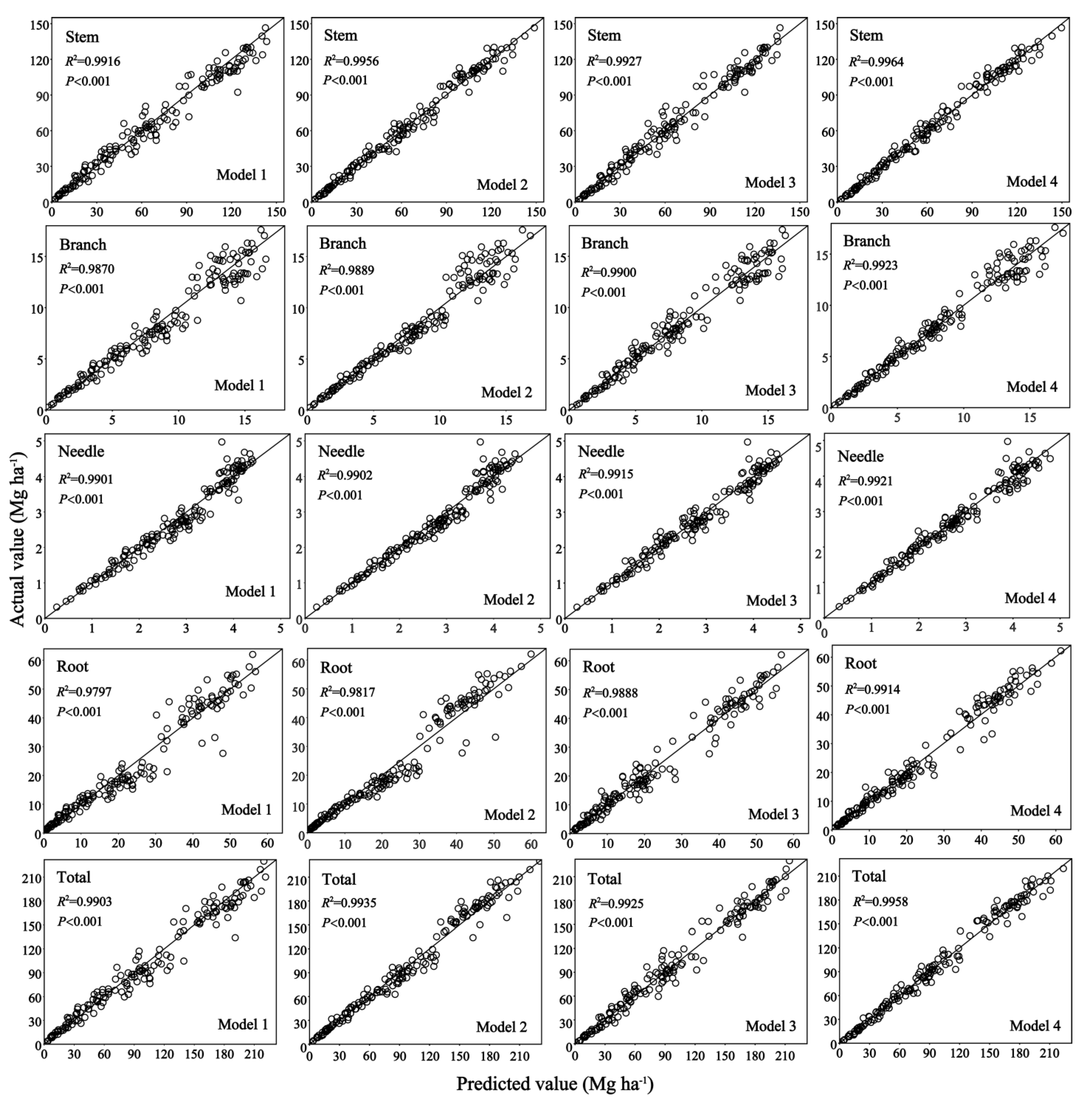
Figure 3.
Histogram of the comparison of RMSE between basic model (M-1, M-2) and proposed model (M-3, M-4) in the prediction performance for each component under four stand age groups (Young, Middle, Near-mature, Mature) for larch (Larix spp.).
Figure 3.
Histogram of the comparison of RMSE between basic model (M-1, M-2) and proposed model (M-3, M-4) in the prediction performance for each component under four stand age groups (Young, Middle, Near-mature, Mature) for larch (Larix spp.).
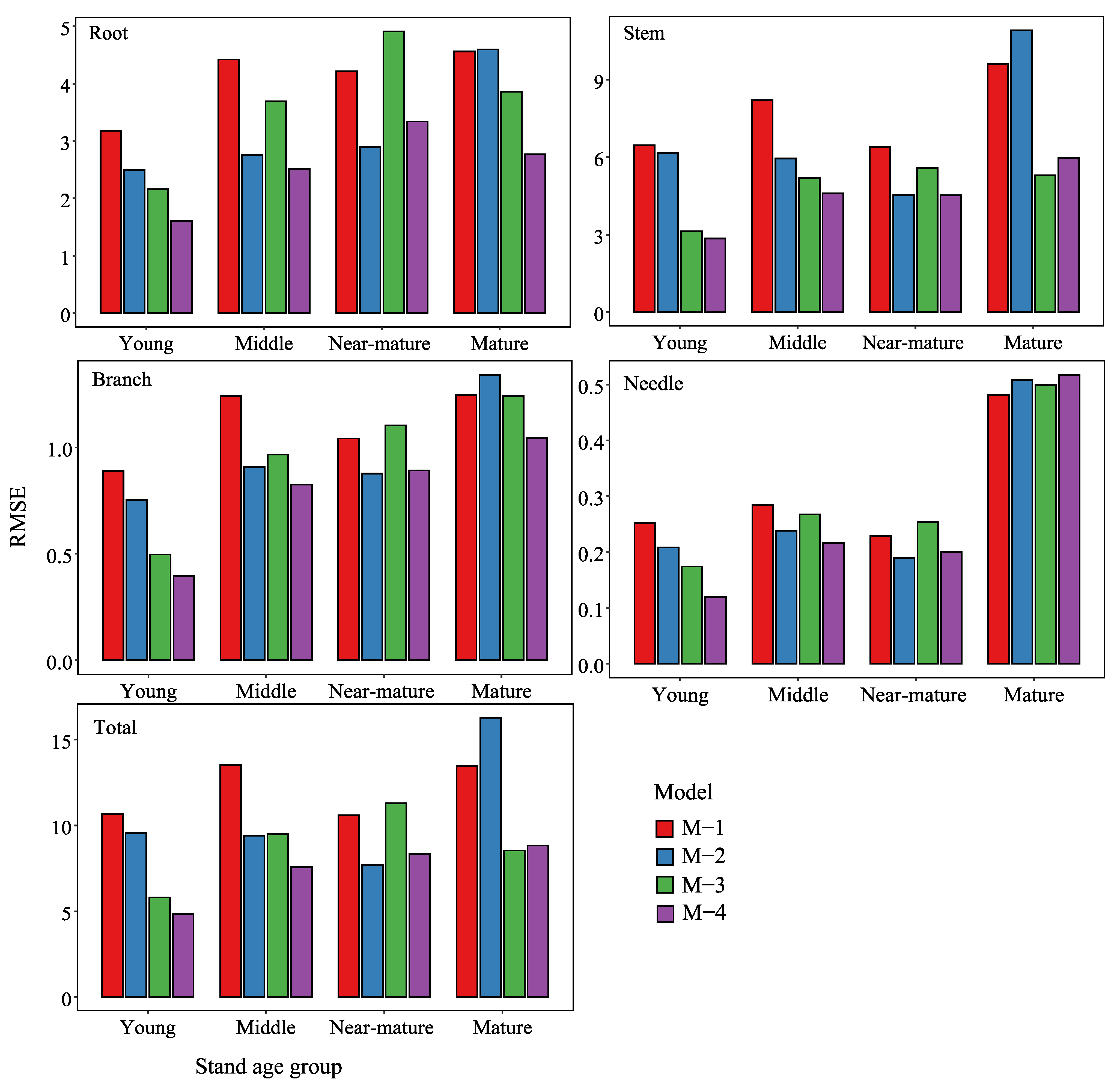
Figure 4.
Scatter plots of the actual and predicted values calculated using the comparison of the proposed stand-level biomass climate-based model of this study (M-4) and the climate-sensitive model type II (CSM-II) by He et al. [72]; the predicted value obtained by fitting our data using his model form denoted by “He et al. (2021) model fitting” (orange dots), the predicted value obtained by substituting our data into his model and using his model parameters denoted by “He et al. (2021)” (green triangles), and the predicted value obtained by the model form used in this study denoted by “This study” (blue rectangles). The red, green, and blue lines are the regression lines of the actual and predicted values.


Table 1.
Stand and climatic variables summary of larch (Larix spp.) plantations.
| Variables | Min. | Max. | Mean | SD |
|---|---|---|---|---|
| Bt (Mg·ha−1) | 1.6596 | 230.1158 | 99.7864 | 62.7069 |
| Br (Mg·ha−1) | 0.2218 | 62.0667 | 23.4326 | 17.3993 |
| Bs (Mg·ha−1) | 0.8517 | 146.5333 | 65.2729 | 39.8265 |
| Bb (Mg·ha−1) | 0.2682 | 17.6024 | 8.3023 | 4.6180 |
| Bn (Mg·ha−1) | 0.3179 | 6.5581 | 2.7786 | 1.1537 |
| BA (m2·ha−1) | 0.5500 | 34.3008 | 18.8140 | 9.4055 |
| Dg (cm) | 6.1000 | 27.3000 | 14.5093 | 3.8287 |
| Hm (m) | 4.7000 | 21.2000 | 13.7085 | 3.4106 |
| Age (year) | 5.0000 | 55.0000 | 30.4188 | 10.0592 |
| N (trees·ha−1) | 80.0000 | 3140 | 1170.6480 | 571.0343 |
| MAT (℃) | −1.1958 | 4.2875 | 2.0952 | 1.1898 |
| AP (mm) | 408.0000 | 629.0000 | 579.4375 | 38.0306 |
Abbreviations: Bt, Br, Bs, Bb, and Bn represent stand component biomass of total, root, stem, branch, and needle (Mg·ha−1), respectively. The BA, Dg, Hm, Age, and N represent the stand basal area (m2·ha−1), stand quadratic mean diameter at breast height (cm), stand mean height (m), stand age (year), and stand density (trees·ha−1), respectively. The terms MAT and AP represent annual temperature (°C) and annual precipitation (mm), respectively. The term Min. represents the minimum values, Max. represents the maximum values, and SD represents the standard deviation.
Table 2.
Parameter estimates and standard errors (SE) of stand-level biomass models.
| Model | Components | ai | bi | ci | di | fi | |||||
|---|---|---|---|---|---|---|---|---|---|---|---|
| Estimates | SE | Estimates | SE | Estimates | SE | Estimates | SE | Estimates | SE | ||
| M-1 | Total | — | — | — | — | ||||||
| Root | 0.1567 ** | 0.0136 | 1.6671 ** | 0.0259 | |||||||
| Stem | 1.0706 ** | 0.0540 | 1.3855 ** | 0.0155 | |||||||
| Branch | 0.2874 ** | 0.0124 | 1.1467 ** | 0.0134 | |||||||
| Needle | 0.3674 ** | 0.0133 | 0.7030 ** | 0.0116 | |||||||
| M-2 | Total | — | — | — | — | — | — | ||||
| Root | 0.0795 ** | 0.0109 | 1.4521 ** | 0.0206 | 0.4964 ** | 0.0515 | |||||
| Stem | 0.5799 ** | 0.0289 | 1.1646 ** | 0.0110 | 0.4743 ** | 0.0222 | |||||
| Branch | 0.1813 ** | 0.0129 | 0.9754 ** | 0.0129 | 0.3596 ** | 0.0315 | |||||
| Needle | 0.2754 ** | 0.0241 | 0.6525 ** | 0.0157 | 0.1647 ** | 0.0394 | |||||
| M-3 | Total | — | — | — | — | — | — | — | — | ||
| Root | 0.3487 ** | 0.0122 | 0.6795 ** | 0.0713 | 1.2711 ** | 0.1085 | −0.0171 ** | 0.0018 | |||
| Stem | 1.5837 ** | 0.0496 | 0.9862 ** | 0.0473 | 0.4471 ** | 0.0712 | |||||
| Branch | 0.4140 ** | 0.0126 | 0.6194 ** | 0.0532 | −0.0059 ** | 0.0016 | 0.6936 ** | 0.0807 | |||
| Needle | 0.3897 ** | 0.0134 | 0.3692 ** | 0.0472 | 0.5267 ** | 0.0696 | |||||
| M-4 | Total | — | — | — | — | — | — | — | — | — | — |
| Root | 0.1801 ** | 0.0100 | −0.0054 ** | 0.0007 | 0.5167 ** | 0.0497 | 1.2493 ** | 0.0777 | 0.4360 ** | 0.0270 | |
| Stem | 0.7178 ** | 0.0436 | 0.8753 ** | 0.0366 | 0.3854 ** | 0.0506 | 0.4649 ** | 0.0269 | |||
| Branch | 0.2367 ** | 0.0174 | −0.0042 ** | 0.0011 | 0.5230 ** | 0.0491 | 0.6501 ** | 0.0714 | 0.3501 ** | 0.0344 | |
| Needle | 0.2823 ** | 0.0153 | −0.0049 ** | 0.0013 | 0.3153 ** | 0.0450 | 0.4960 ** | 0.0673 | 0.2172 ** | 0.0294 | |
Notes: M-1 and M-2 for stand-level biomass basic model types 1 and 2, M-3 and M-4 for stand-level biomass climate-based model types 3 and 4, respectively. SE is the standard error, and ai, bi, ci, di, and fi are the model parameters. The asterisks (**) represent the coefficient estimates at the significance p < 0.001.
Table 3.
The goodness-of-fit statistics and weight functions of the stand-level biomass models.
| Model | Components | R2 | RMSE | Weight Functions |
|---|---|---|---|---|
| M-1 | Total | 0.9636 | 11.9599 | BA1.3139 |
| Root | 0.9441 | 4.1141 | BA1.0188 | |
| Stem | 0.9644 | 7.5111 | BA1.3991 | |
| Branch | 0.9422 | 1.1102 | BA1.5266 | |
| Needle | 0.9322 | 0.3004 | BA0.5263 | |
| M-2 | Total | 0.9779 | 9.3159 | BA1.7658Hm−0.8141 |
| Root | 0.9503 | 3.8780 | BA1.0090 | |
| Stem | 0.9844 | 4.9754 | BA1.6903 | |
| Branch | 0.9542 | 0.9879 | BA1.4848 | |
| Needle | 0.9349 | 0.2943 | BA0.2356 | |
| M-3 | Total | 0.9743 | 10.0582 | BA1.2663 |
| Root | 0.9697 | 3.0309 | BA2.0758 | |
| Stem | 0.9738 | 6.4489 | BA1.6641 | |
| Branch | 0.9592 | 0.9330 | BA1.5172 | |
| Needle | 0.9438 | 0.2735 | BA0.9103 | |
| M-4 | Total | 0.9856 | 7.5167 | BA1.6287 |
| Root | 0.9763 | 2.6811 | BA2.4416 | |
| Stem | 0.9874 | 4.4725 | BA1.4808 | |
| Branch | 0.9689 | 0.8149 | BA1.4973 | |
| Needle | 0.9479 | 0.2633 | BA0.6226Hm1.8235 |
Table 4.
The validation result of the larch (Larix spp.) plantation’s stand-level biomass models.
| Model | Components | RMSE | RMSPE | MAE | MAPE | MPE |
|---|---|---|---|---|---|---|
| M-1 | Total | 12.1564 | 0.1499 | 8.6032 | 11.2165 | 8.6216 |
| Root | 4.1812 | 0.2305 | 2.8486 | 17.1401 | 12.1564 | |
| Stem | 7.5914 | 0.1428 | 5.5935 | 10.8353 | 8.5695 | |
| Branch | 1.1228 | 0.1422 | 0.8521 | 11.4392 | 10.2638 | |
| Needle | 0.3006 | 0.0929 | 0.1866 | 7.0029 | 6.7151 | |
| M-2 | Total | 9.4978 | 0.1032 | 6.7471 | 7.9600 | 6.7615 |
| Root | 3.9706 | 0.1912 | 2.7974 | 14.8200 | 11.9382 | |
| Stem | 5.0620 | 0.0922 | 3.6382 | 6.8980 | 5.5738 | |
| Branch | 1.0029 | 0.1046 | 0.7004 | 8.3834 | 8.4356 | |
| Needle | 0.2981 | 0.0831 | 0.1761 | 6.2375 | 6.3369 | |
| M-3 | Total | 10.2127 | 0.1331 | 7.2904 | 9.7924 | 7.3060 |
| Root | 3.0923 | 0.1702 | 2.2026 | 12.5073 | 9.3996 | |
| Stem | 6.5462 | 0.1344 | 4.6312 | 9.7138 | 7.0951 | |
| Branch | 0.9499 | 0.1211 | 0.7232 | 9.6681 | 8.7108 | |
| Needle | 0.2781 | 0.0841 | 0.1652 | 6.1731 | 5.9467 | |
| M-4 | Total | 7.6593 | 0.0958 | 5.5504 | 7.0569 | 5.5623 |
| Root | 2.7315 | 0.1356 | 1.9177 | 10.0865 | 8.1837 | |
| Stem | 4.5711 | 0.0961 | 3.2952 | 6.7650 | 5.0483 | |
| Branch | 0.8335 | 0.0953 | 0.5991 | 7.4924 | 7.2163 | |
| Needle | 0.2690 | 0.0715 | 0.1498 | 5.1831 | 5.3904 |
Abbreviations: RMSE is the root mean square error (%), RMSPE is the root mean square prediction error (%), MAE is the mean absolute error (%), MAPE is the root mean square prediction error (%), and MPE is the mean prediction error (%).
Disclaimer/Publisher’s Note: The statements, opinions and data contained in all publications are solely those of the individual author(s) and contributor(s) and not of MDPI and/or the editor(s). MDPI and/or the editor(s) disclaim responsibility for any injury to people or property resulting from any ideas, methods, instructions or products referred to in the content. |
© 2023 by the authors. Licensee MDPI, Basel, Switzerland. This article is an open access article distributed under the terms and conditions of the Creative Commons Attribution (CC BY) license (https://creativecommons.org/licenses/by/4.0/).
Share and Cite
MDPI and ACS Style
Mahardika, S.B.; Xin, S.; Wang, W.; Jiang, L. Effects of Climate on Stand-Level Biomass for Larch Plantations in Heilongjiang Province, Northeast China. Forests 2023, 14, 820. https://doi.org/10.3390/f14040820
AMA Style
Mahardika SB, Xin S, Wang W, Jiang L. Effects of Climate on Stand-Level Biomass for Larch Plantations in Heilongjiang Province, Northeast China. Forests. 2023; 14(4):820. https://doi.org/10.3390/f14040820
Chicago/Turabian StyleMahardika, Surya Bagus, Shidong Xin, Weifang Wang, and Lichun Jiang. 2023. "Effects of Climate on Stand-Level Biomass for Larch Plantations in Heilongjiang Province, Northeast China" Forests 14, no. 4: 820. https://doi.org/10.3390/f14040820
Note that from the first issue of 2016, this journal uses article numbers instead of page numbers. See further details here.