Examining the Spatial Mode, Supply–Demand Relationship, and Driving Mechanism of Urban Park Green Space: A Case Study from China

Abstract

Park green space is a big part of public infrastructure in cities, and how to evaluate and optimize the mismatch of urban park green space (UPGS) has become the focus of current research in academia and industry. Taking China’s 286 cities as an example, this paper used the spatial cluster and Boston Consulting Group Matrix to analyze the aggregation laws and changing modes of UPGS from 2010 to 2020, introduced the spatial mismatch model to analyze the matching of its supply and demand with GDP and population, and adopted the Geodetector to analyze the influencing factors. The findings: (1) The evolution of UPGS in China had long been characterized by a “pyramidal” pattern, i.e., limited green cities > developing green cities > steady green cities > booming green cities, exhibiting the spatial characteristics of gradient differences between the coasts and inland areas, and the aggregation of blocks in some areas. (2) The supply and demand mismatches of the UPGS were relatively stable, with negative matching being the main supply mismatch type, and positive matching being the main demand mismatch type. The contribution of supply and demand mismatches similarly showed a spatial pattern of a gradual decrease from the coast to inland and the aggregation of blocks in some areas. (3) Five types of factors played different driving roles on UPGS, with social development remaining a weak factor, and the strong factor switching from urban infrastructure to construction land scale. The interaction detection was dominated by a bilinear enhancement, with super-interaction factors changing from an output value of the tertiary industry and population urbanization rate to education expenditure in local general public budgets. (4) Based on the mismatch between the supply and demand for UPGS in China, 286 cities were classified into four types, namely a smart shrinking zone, smart growing zone, status quo zone, and overlay policy zone, and differentiated development proposals for the corresponding zoning were put forward. This paper constructed an application framework of “evolution pattern + supply demand match + driving factors + policy zoning” for UPGS at a large scale, which will effectively enhance the effective allocation of its resources across the country.

1. Introduction

1.1. Background

As a significant component of public infrastructure, urban park green space (UPGS) plays ecological service functions such as purifying the environment, regulating the microclimate, conserving water, and maintaining biodiversity, in addition to the social service functions [1,2] of disaster prevention and mitigation, education and popularization of science and technology, leisure and recreation, and it is even closely related to the wellbeing of the residents and their quality of life [3]. It is also for this reason that UPGS has always been the focus of urban geography and planning research. UPGS is characterized by clear spatial attributes, and its spatial configuration potentially affects the effectiveness and equality of ecological and social benefits, which, in turn, jeopardizes the sustainable development of the city. Therefore, international organizations as well as some countries have put forward requirements on UPGS per capita, for example, the per capita area for UPGS is 30 m² according to the United Nations, 26 m² in the European Union, 18 m² in the United States, and 8~14.6 m² in China [4,5]. However, the inherent “human–land conflict” in urban areas and the poor management or disorderly construction of some cities have led to the frequent mismatch between the construction of urban parks and the development of the city, i.e., the mismatch of UPGS resources [6,7]. How to evaluate and optimize the mismatch of UPGS has been a crucial problem to be solved urgently for the academia and the industry. The mismatch may be found at macro, meso, and micro scales, and the supply–demand relationship and evolution mechanism at different scales are obviously different [8,9], making it necessary to also conduct differential research on them.

With the rapid advance of urbanization, UPGS construction in China has also made great progress since the reform and opening up, with the UPGS area growing from 21,600 hectares in 1981 to 797,900 hectares in 2020, an increase of 37 times, and the per capita UPGS area correspondingly growing from 1.5 m² to 14.78 m², an increase of 10 times [8]. Nevertheless, the current per capita UPGS area in China is still low by international standards and those of developed countries. In addition, given the differences in the development foundation and development process of different regions in China, UPGS is also facing a very prominent problem of uneven distribution [9]. Insufficient quantity and uneven distribution have seriously impeded the equality and fairness of public services in UPGS for urban residents, and how to make up for the two has also become the focus of China’s promotion of the equalization of basic public services during the “14th Five-Year Plan” period. Therefore, this paper’s exploration of the evolutionary patterns of UPGS and the mismatch between supply and demand based on the case study of China is quite typical.

1.2. Literature Review

There are currently few studies on UPGS oriented to “supply–demand match” in academia, but the integration of social and economic factors into UPGS research has long been a common paradigm, and relevant results are mainly reflected in the discussion on the matching and accessibility between UPGS and the population, economy, and land use at regional and urban scales.

At the regional scale, Song et al. portrayed the supply and demand relationship of UPGS in 284 cities in China using the per capita UPGS area, and looked into the influencing factors in the three dimensions of urban background conditions, socio-economic factors, and public policy environment [9]. Wu et al. calculated the equality of UPGS use in 341 cities in China by counting the UPGS area in the buffer zone of the population grid, and pointed out that GDP per capita, population density, and built-up land area had an obvious effect on it [10]. Huang et al. calculated the accessibility of green space to population in 366 cities in China by two-step move search, and explored the impact of urban expansion on the change of green space accessibility [11]. Wu et al. assessed the equity of green space use among different socioeconomic groups in urban areas of China by calculating three indicators, namely, vegetation coverage, park area coverage, and proximity to parks, based on large-scale survey data [12]. Li et al. explored the equity of green space in 58 cities in China using three indicators: green space per capita, green coverage rate, and green space within 1500 m of the community, and pointed out that climate, urban topography, proportion of secondary industry, and title incentive factors had an obvious effect on it [13]. Long et al. calculated the green space accessibility of 4353 cities worldwide using the number of people within the green space buffer [14]. Kabisch et al. calculated the availability of green space in 299 EU cities using the number of people in the green space buffer zone [15]. Wolff et al. calculated inequalities in green space accessibility in 899 European cities using the number of people in the green space buffer zone [16]. Wüstemann et al. calculated inequalities in access to green space in 53 German cities using the area of green space within the buffer zone of the population grid [17]. Huang et al. evaluated changes in the availability of green space in 28 megacities around the world using two indicators: the percentage of green space area and the number of people in the green space buffer zone [18]. Richards et al. used green space coverage and green space per capita to reflect the availability of green space in Southeast Asian cities [19].

At the urban scale, Gupta et al. evaluated the availability of green space in areas of Delhi (India) at different stages of development through GIS network analysis [20]. Huerta et al. evaluated differences in neighborhood green space accessibility across economic levels in Mexico City (Mexico) through GIS network analysis [21]. Sikorska et al. validated the role of informal green spaces in increasing the availability of green spaces for the elderly and children in Warsaw and Łódź (Poland) by the buffer approach [22]. Xu et al. compared the availability of green space in Munich (Germany) under different development scenarios using two indicators: green space area per capita and population with green space [23], and further calculated the changes in green space equity in Munich under different development scenarios using the area of green space within the population grid buffer zone [24]. Fan et al. explored the spatio-temporal evolution of the green space accessibility of residential parks around Shanghai (China) in the context of rapid urbanization by constructing a green accessibility index [25]. Cetin compared the differences in the availability of green space in Kutahya (Turkey) in terms of the area of parkland per capita [26]. Ye et al. calculated the green space accessibility differences among different populations in Macau (China) by a two-step move search [27]. Chen et al. analyzed the differences in the accessibility of green spaces in Hannover (Germany) among different age groups, especially the elderly, by a two-step mobile search [28]. Liu et al. analyzed differences in green space accessibility across ethnicity and income groups in Chicago (America) by a two-step move search [29]. Zhang et al. improved the two-step move search using cell phone signaling big data and the PageRank algorithm to study the accessibility of UPGS for different populations in Shenzhen (China) [30]. Li et al. improved the two-step move search to analyze the accessibility of parks in different neighborhoods of Xuzhou (China) by taking different travel modes and park quality into account [31]. Ma improved the accessibility model with spatial syntax and demographic data and calculated the green space accessibility in Jinan (China) [32]. Ghasemi et al. improved the accessibility calculation method and analyzed the equity of green space in Tehran (Iran) using a combined compromise solution [33]. Pinto et al. compared the difference in the accessibility of green spaces in Vilnius (Lithuania) and Coimbra (Portugal) by calculating the coverage of different travel modes [34]. Buckland et al. compared the differences in green space accessibility of five medium-sized European cities using GIS network analysis [35]. Schindler et al. reflected on the inadequacy of conventional accessibility calculation methods by modeling the distances between residents and frequented UPGS in three European cities based on questionnaire data [36]. Xing et al. represented supply and demand using the UPGS and the population size, calculated the change to their relationship in Wuhan (China) by a two-step move search [7]. Yang et al. explored the supply–demand relationship of green space in Beijing against flooding disasters using green space and population size to represent supply and demand through a two-step move search [37].

Although research on the “supply–demand match” of UPGS (green land) has yielded extensive research findings, two shortcomings have been identified. First, methodologically, most of the existing studies, whether at the regional or urban scale, have revealed the green space supply and demand by calculating its accessibility to the population and communities. However, this method is characterized by great calculation difficulty and restricted application scenarios, and the variables representing their relationship as well as the calculation methods still need to be further expanded. Second, as for the framework, the available studies focus on the evaluation of spatial distribution differences or the inequalities of UPGS, but there are few efforts on policy zoning and planning regulation, which goes against guiding the effective distribution of UPGS resources among regions. How to effectively link theoretical analysis and practical applications still needs to be further explored.

1.3. Aim and Question

Therefore, taking China as an example, this paper focuses on analyzing the evolution and mismatch between supply and demand from a macro perspective, and attempts to build an integrated framework of “evolution mode + supply–demand matching + driving factors + policy zoning”, helping to deeply understand the “human–land relationship” of UPGS on a large scale and guiding the effective construction of UPGS. By matching UPGS with the economy and population, this paper shows the economic carrying capacity with the former, which is used to represent the financial supply capacity of green space, and shows the population size with the latter, which is used to characterize the intensity of residents’ consumption demand.

This paper is mainly to address the following issues: (1) What are the spatial patterns and changing modes of UPGS in China? (2) What are the supply–demand mismatch types of UPGS with GDP and population in China? (3) What are the direct action factors and interaction factors of UPGS in China? (4) How to conduct policy zoning and put forward optimization proposals based on the mismatch relation of UPGS?

2. Materials and Methods

2.1. Study Area: China

This paper selected 286 cities in mainland China as the study area, located in 30 provinces (autonomous regions and municipalities directly under the central government), with exclusion of Tibet due to the shortage of data, as well as Hong Kong, Macao, and Taiwan due to inconsistencies in their statistical systems (Figure 1). This paper sets 2010–2020 as the study period considering two reasons. First, the report of the 18th National Congress of China in 2012 set up the general outline of “ecological civilization construction”, and subsequently the relevant plans were developed across China based on it to promote urban greening construction. Second, the span of the period coincides with the two policy periods of “Twelfth Five-Year Plan” and “Thirteenth Five-Year Plan”, which ensures the reliability of the conclusions to a greater extent with the development policies in the corresponding period staying relatively stable.

2.2. Index Selection and Data Acquisition

This paper studies the UPGS, which is the city’s “regular green space”, led by the government in integrated planning, investment, construction, and maintenance management. It is directly affected by local government finances and in turn directly provides recreational space for residents. In fact, only by matching with economic development and population distribution can UPGS meet residents’ consumption demand without bringing too much financial burden [38,39,40]. Therefore, UPGS area is taken as the basic element, urban GDP is taken as the supply element, and urban population is taken as the demand element (

Table 1. Dependent, independent, and supply–demand variable description.

Variables	Code	Indicators	Implication
Dependent variable	$Y_1$	Area of urban UPGS in 2010 (ha)	Area scale
	$Y_2$	Area of urban UPGS in 2020 (ha)
Independent variable	$X_1$	Output value of secondary industry (100 million CNY)	Industry development
	$X_2$	Output value of the tertiary industry (100 million CNY)
	$X_3$	Population urbanization rate (%)	Social development
	$X_4$	Average wage of employed staff and workers (CNY)
	$X_5$	Area of land used for urban construction (square kilometer)	Construction land scale
	$X_6$	Area of land used for living (square kilometer)
	$X_7$	Local general public budget expenditure (10,000 CNY)	Public budget expenditure
	$X_8$	Education expenditure in local general public budget (10,000 CNY)
	$X_9$	Area of city paved roads (10,000 square meter)	Urban infrastructure
	$X_{10}$	Number of buses and trolley buses under operation (vehicle)
Supply and demand variable	$Z_1$	Supply: GDP (100 million CNY)	Matching elements
	$Z_2$	Demand: Population (10,000 person)

).

The key condition that affects the match between UPGS supply and demand is the UPGS in the constructed framework, and it is also the UPGS that lies in the core of regulating the relationship between supply and demand. Therefore, according to related research [9,10,12,13,41,42,43], this paper explores the factors affecting the spatial differentiation of UPGS in five dimensions: industrial development, social development, scale of construction land, and public budget expenditure. The details are analyzed below:

(1)

Industrial development is the basic economic driving force for the construction of UPGS, while secondary and tertiary industries are the economic pillars of the city. This paper uses output value of secondary industry ($X_1$) and output value of tertiary industry ($X_2$) to represent the industrial development;

(2)

Social development presents the demand of urban residents for the construction of UPGS, while urbanization is a reflection of the comprehensive development of society [44,45], and the wages of employees are a reflection of the level of income of residents, so this paper chooses population urbanization rate ($X_3$) and average wage of employed staff and workers ($X_4$) to represent social development;

(3)

Since construction land both provides sites for UPGS construction and has supporting requirements for UPGS, and thus stimulates UPGS construction [46,47], this paper chooses area of land used for urban construction ($X_4$) and area of land used for living ($X_5$) to represent the scale of construction land;

(4)

Fiscal expenditure reflects the level of administrative support for the construction of UPGS, and also stimulates its consumption demand by supporting other social undertakings (such as education and culture) [48,49], so this paper selects local general public budget expenditure ($X_7$) and education expenditure in local general public budgets ($X_8$) to represent public financial expenditure;

(5)

Infrastructure provides a hardware environment for UPGS construction by improving accessibility and increasing water supply and power supply [9,50], so this paper chooses area of city paved roads ($X_9$) and number of buses and trolley buses under operation ($X_{10}$) to represent urban infrastructure.

The data in this study is based on the China Urban Statistical Yearbook and the China Urban Construction Statistical Yearbook. To ensure that the calculation results are more accurate, the statistical scope of all data is uniformly limited to municipal districts. Limited by the data, $X_4$ stands for the average wage across the city and, given that most jobs are concentrated in the municipal districts of cities in China, $X_4$ represents the average wage in the municipal districts.

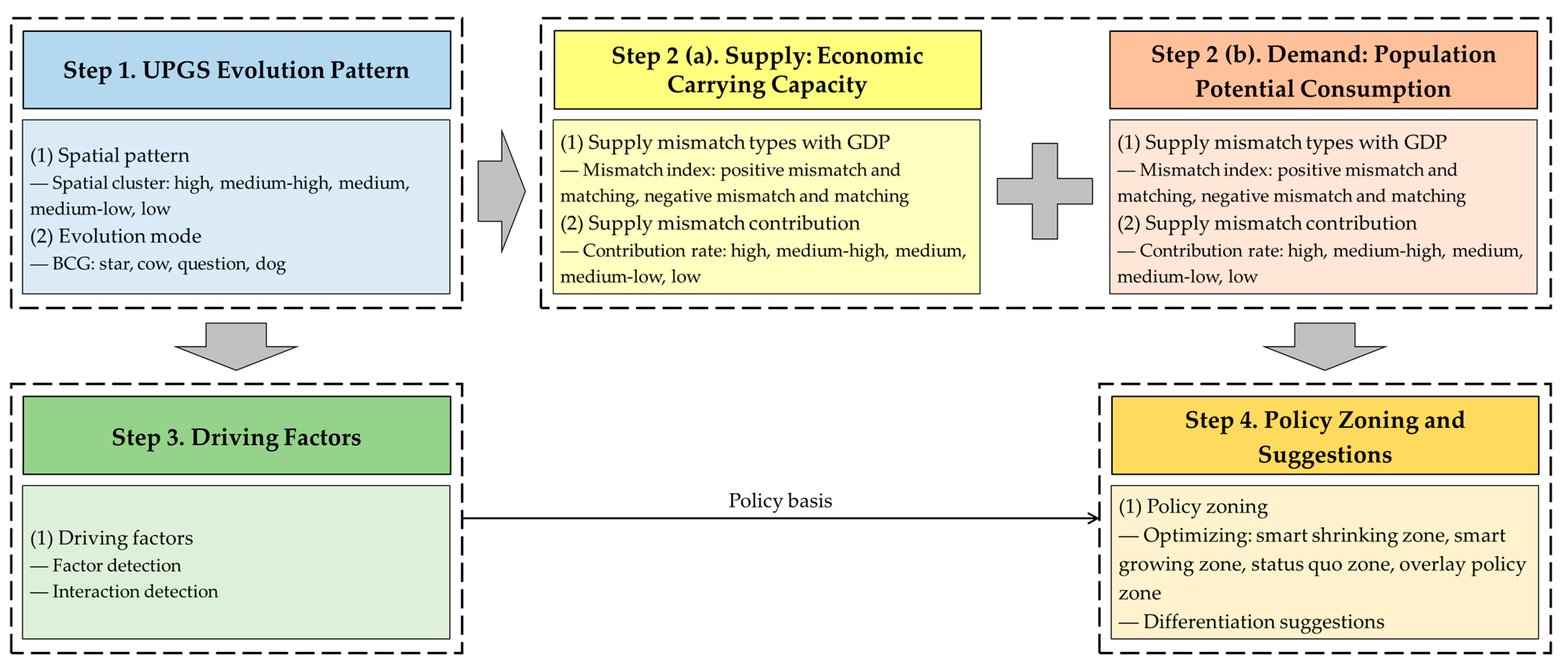
2.3. Research Frame

The study is conducted by 4 steps (Figure 2). Step 1 is to explore the spatial distribution differences of UPGS in 286 cities in China through spatial clustering, analyzing its evolution pattern using the BCG matrix. Step 2 is to investigate the supply–demand mismatch, analyzing the mismatch type using the spatial mismatch index, analyzing the mismatch contribution using the contribution model. Step 3 is to study driving factors, analyzing the influencing factors that lead to differences in the spatial distribution of UPGS using Geodetector, including the direct action and interaction of factors. Step 4 is about policy zoning and suggestions, deriving the policy zoning of UPGS development using the supply–demand matching model, and putting forward differentiated development suggestions.

2.4. Research Methods

2.4.1. Boston Consulting Group Matrix

Boston Matrix is mainly applied in the fields of business management and economics, which divides products or markets into star, cow, problem, and dog types according to the matching of both factors “market share” and “sales growth” [51,52]. It is borrowed to analyze the changing mode of UPGS. The equation is shown below:

$$RS=\frac{y_i}{y_{max}}, GR=\sqrt[a]{\raisebox{1ex}{$y_i$}\!\left/ \!\raisebox{-1ex}{$y_i^{\prime }$}\right.}-1$$

(1)

where, RS is the relative proportion of UPGS in city i, GR is the growth rate of UPGS in city i, $y_i$ is UPGS in city i, $y_{max}$ is the maximum UPGS, $y_i^{\prime }$ is UPGS in city i in the base period, and a is the year span of the study interval. To eliminate human interference, this paper chooses the average value of relative share and growth rate as the threshold, and divides the changing modes of UPGS into star, cow, question, and dog types. Meanwhile, to fit the context better, this paper also renames the cities corresponding to these four patterns as booming, steady, developing, and limited green cities. Booming green cities have large UPGS areas and high growth rates, steady green cities have large UPGS areas but low growth rates, developing green cities have small UPGS areas but high growth rates, and limited green cities have small UPGS areas and low growth rates.

2.4.2. Spatial Mismatch Model

The spatial mismatch hypothesis, raised by Kain in the 1960s, was initially introduced to explore the spatial connection between residence and employment in the context of residential suburbanization [53], and was later extended to study the incomplete matching in spatial distribution of interrelated elements [54,55]. This paper employs the spatial mismatch index to portray the spatial matching of UPGS with GDP and population, which is based on Liu and Theys et al. for the calculation model [56,57].

(1)

Spatial mismatch index is used to show the mismatch index and type of UPGS. The equation is as follows:

$${SMI}_i=\frac{\left(\frac{x_i}{x}\times y-y_i\right)}{2y}\times 100\%$$

(2)

where, ${SMI}_i$ is the spatial mismatch index of city i, $x_i$ and $x$ represent the population size and total GDP of city i and the sum of population and GDP of all cities, respectively, and $y_i$ and $y$ represent the UPGS area of city i and the sum of UPGS area of all cities, respectively. When ${SMI}_i$ is to 0, it means that the UPGS resource of the city just matches with the population demand and economic carrying capacity; when ${SMI}_i$ is less than 0, it means that the UPGS resource of the city is insufficient and cannot meet the actual demand of residents or is lower than the economic carrying capacity; ${SMI}_i$ more than 0 means excessive UPGS resource supply, going beyond the actual demand of residents or the economic carrying capacity. A larger absolute value of ${SMI}_i$ indicates a higher degree of UPGS mismatch. To facilitate the analysis, the spatial mismatches are further classified into positive mismatch, positive matching, negative matching, and negative mismatch using positive and negative ${SMI}_i$, and 0 as thresholds (

Table 2. Spatial mismatch types, mathematical relationship, and practical meaning.

Type	Relationship	Meaning
Positive mismatch	$SMI>\overline{SMI}, SMI>0$	UPGS resources are greater than the demand of residents or economic carrying capacity, with a serious oversupply and a high degree of mismatch.
Positive matching	$0<SMI<\overline{SMI}, SMI>0$	UPGS resources are greater than the demand of residents or economic carrying capacity, with a slight oversupply and a low degree of mismatch.
Negative matching	$0>SMI>\overline{SMI}, SMI<0$	UPGS resources are less than the demand of residents or greater than economic carrying capacity, with a slight shortage of supply and a low degree of mismatch.
Negative mismatch	$SMI<\overline{SMI}, SMI<0$	UPGS resources are less than the demand of residents or greater than economic carrying capacity, with a serious shortage of supply and a high degree of mismatch.

).

(2)

Contribution rate index is used to show the impact of a city on the UPGS mismatch in the study area. The equation is as follows:

$$SMI=\frac{{\sum }_{i=1}^n\left|\frac{x_i}{x}\times y-y_i\right|}{2y}, C_i=\frac{\left|{SMI}_i\right|}{SMI}\times 100\%$$

(3)

where, $SMI$ is the sum of the absolute values of the spatial match indices of all cities, $C_i$ is the contribution of city i to the spatial match of all cities, and the other variables have the same meanings as above. A larger value of $C_i$ indicates that the city contributes more to the mismatch in all cities.

2.4.3. Geodetector

Geodetector is a spatial analysis model designed for detecting the spatial heterogeneity of geographic elements and their driving factors. Compared with the traditional regression methods, Geodetector shows clear advantages, such as being free from factor collinearity interference and increasing the analysis of interaction between factors. It has been used in extensive research fields, such as natural and humanities and social sciences [58,59,60,61]. Geodetector contains many modules, and this paper employs factor detection and interaction detection to analyze the influencing factors of the UPGS differentiation.

(1)

Factor detection is to detect the explanation index of spatial differentiation of a factor to the dependent variable, calculated as follows:

$$q=1-\frac{1}{N{\sigma }^2}\sum _{h=1}^L{N}_h{\sigma }_h^2$$

(4)

where, q measures the driving force on the UPGS differentiation, N is 286, the total number of city samples, with h = 1, 2, 3, … L, where L is the number of partitions or strata, ${\sigma }^2$ is the total dispersion variance of the UPGS area, and ${\sigma }_h^2$ is the dispersion variance of the UPGS area in the h-th partition or stratum. The value of q is in the range of [0, 1], with a larger value indicating a stronger explanatory power of the independent variable X for Y.

(2)

Interaction detection is to identify whether the explanatory power for the dependent variable is enhanced or diminished when 2 independent variables act together. A total of five interaction results were identified using Geodetector, i.e., nonlinearly weaken, unilinearly weaken, bilinearly strengthened, nonlinearly strengthened, and mutually independent (

Table 3. Interaction effect relationship, as cited in reference [58].

Graphical Representation	Description	Interaction
	q($X_i$∩$X_j$) < min(q($X_i$), q($X_j$))	Weaken, nonlinear
	min(q($X_i$), q($X_j$)) < q($X_i$∩$X_j$) < max(q($X_i$), q($X_j$))	Weaken, uni-
	q($X_i$∩$X_j$) > max(q($X_i$), q($X_j$))	Enhance, bi-
	q($X_i$∩$X_j$) > q($X_i$) + q($X_j$)	Enhance, nonlinear
	q($X_i$∩$X_j$) = q($X_i$) + q($X_j$)	Independent
Legend:    min(q($X_i$), q($X_j)$)    max(q($X_i$),    q($X_j$)) q($X_i$) + q($X_j$)     q($X_i$∩$X_j$)

).

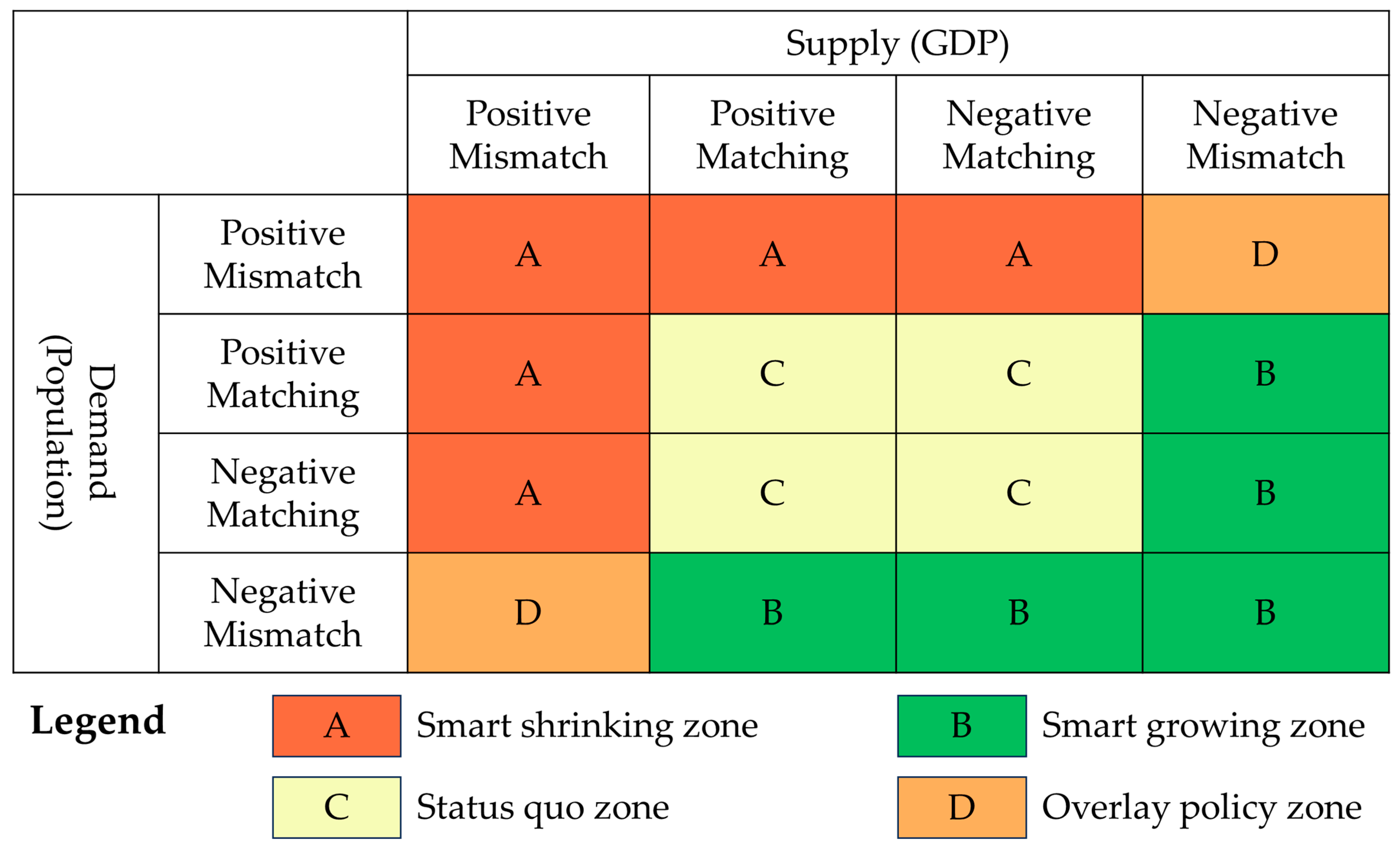
2.4.4. Policy Zoning Framework

According to the supply–demand mismatch types, this paper proposes a new policy zoning framework for UGPS, in which the UPGS can be divided into four policy zones, namely a smart shrinking zone, smart growing zone, status quo zone, and overlay policy zone (Figure 3). The four policy zones have different development focuses:

(1)

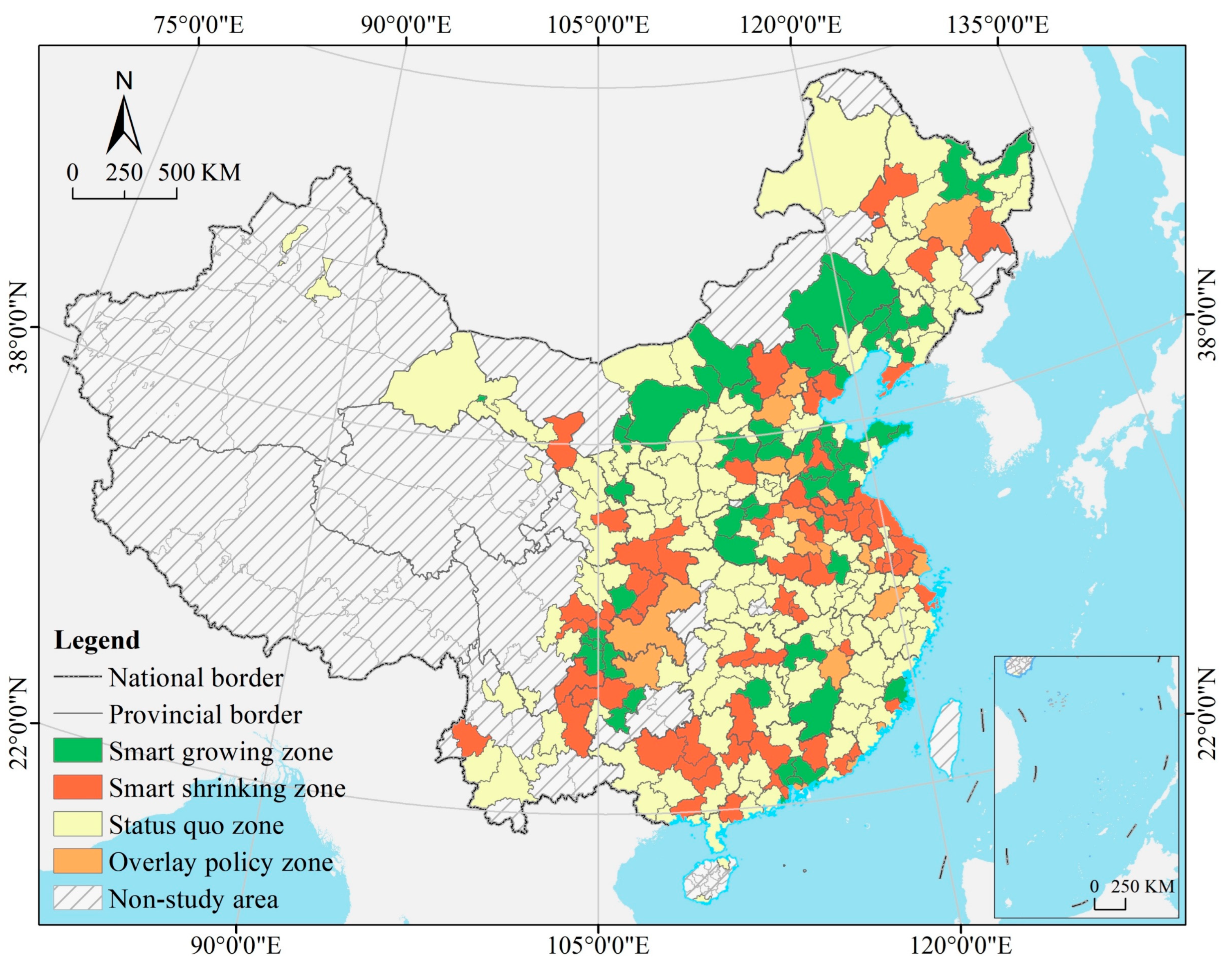
In smart shrinking zones, UPGS is in oversupply, beyond actual demand or (and) above the economic carrying capacity, a smart shrinking strategy for UPGS should be implemented;

(2)

In smart growing zones, UPGS is in short supply, less than actual demand, or (and) below economic carrying capacity, a smart growing strategy for UPGS should be implemented;

(3)

In status quo zones, the supply and demand of UPGS are in a dynamic balance and stay in an optimal state, the status quo development strategy should be maintained to provide reference for the policy design of other zonings;

(4)

In overlay policy zones, UPGS, due to the double mismatch of supply and demand, is lower than the actual demand but greater than the economic carrying capacity, or greater than the actual demand but lower than the economic carrying capacity. For the former case, additional investment should be made in the form of a transfer payment to increase UPGS, and for the latter case, the trans-regional transfer payment for support should be increased to control the increment of UPGS.

3. Results

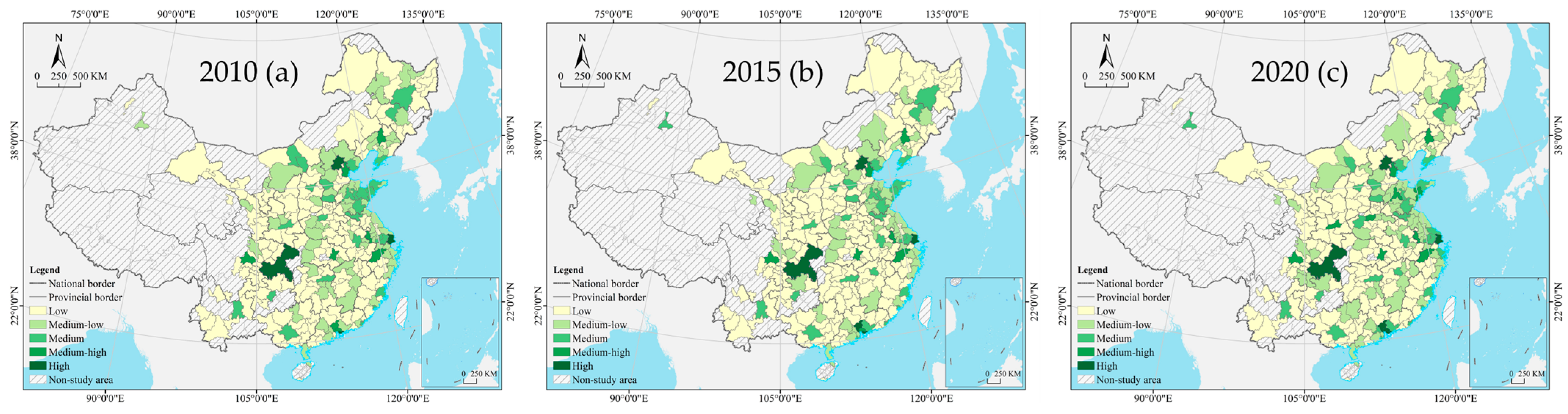
3.1. Spatial Evolution Pattern on UPGS

3.1.1. Spatial Pattern and Changing Mode on UPGS

The UPGS area of 286 cities was categorized into five types of high, medium-high, medium, medium-low, and low cities by natural breakpoint (Figure 4). It is clear that the UPGS in China has a relatively stable spatial pattern, generally showing the spatial characteristics of a coastal–inland gradient difference and block-like aggregation in some areas. In 2010, high, medium-high, medium, medium-low, and low cities accounted for 1.40%, 2.80%, 9.79%, 26.22%, and 59.79%, respectively, while accounting for 1.75%, 2.45%, 10.49%, 19.58%, 65.73% in 2015, and 2.10%, 3.50%, 10.49%, 22.73%, 61.19% in 2020. There was a small number of high and medium-high cities, increasing from only 12 in 2012 and 2015 to 15 in 2020. Medium cities are scattered in distribution, mostly including provincial capitals and key cities, with agglomeration appearing in Shandong in 2012, but weakened in 2015 and 2020. Medium-low cities were distributed in blocks, mainly in central and east China, with a small number in the west and northeast, gradually growing into two aggregations in the Shandong Peninsula and the Yangtze River Delta, and appearing in blocks in Inner Mongolia, Liaoning, Hebei, Sichuan, Guangdong, Guangxi, Hunan, Jiangxi, and Henan. Low cities contracted somewhat but remained scattered as a mainstay across most of the country.

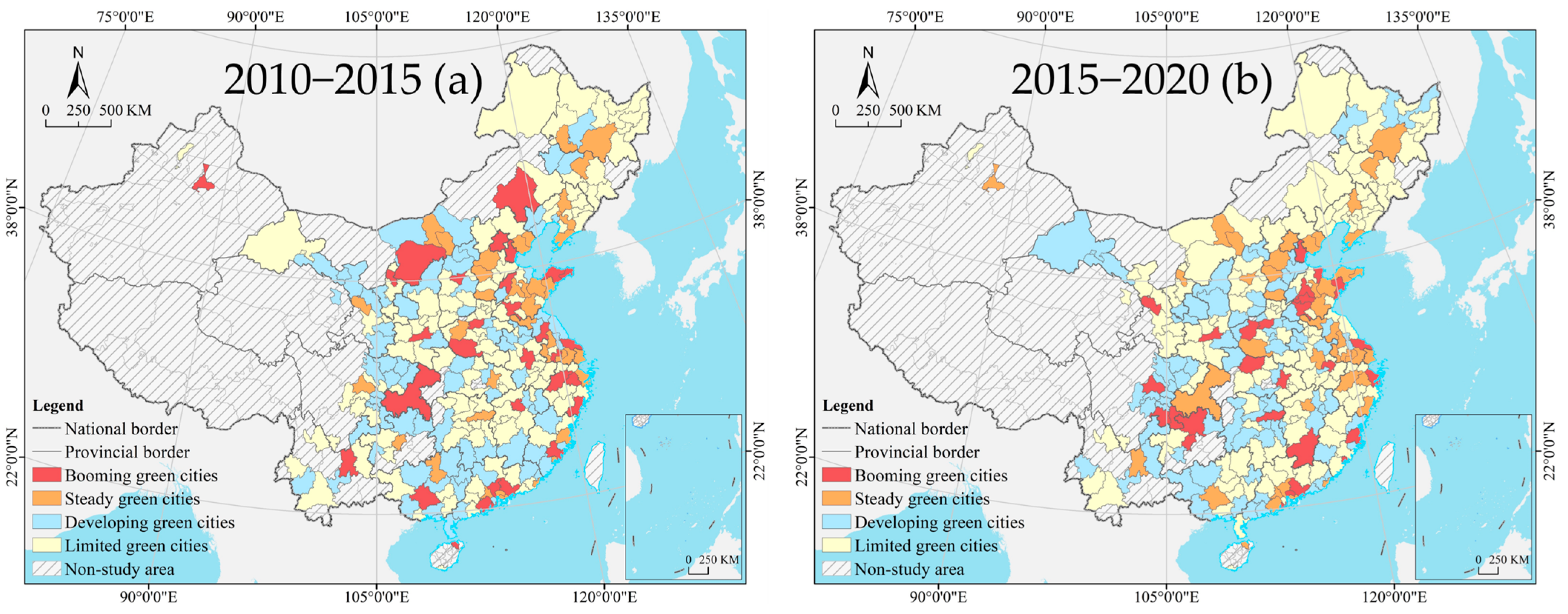
3.1.2. Spatial Changing Mode on UPGS

The study period was equally divided into 2010–2015 and 2015–2020 to explore the change patterns of UPGS in each time frame (Figure 5). It can be seen that the cities with four types of evolution patterns of UPGS in China showed a “pyramid” structure with a relatively stable number, and the cities with better evolution were found in the central and eastern regions of the country, as well as in the major provincial capitals and key cities. In 2010–2015 and 2015–2020, booming, steady, developing, and limited green cities accounted for 11%, 13%, 28%, 48% and 9%, 15%, 30%, 45%, respectively. Booming green cities included most of the provincial capitals and some key cities, and gradually shrank to the central and eastern regions and the southwest. Steady green cities were further clustered from the central and western parts to the east, gradually developing into three clustering areas in the Beijing-Tianjin-Hebei region, the Shandong Peninsula, and the Yangtze River Delta. Developing green cities were further clustered from the west and north-east towards the center, south and south-west, with a number of contiguous areas taking shape. Limited green cities were widely distributed across most of the country.

3.2. Spatial Mismatch on Supply and Demand

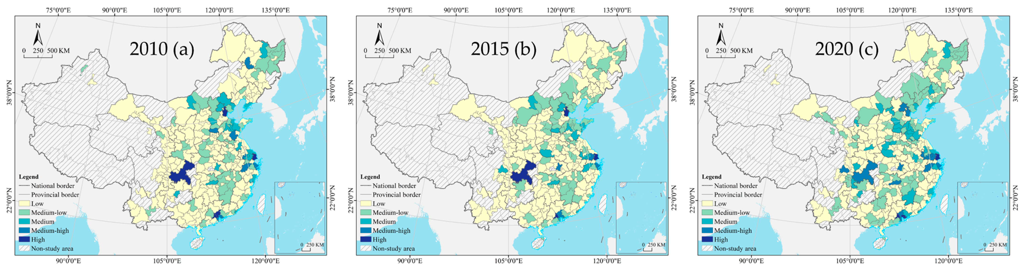
3.2.1. Mismatch Types and Contribution of GDP

The supply mismatch of UPGS in China is relatively stable in terms of types, dominated by negative matching, to a moderate extent. In 2010, positive mismatch, positive matching, negative matching, negative mismatch cities accounted for 9%, 24%, 49%, 18%, respectively, while accounting for 7%, 26%, 48%, 20% in 2015, and 7%, 22%, 49%, 22% in 2020. Positive mismatch cities were in the minority, spread out in a scattered pattern in the east-central and western regions, and shrinking further towards the east and central parts. Positive and negative matching cities were clustered in most of the country. Negative mismatch cities were clustered in blocks in the Beijing-Tianjin-Hebei region, northeast and southwest China, as well as in parts of Shandong, Henan, and Jiangxi, and were further clustered in the Beijing-Tianjin-Hebei region, northeast China, and Shandong (Figure 6).

The contribution of the mismatch in the supply of UPGS in China showed the spatial characteristics of evolution from coastal to inland areas and presented an obvious block aggregation law. In 2010, high, medium-high, medium, medium-low, and low cities accounted for 1.75%, 2.80%, 6.99%, 19.23%, and 68.53%, respectively, while accounting for 1.40%, 1.75%, 5.59%, 23.43%, 67.48% in 2015, and 1.40%, 4.55%, 10.84%, 27.97%, 54.20% in 2020. A small number of high and medium-high cities were there, increasing only from 13 in 2010 to 17 in 2020. Medium cities were scattered in distribution, and gradually spread from the east to the west and central parts of the country. Medium-low cities were clustered in blocks, mainly in the east and central parts and the northeast and spread further to the northwest and southwest. Low cities were scattered throughout most of the country, but they shrank slightly at different stages (Figure 7).

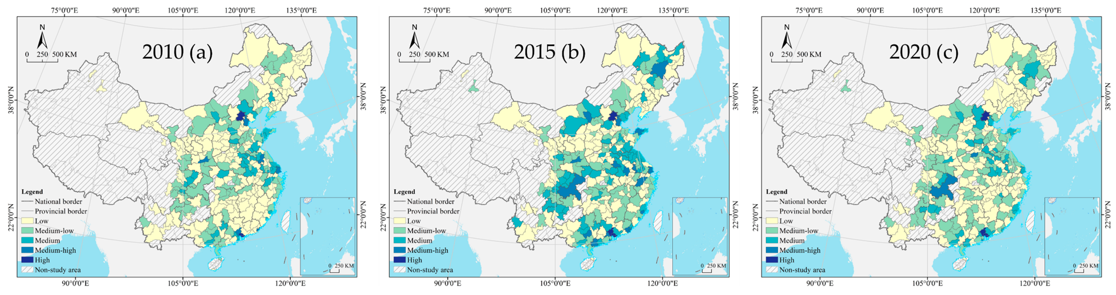
3.2.2. Mismatch Types and Contribution of Population

The demand mismatch of UPGS in China is also relatively stable in terms of types, dominated by positive matching, to a moderate extent. In 2010, positive mismatch, positive matching, negative matching, negative mismatch cities accounted for 21%, 43%, 27%, and 9%, respectively, while accounting for 26%, 40%, 28%, 6% in 2015, and 24%, 41%, 29%, 6% in 2020. Positive mismatch cities were distributed in blocks in the Yangtze River Basin and some parts of Guangdong and Guangxi, and further extend to the Beijing-Tianjin-Hebei region, northeast China, and Sichuan. Positive matching cities were clustered in most of the country. The agglomerations of negative matching cities shifted from the Beijing-Tianjin-Hebei region, southwest and northeast China as well as Jiangxi and Guangdong to the Beijing-Tianjin-Hebei region, the Shandong Peninsula, northeast and northwest China as well as Hunan and Jiangxi. Negative mismatch cities were mainly in the central and eastern regions and gradually shrank (Figure 8).

The demand mismatch contribution of UPGS in China was also obviously clustered in blocks, and gradually developed from the coast to inland. In 2010, high, medium-high, medium, medium-low, and low cities accounted for 1.40%, 1.7%, 12.23%, 27.27% and 57.34%, respectively, while accounting for 1.40%, 1.75%, 20.98%, 25.52%, 44.76% in 2015, and 1.40%, 1.04%, 11.19%, 33.22%, 52.80% in 2020. There was a small number of high and medium-high cities, decreasing from nine in 2010 to seven in 2020. Medium cities were scattered in the Beijing-Tianjin-Hebei and Yangtze River Delta regions, as well as some parts in Sichuan, Guangdong, and Guangxi. Medium-low cities were clustered in blocks, expanding further from the central and eastern, southwestern, and northeastern regions to the southwest, northeast, and southeast. Low cities were scattered throughout most of the country, with slight shrinking (Figure 9).

3.3. Driving Factors of Urban Green Space

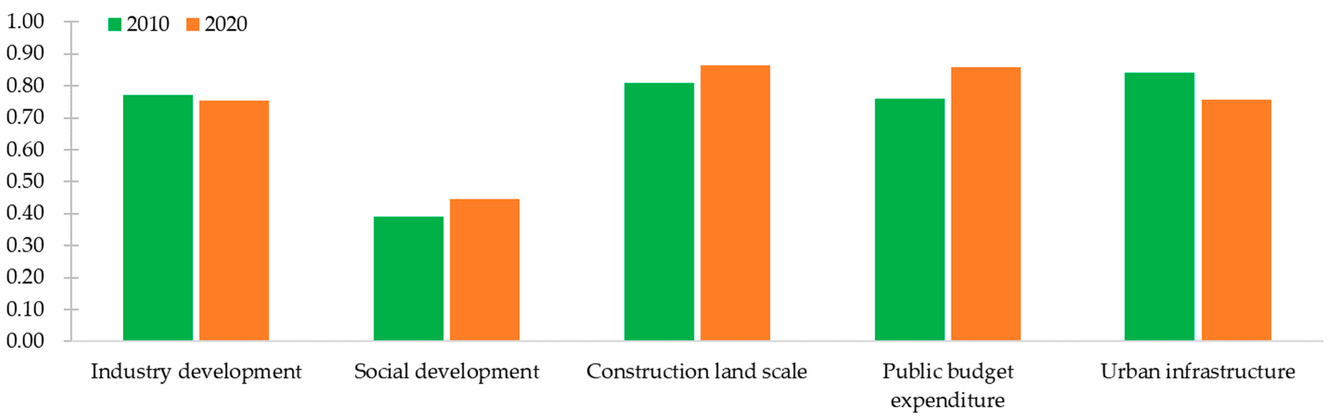
3.3.1. Factor Detection

The direct and interactive influencing factors of UPGS in China were calculated by running Geodetector in the R language (

Table 4. Result of factor detection of UPGS, all q-values passed the 99% significance test.

Type	${\mathit{X}}_{\mathit{i}}$	2010		2020
		q-Value	p-Value	q-Value	p-Value
Industry development	$X_1$	0.69 ***	0.00	0.78 ***	0.00
	$X_2$	0.85 ***	0.00	0.73 ***	0.00
Social development	$X_3$	0.29 ***	0.00	0.34 ***	0.00
	$X_4$	0.49 ***	0.00	0.55 ***	0.00
Construction land scale	$X_5$	0.82 ***	0.00	0.87 ***	0.00
	$X_6$	0.79 ***	0.00	0.85 ***	0.00
Public budget expenditure	$X_7$	0.75 ***	0.00	0.82 ***	0.00
	$X_8$	0.76 ***	0.00	0.89 ***	0.00
Urban infrastructure	$X_9$	0.84 ***	0.00	0.75 ***	0.00
	$X_{10}$	0.84 ***	0.00	0.77 ***	0.00

Note: *** stands for p < 0.01.

,

Table 5. Result of interaction detection of UPGS in 2010, underlined fonts are single-line weakening, others are bilinear enhancement.

	$X_1$	$X_2$	$X_3$	$X_4$	$X_5$	$X_6$	$X_7$	$X_8$	$X_9$	$X_{10}$
$X_1$	0.69
$X_2$	0.86	0.85
$X_3$	0.79	0.91	0.29
$X_4$	0.69	0.88	0.71	0.49
$X_5$	0.81	0.91	0.93	0.85	0.82
$X_6$	0.88	0.94	0.91	0.84	0.82	0.79
$X_7$	0.77	0.88	0.90	0.81	0.88	0.87	0.75
$X_8$	0.85	0.90	0.84	0.83	0.87	0.86	0.80	0.76
$X_9$	0.85	0.91	0.91	0.90	0.90	0.91	0.87	0.89	0.84
$X_{10}$	0.90	0.92	0.91	0.86	0.88	0.87	0.89	0.88	0.94	0.84

and

Table 6. Result of interaction detection of UPGS in 2020, underlined fonts are single-line weakening, others are bilinear enhancement.

	$X_1$	$X_2$	$X_3$	$X_4$	$X_5$	$X_6$	$X_7$	$X_8$	$X_9$	$X_{10}$
$X_1$	0.69
$X_2$	0.89	0.85
$X_3$	0.77	0.83	0.29
$X_4$	0.91	0.86	0.69	0.49
$X_5$	0.92	0.87	0.86	0.89	0.82
$X_6$	0.90	0.85	0.87	0.89	0.89	0.79
$X_7$	0.90	0.87	0.82	0.87	0.91	0.90	0.75
$X_8$	0.90	0.91	0.89	0.90	0.95	0.93	0.90	0.76
$X_9$	0.89	0.83	0.83	0.81	0.88	0.87	0.89	0.93	0.84
$X_{10}$	0.90	0.78	0.81	0.82	0.88	0.86	0.89	0.93	0.87	0.84

), and all independent variables in factor detection passed a 99% significance test. It shows significant variation in the forces of the independent variables, with great changes in the strong-acting factors. In 2010, the factors had a minimum force of 0.29, a maximum value of 0.84, and an average value of 0.71; the output value of the tertiary industry ($X_2$), area of land used for urban construction ($X_5$), area of city paved roads ($X_9$), and number of buses and trolley buses under operation ($X_{10}$) acted as strong acting factors with a force greater than 0.8. In 2020, the factors had a minimum force of 0.34, a maximum value of 0.89, and an average value of 0.74; the area of land used for urban construction ($X_5$), area of land used for living ($X_6$), local general public budget expenditure ($X_7$), and education expenditure in local general public budget ($X_8$) acted as strong acting factors with a force greater than 0.8.

The mean of the five types of independent variable driving factors was calculated (Figure 10). It shows that the strength and ranking of different types of driving forces fluctuated somewhat in both years. In 2012, the driving forces had a minimum value of 0.39, a maximum value of 0.84, and an average value of 0.71, with the social development factor being the weakest and the urban infrastructure factor the strongest. In 2020, the driving forces had values ranging from a minimum of 0.45 to a maximum of 0.86, with an average of 0.74, with the social development factor the weakest, and the construction land scale factor the strongest.

3.3.2. Interaction Detection

The interaction detection effects were wholly dependent on bilinear enhancement, with a small amount of unilinear weakening, a large interaction force and great changes in the super-interaction factors. In 2010, the interaction forces had values ranging from a minimum of 0.69 to a maximum of 0.94, with an average of 0.87, with the interaction forces of $X_9\cap X_{10}$, $X_2\cap X_6$, $X_3\cap X_5$, $X_2\cap X_{10}$, $X_3\cap X_{10}$, $X_2\cap X_9$, $X_2\cap X_5$, $X_3\cap X_9$, $X_6\cap X_9$, $X_2\cap X_3$ and $X_3\cap X_6$ being greater than 0.9. The factors output value of the tertiary industry ($X_2$) and population urbanization rate ($X_3$) appeared most frequently and they were considered as super interaction factors. In 2020, the interaction forces had had values ranging from a minimum of 0.69 to a maximum of 0.95, with an average of 0.87, with the interaction forces of $X_5\cap X_8$, $X_8\cap X_{10}$, $X_6\cap X_8$, $X_8\cap X_9$, $X_1\cap X_5$, $X_2\cap X_8$, $X_5\cap X_7$ and $X_1\cap X_4$ being greater than 0.9. The factor education expenditure in the local general public budget ($X_8$) appeared most frequently and it was considered as a super interaction factor.

4. Discussion

4.1. Spatial Chracteristics

It was found that UPGS in China presented a very obvious coastal-inland gradient difference, and block-like aggregation in some areas, prominently characterized by spatial differentiation. In the available studies, Huang et al. explained that the overall availability of green space in Southeast, Central and Northeast China is higher, and the availability of green space is generally higher in developed cities than in less developed cities [41]. Duan et al. stated that the average urban forest coverage in China is 19.7%, with obvious differences between northern and southern cities [62]. Dou et al. pointed out that China’s mega-cities have the highest proportion of green space, while large, medium and small-sized cities have a lower proportion of green space [63]. Yang et al. pointed out that the overall green space quality of Chinese cities is at an intermediate level, with western and northeastern China higher than eastern and central China, and that the green space quality of mega-cities, megalopolises, and small cities is higher than that of large and medium-sized cities [42]. Wu et al. argued that long-term built-up areas, newly built-up areas, and non-built-up areas in 107 cities in China are clearly different in long-term greening trends [64]. Hong et al. stated that the greening coverage, greening stability, and greening balance in the core built-up areas of 319 cities were higher in the south but lower in the north, with narrowing regional differences [65]. Long et al. pointed out that most of the 4353 cities in the world have high green space accessibility, with cities with lower accessibility mainly located in South America, Africa, and Asia [14]. Kabisch et al. stated that green space availability in southern European cities is overall lower than in northern European cities [15]. Zepp et al. explained that there were large differences in the share, structure, and green space accessibility in eight European metropolitan areas [66]. Richards et al. pointed out that green space coverage varies greatly among cities in Southeast Asia, with cities having larger land areas and higher population densities characterized by obviously lower green space coverage [19]. The conclusions reached in this study largely coincide with their findings, indicating that spatial imbalance of UPGS (green land) are geographic phenomena prevalent in different countries.

This paper also showed that the mismatch between the supply and demand of UPGS in China was relatively stable to a moderate extent and presented the same obvious spatial heterogeneity. Existing studies have explored the supply and demand of UPGS at a macro scale. Song et al. stated that the overall difference in UPGS supply and demand in China has obviously converged, and that the low per capita area of some small and medium-sized cities in the northeast and central and western regions is a key obstacle to the improvement of the overall supply and demand [9]. Some studies focus on the urban scale, for example, Schrammeijer et al. stated that there are obvious differences in the demand for the four functions of relaxation, cooling, socializing, and walking in UPGS among residents of Amsterdam (Netherlands), and that there is a high degree of mismatch between the demand for and supply of the relaxation and cooling functions [67]. Baró et al. pointed out that the supply and demand for ecosystem services of UPGS in five European cities were highly heterogeneous [68]. Fusaro et al. found that the mismatch of ecosystem services is more severe in cities in northern Italy than in the south [69]. Hao et al. pointed out that the supply and demand of UPGS in the second and third ring road areas of Changchun (China) is well matched, and the imbalance is concentrated in the development areas within the first ring road and in the outskirts of the city [70]. Shi et al. argued that the supply and demand system of UPGS in Zhengzhou (China) is generally characterized by a low level of coordination and a supply lag, and there is a mismatch of supply and demand between the old and new urban areas [71]. In addition, this paper and they both identified the mismatch between the supply and demand of UPGS, but there were differences in the degree of mismatch derived due to the different research indicators and methods. In contrast, this paper analyzed the matching of UPGS in two dimensions of supply (GDP) and demand (population), and also explored the mismatch types, better facilitating the government to perform management work.

4.2. Driving Mechanism

This paper found that the driving factors of UPGS in China were diversified, and the driving strengths of the five types of factors showed large differences, and the strong-acting factor and super-interacting factor changed significantly in two years. In the existing studies, Song et al. held that there is a negative effect of land development on the mismatch of UPGS in China, and a positive effect of industrial structure, residential land use, public finance, and transportation facilities [9]. Wu et al. stated that economic development, geographic features, and urbanization obviously affect the green space availability for urban residents in China [72]. Li et al. held that climate, urban topography, proportion of secondary industry, and title incentive factors obviously affect the equity of green space in Chinese cities [13]. Huang et al. argued that socio-economic, infrastructure, and geographic environment factors have a big impact on the availability of green space in Chinese cities [41]. Wu et al. pointed out that GDP per capita, population density, and built-up land area have an obvious effect on the equity of use of UPGS in China [10]. Richards et al. explained that the amount of green space in Southeast Asian cities is negatively correlated with population density and positively correlated with GDP per capita [19]. Nor et al. identified spatial structure and population density as the main factors influencing green space changes in three cities in Southeast Asia [73]. Wen et al. identified economic income, ethnic composition as key factors influencing green space availability in American communities [74]. Wüstemann et al. identified income, age, education, and children in the family as closely related to green space provision in German cities [17]. Girma et al. identified built-up area expansion, population growth, and lax planning enforcement as important factors influencing green space availability in Sebeta (Ethiopia) [75]. Vîlcea et al. explained that population density is the main factor influencing the equity of green space distribution in Craiova (Romania) [76]. Zhu et al. pointed out that urbanization in Xiamen (China) is positively correlated with the supply of green space, and the spatial relationship between the two is obviously heterogeneous [77]. Yang et al. stated that age, education, and housing size are all closely related to green space inequality among residents in Guangzhou (China) [43]. Li et al. pointed out that the socio-economic disadvantage index (including wealth, occupation, education, and housing) is closely related to the availability of parkland in Shanghai, and that the abundance and accessibility of parkland are worse in places with higher socio-economic disadvantages [78]. The conclusions of this paper are almost in line with their findings, but the above papers only explored the influence of some factors on UPGS (green land). In contrast, the variables and factors in this study are more comprehensive, and they were further extended to explore the interaction between the variables and their changes, to draw more precise conclusions, which will help the government to perform management in a more refined manner.

4.3. Policy Enlightenment

Based on the policy zoning framework proposed in the previous text, the zoning map for UPGS of China’s 286 cities in 2020 was classified (Figure 11), with a proposal of corresponding development suggestions. According to the zoning results, smart shrinking zones, smart growing zones, status quo zones, and overlay policy zones accounted for 23%, 19%, 52%, and 6%, respectively. Smart shrinking zones were concentrated in the Yangtze River Delta and the Pearl River Delta, with scattered distributions in southwest, northeast, and central China; smart growing zones were concentrated in Inner Mongolia, Liaoning, and Shandong, with scattered distributions in the northeast, southwest, and the Pearl River Delta; status quo zones were distributed across most of the country, while overlay policy zones were scattered in some of the central provinces, as well as in Beijing, Shanghai, and Chongqing.

The smart shrinking zone, smart growing zone, and overlay policy zone are the focus of policy design. For the smart shrinking zone, the timing of park green space construction should be rationalized to control or reduce capital investment. It should control the supply and approval of land and suspend the construction of those already approved. It should encourage improvements in the quality of established park green land rather than authorize new additions. For the smart growing zone, it should raise funds for park green space construction through a variety of channels, accelerate land supply and approval, and relax access conditions. In the renovation areas, incentives should be given to encourage the prioritization of some land into UPGS. For the overlay policy zone, it should, on the basis of making good arrangements for the construction schedule, land use approval, and funding of local UPGS, emphasize regional cooperation and adjust the funding for the construction of UPGS in the form of transferring support funds, thus regulating the construction process.

5. Conclusions

The construction of UPGS must match the urban economic development and population size, and mismatch analysis and evaluation are prerequisites for the optimal allocation of UPGS resources. Focusing on large spatio-temporal scales, this paper constructed an integrated technical framework of UPGS, including “evolution mode + supply–demand matching + driving factors + policy zoning”, with an empirical study of 286 Chinese cities. The findings are as follows:

(1)

UPGS in China was in a stable spatial pattern, showing generally the spatial characteristics of coastal-inland gradient difference and block-like aggregation in some areas. The number of cities with four types of evolution modes remained stable, showing a “pyramid” structure, ranked as booming green cities > developing green cities > steady green cities > limited green cities, with the cities showing better evolution in the central and eastern regions, as well as in the major provincial capitals and key cities;

(2)

The supply–demand mismatch of UPGS in China remained stable in type to a moderate extent, with supply mismatch dominated by negative matching, and demand mismatch dominated by positive matching. The contribution of supply and demand mismatches similarly showed a distribution pattern of gradual decrease from coast to inland and the aggregation of blocks in some areas;

(3)

There were differences in the driving factors of UPGS in China, with the factor of social development always being weak and the strong factor changing from urban infrastructure to construction land scale. The interaction detection was dominated by a bilinear enhancement, with super-interaction factors changing from output value of the tertiary industry and population urbanization rate to education expenditure in local general public budget;

(4)

The 286 cities were grouped into four policy zonings for UPGS based on the types of mismatch between supply and demand in China. The smart shrinking zone should implement smart shrinking strategies for UPGS, the smart growing zone should implement smart growing strategies, the status quo zone should maintain status quo development strategies, and the overlay policy zone should implement shrinking or growing strategies as appropriate.

Theoretically, this paper analyzed the UPGS supply and demand from the two perspectives of GDP and population, and introduced the spatial mismatch model into the calculation of the supply–demand relationship, thus further expanding the calculation indices and methods. This paper also analyzed the direct and interactive influences on the spatial differentiation of UPGS using Geodetector, making it the first attempt to perform multi-indicator integrated exploration at a macro scale. In practice, this paper proposed the integrated composite technical framework of “evolution mode + supply–demand matching + driving factors + policy zoning”, effectively connecting the theoretical analysis of UPGS and its practical application, and thereby providing a simple and easy-to-implement technical method for the planning of UPGS at a large scale, which is also applicable to the previously mentioned countries in Europe, the Americas, and Southeast Asia.

Nevertheless, some shortcomings also exist. First of all, the supply–demand relationship was presented based on the urban GDP and population alone. However, there are many urban elements in close connection the UPGS supply and demand, such as financial expenditures, land for construction, and people of different age groups. Therefore, it is necessary to further subdivide and supplement the indicators. Secondly, UPGS showed an obvious spatial heterogeneity, but due to the limitation of space, this paper did not analyze the spatial heterogeneity law of the influencing factors in depth. Therefore, the influencing mechanisms can be further explored in depth based on Geodetector and geographically weighted regression.

References

- Kabisch, N.; Haase, D. Green justice or just green? Provision of urban green spaces in Berlin, Germany. Landsc. Urban Plan. 2014, 122, 129–139. [Google Scholar] [CrossRef]
- Reyes-Riveros, R.; Altamirano, A.; De La Barrera, F.; Rozas-Vásquez, D.; Vieli, L.; Meli, P. Linking public urban green spaces and human well-being: A systematic review. Urban For. Urban Green. 2021, 61, 127105. [Google Scholar] [CrossRef]
- Wolch, J.R.; Byrne, J.; Newell, J.P. Urban green space, public health, and environmental justice: The challenge of making cities ‘just green enough’. Landsc. Urban Plan. 2014, 125, 234–244. [Google Scholar] [CrossRef]
- Şenik, B.; Uzun, O. A process approach to the open green space system planning. Landsc. Ecol. Eng. 2022, 18, 203–219. [Google Scholar] [CrossRef]
- Ministry of Housing and Urban-Rural Development of the People’s Republic of China (MHURD). Standard for Planning of Urban Green Space. Available online: https://www.mohurd.gov.cn/gongkai/zhengce/zhengcefilelib/201910/20191012_242194.html (accessed on 17 July 2023).
- Chen, Y.; Yue, W.; La Rosa, D. Which communities have better accessibility to green space? An investigation into environmental inequality using big data. Landsc. Urban Plan. 2020, 204, 103919. [Google Scholar] [CrossRef]
- Xing, L.; Liu, Y.; Liu, X.; Wei, X.; Mao, Y. Spatio-temporal disparity between demand and supply of park green space service in urban area of Wuhan from 2000 to 2014. Habitat Int. 2018, 71, 49–59. [Google Scholar] [CrossRef]
- National Bureau of Statistics of People’s Republic of China (NBS). In China Urban Construction Statistical Yearbook; NBS: Beijing, China, 2020.
- Song, Y.; He, C.; Xu, Y.; Qu, J. Spatio-temporal evolution and driving mechanism of supply and demand of urban park green space in China. J. Nat. Resour. 2023, 38, 1194–1209. [Google Scholar] [CrossRef]
- Wu, L.; Kim, S.K. Exploring the equality of accessing urban green spaces: A comparative study of 341 Chinese cities. Ecol. Indic. 2021, 121, 107080. [Google Scholar] [CrossRef]
- Huang, Y.; Lin, T.; Zhang, G.; Jones, L.; Xue, X.; Ye, H.; Liu, Y. Spatiotemporal patterns and inequity of urban green space accessibility and its relationship with urban spatial expansion in China during rapid urbanization period. Sci. Total Environ. 2022, 809, 151123. [Google Scholar] [CrossRef]
- Wu, L.; Kim, S.K.; Lin, C. Socioeconomic groups and their green spaces availability in urban areas of China: A distributional justice perspective. Environ. Sci. Policy 2022, 131, 26–35. [Google Scholar] [CrossRef]
- Li, X.; Ma, X.; Hu, Z.; Li, S. Investigation of urban green space equity at the city level and relevant strategies for improving the provisioning in China. Land Use Policy 2021, 101, 105144. [Google Scholar] [CrossRef]
- Long, X.; Chen, Y.; Zhang, Y.; Zhou, Q. Visualizing green space accessibility for more than 4,000 cities across the globe. Environ. Plan. B: Urban Anal. City Sci. 2022, 49, 1578–1581. [Google Scholar] [CrossRef]
- Kabisch, N.; Strohbach, M.; Haase, D.; Kronenberg, J. Urban green space availability in European cities. Ecol. Indic. 2016, 70, 586–596. [Google Scholar] [CrossRef]
- Wolff, M.; Scheuer, S.; Haase, D. Looking beyond boundaries: Revisiting the rural-urban interface of green space accessibility in Europe. Ecol. Indic. 2020, 113, 106245. [Google Scholar] [CrossRef]
- Wüstemann, H.; Kalisch, D.; Kolbe, J. Access to urban green space and environmental inequalities in Germany. Landsc. Urban Plan. 2017, 164, 124–131. [Google Scholar] [CrossRef]
- Huang, C.; Yang, J.; Lu, H.; Huang, H.; Yu, L. Green spaces as an indicator of urban health: Evaluating its changes in 28 mega-cities. Remote Sens. 2017, 9, 1266. [Google Scholar] [CrossRef]
- Richards, D.R.; Passy, P.; Oh, R.R.Y. Impacts of population density and wealth on the quantity and structure of urban green space in tropical Southeast Asia. Landsc. Urban Plan. 2017, 157, 553–560. [Google Scholar] [CrossRef]
- Gupta, K.; Roy, A.; Luthra, K.; Maithani, S.; Mahavir. GIS based analysis for assessing the accessibility at hierarchical levels of urban green spaces. Urban For. Urban Green. 2016, 18, 198–211. [Google Scholar] [CrossRef]
- Mayen Huerta, C. Rethinking the distribution of urban green spaces in Mexico City: Lessons from the COVID-19 outbreak. Urban For. Urban Green. 2022, 70, 127525. [Google Scholar] [CrossRef]
- Sikorska, D.; Łaszkiewicz, E.; Krauze, K.; Sikorski, P. The role of informal green spaces in reducing inequalities in urban green space availability to children and seniors. Environ. Sci. Policy 2020, 108, 144–154. [Google Scholar] [CrossRef]
- Xu, C.; Haase, D.; Pauleit, S. The impact of different urban dynamics on green space availability: A multiple scenario modeling approach for the region of Munich, Germany. Ecol. Indic. 2018, 93, 1–12. [Google Scholar] [CrossRef]
- Xu, C.; Haase, D.; Pribadi, D.O.; Pauleit, S. Spatial variation of green space equity and its relation with urban dynamics: A case study in the region of Munich. Ecol. Indic. 2018, 93, 512–523. [Google Scholar] [CrossRef]
- Fan, P.; Xu, L.; Yue, W.; Chen, J. Accessibility of public urban green space in an urban periphery: The case of Shanghai. Landsc. Urban Plan. 2017, 165, 177–192. [Google Scholar] [CrossRef]
- Cetin, M. Using GIS analysis to assess urban green space in terms of accessibility: Case study in Kutahya. Int. J. Sustain. Dev. World Ecol. 2015, 22, 420–424. [Google Scholar] [CrossRef]
- Ye, C.; Hu, L.; Li, M. Urban green space accessibility changes in a high-density city: A case study of Macau from 2010 to 2015. J. Transp. Geogr. 2018, 66, 106–115. [Google Scholar] [CrossRef]
- Wen, C.; Albert, C.; Von Haaren, C. Equality in access to urban green spaces: A case study in Hannover, Germany, with a focus on the elderly population. Urban For. Urban Green. 2020, 55, 126820. [Google Scholar] [CrossRef]
- Liu, D.; Kwan, M.-P.; Kan, Z. Analysis of urban green space accessibility and distribution inequity in the city of Chicago. Urban For. Urban Green. 2021, 59, 127029. [Google Scholar] [CrossRef]
- Zhang, L.; Chen, P.; Hui, F. Refining the accessibility evaluation of urban green spaces with multiple sources of mobility data: A case study in Shenzhen, China. Urban For. Urban Green. 2022, 70, 127550. [Google Scholar] [CrossRef]
- Li, X.; Huang, Y.; Ma, X. Evaluation of the accessible urban public green space at the community-scale with the consideration of temporal accessibility and quality. Ecol. Indic. 2021, 131, 108231. [Google Scholar] [CrossRef]
- Ma, F. Spatial equity analysis of urban green space based on spatial design network analysis (sDNA): A case study of central Jinan, China. Sustain. Cities Soc. 2020, 60, 102256. [Google Scholar] [CrossRef]
- Ghasemi, K.; Behzadfar, M.; Borhani, K.; Nouri, Z. Geographic information system based combined compromise solution (CoCoSo) method for exploring the spatial justice of accessing urban green spaces, a comparative study of district 22 of Tehran. Ecol. Indic. 2022, 144, 109455. [Google Scholar] [CrossRef]
- Pinto, L.V.; Ferreira, C.S.S.; Inácio, M.; Pereira, P. Urban green spaces accessibility in two European cities: Vilnius (Lithuania) and Coimbra (Portugal). Geogr. Sustain. 2022, 3, 74–84. [Google Scholar] [CrossRef]
- Buckland, M.; Pojani, D. Green space accessibility in Europe: A comparative study of five major cities. Eur. Plan. Stud. 2023, 31, 146–167. [Google Scholar] [CrossRef]
- Schindler, M.; Le Texier, M.; Caruso, G. How far do people travel to use urban green space? A comparison of three European cities. Appl. Geogr. 2022, 141, 102673. [Google Scholar] [CrossRef]
- Yang, J.; Duan, C.; Wang, H.; Chen, B. Spatial supply-demand balance of green space in the context of urban waterlogging hazards and population agglomeration. Resour. Conserv. Recycl. 2023, 188, 106662. [Google Scholar] [CrossRef]
- Yang, Z.; Gao, W. Evaluating the coordinated development between urban greening and economic growth in Chinese cities during 2005 to 2019. Int. J. Environ. Res. Public Health 2022, 19, 9596. [Google Scholar] [CrossRef] [PubMed]
- Li, F.; Wang, X.; Liu, H.; Li, X.; Zhang, X.; Sun, Y.; Wang, Y. Does economic development improve urban greening? Evidence from 289 cities in China using spatial regression models. Environ. Monit. Assess. 2018, 190, 541. [Google Scholar] [CrossRef]
- Cheng, M.; Liang, Y.; Zeng, C.; Pan, Y.; Zhu, J.; Wang, J. Economic growth does not mitigate its decoupling relationship with urban greenness in China. Land 2023, 12, 614. [Google Scholar] [CrossRef]
- Huang, Y.; Lin, T.; Xue, X.; Zhang, G.; Liu, Y.; Zeng, Z.; Zhang, J.; Sui, J. Spatial patterns and inequity of urban green space supply in China. Ecol. Indic. 2021, 132, 108275. [Google Scholar] [CrossRef]
- Yang, Z.; Fang, C.; Mu, X.; Li, G.; Xu, G. Urban green space quality in China: Quality measurement, spatial heterogeneity pattern and influencing factor. Urban For. Urban Green. 2021, 66, 127381. [Google Scholar] [CrossRef]
- Yang, W.; Yang, R.; Zhou, S. The spatial heterogeneity of urban green space inequity from a perspective of the vulnerable: A case study of Guangzhou, China. Cities 2022, 130, 103855. [Google Scholar] [CrossRef]
- Zhang, X.Q. The trends, promises and challenges of urbanisation in the world. Habitat Int. 2016, 54, 241–252. [Google Scholar] [CrossRef]
- Guan, X.; Wei, H.; Lu, S.; Dai, Q.; Su, H. Assessment on the urbanization strategy in China: Achievements, challenges and reflections. Habitat Int. 2018, 71, 97–109. [Google Scholar] [CrossRef]
- Zhang, H.; Padullés Cubino, J.; Nizamani, M.M.; Harris, A.J.; Cheng, X.; Da, L.; Sun, Z.; Wang, H. Wealth and land use drive the distribution of urban green space in the tropical coastal city of Haikou, China. Urban For. Urban Green. 2022, 71, 127554. [Google Scholar] [CrossRef]
- Sperandelli, D.I.; Dupas, F.A.; Pons, N.A.D. Dynamics of urban sprawl, vacant land, and green spaces on the metropolitan fringe of São Paulo, Brazil. J. Urban Plan. Dev. 2013, 139, 274–279. [Google Scholar] [CrossRef]
- He, S.; Wu, Y.; Wang, L. Characterizing horizontal and vertical perspectives of spatial equity for various urban green spaces: A case study of Wuhan, China. Front. Public Health 2020, 8, 10. [Google Scholar] [CrossRef]
- Chen, W.Y.; Hu, F.Z.Y.; Li, X.; Hua, J. Strategic interaction in municipal governments’ provision of public green spaces: A dynamic spatial panel data analysis in transitional China. Cities 2017, 71, 1–10. [Google Scholar] [CrossRef]
- Wendel, H.E.W.; Downs, J.A.; Mihelcic, J.R. Assessing equitable access to urban green space: The role of engineered water infrastructure. Environ. Sci. Technol. 2011, 45, 6728–6734. [Google Scholar] [CrossRef]
- Aksoy, S.; Durmusoglu, Y. Improving competitiveness level of Turkish intermodal ports in the frame of green port concept: A case study. Marit. Policy Manag. 2020, 47, 203–220. [Google Scholar] [CrossRef]
- Bernal Escoto, B.E.; Montero Delgado, N.I.; Rivera Aguirre, F.A. Strategic analysis of sustainable tourism in Baja California against COVID-19. Sustainability 2021, 13. [Google Scholar] [CrossRef]
- Kain, J.F. Housing segregation, negro employment, and metropolitan decentralization. Q. J. Econ. 1968, 82, 175–197. [Google Scholar] [CrossRef]
- Glaeser, E.L.; Hausman, N. The spatial mismatch between innovation and joblessness. Innov. Policy Econ. 2020, 20, 233–299. [Google Scholar] [CrossRef]
- Li, G.; Xu, Z.; Wu, C.; Zhuo, Y.; Tong, X.; Wei, Y.; Shen, X. Inside or outside? The impact factors of zoning–land use mismatch. Sustainability 2019, 12. [Google Scholar] [CrossRef]
- Liu, C.Y.; Painter, G. Immigrant settlement and employment suburbanisation in the US: Is there a spatial mismatch? Urban Stud. 2012, 49, 979–1002. [Google Scholar] [CrossRef]
- Theys, T.; Deschacht, N.; Adriaenssens, S.; Verhaest, D. The evolution of inter-regional spatial mismatch in the USA: The role of skills and spatial structure. Urban Stud. 2019, 56, 2654–2669. [Google Scholar] [CrossRef]
- Wang, J.; Xu, C. Geodetector: Principle and prospective. Acta Geogr. Sin. 2017, 72, 116–134. [Google Scholar] [CrossRef]
- Tegegne, A.M.; Lohani, T.K.; Eshete, A.A. Groundwater potential delineation using geodetector based convolutional neural network in the Gunabay watershed of Ethiopia. Environ. Res. 2024, 242, 117790. [Google Scholar] [CrossRef]
- Wang, W.; Samat, A.; Abuduwaili, J.; Ge, Y. Quantifying the influences of land surface parameters on LST variations based on GeoDetector model in Syr Darya Basin, Central Asia. J. Arid Environ. 2021, 186, 104415. [Google Scholar] [CrossRef]
- Zheng, A.; Wang, T.; Li, X. Spatiotemporal characteristics and risk factors of the COVID-19 pandemic in New York State: Implication of future policies. ISPRS Int. J. Geo-Inf. 2021, 10. [Google Scholar] [CrossRef]
- Duan, Q.; Tan, M. Using a geographical detector to identify the key factors that influence urban forest spatial differences within China. Urban For. Urban Green. 2020, 49, 126623. [Google Scholar] [CrossRef]
- Dou, Y.; Kuang, W. A comparative analysis of urban impervious surface and green space and their dynamics among 318 different size cities in China in the past 25 years. Sci. Total Environ. 2020, 706, 135828. [Google Scholar] [CrossRef]
- Wu, W.; Ma, J.; Meadows, M.E.; Banzhaf, E.; Huang, T.; Liu, Y.; Zhao, B. Spatio-temporal changes in urban green space in 107 Chinese cities (1990–2019): The role of economic drivers and policy. Int. J. Appl. Earth Obs. Geoinf. 2021, 103, 102525. [Google Scholar] [CrossRef]
- Hong, C.; Jin, X. Green change in the core build-up areas of China: Information from MODIS data. Ecol. Indic. 2021, 122, 107270. [Google Scholar] [CrossRef]
- Zepp, H.; Groß, L.; Inostroza, L. And the winner is? Comparing urban green space provision and accessibility in eight European metropolitan areas using a spatially explicit approach. Urban For. Urban Green. 2020, 49, 126603. [Google Scholar] [CrossRef]
- Schrammeijer, E.A.; Malek, Ž.; Verburg, P.H. Mapping demand and supply of functional niches of urban green space. Ecol. Indic. 2022, 140, 109031. [Google Scholar] [CrossRef]
- Baró, F.; Haase, D.; Gómez-Baggethun, E.; Frantzeskaki, N. Mismatches between ecosystem services supply and demand in urban areas: A quantitative assessment in five European cities. Ecol. Indic. 2015, 55, 146–158. [Google Scholar] [CrossRef]
- Fusaro, L.; Nardella, L.; Manes, F.; Sebastiani, A.; Fares, S. Supply and demand mismatch analysis to improve regulating ecosystem services in Mediterranean urban areas: Insights from four Italian Municipalities. Ecol. Indic. 2023, 155, 110928. [Google Scholar] [CrossRef]
- Hao, L.; Zhang, H.; Zhang, S. Spatial accessibility of urban green space in central area of Changchun: An analysis based on the multi-trip model. Sci. Geogr. Sin. 2021, 41, 695–704. [Google Scholar] [CrossRef]
- Shi, Z.; Xing, L.; Zheng, L.; Mu, B.; Tian, G. Evaluations and optimization strategies of synergy degree of park green space on balance of supply and demand for recreation. J. Nanjing For. Univ. 2021, 45, 197–204. [Google Scholar] [CrossRef]
- Wu, L.; Kim, S.K. How are green spaces distributed among different social groups in urban China? A national level study. Forests 2020, 11, 1317. [Google Scholar] [CrossRef]
- Muhamad Nor, A.N.; Abdul Aziz, H.; Nawawi, S.A.; Muhammad Jamil, R.; Abas, M.A.; Hambali, K.A.; Yusoff, A.H.; Ibrahim, N.; Rafaai, N.H.; Corstanje, R.; et al. Evolution of green space under rapid urban expansion in southeast Asian cities. Sustainability 2021, 13, 2024. [Google Scholar] [CrossRef]
- Wen, M.; Zhang, X.; Harris, C.D.; Holt, J.B.; Croft, J.B. Spatial disparities in the distribution of parks and green spaces in the USA. Ann. Behav. Med. A Publ. Soc. Behav. Med. 2013, 45 (Suppl. S1), S18–S27. [Google Scholar] [CrossRef] [PubMed]
- Girma, Y.; Terefe, H.; Pauleit, S.; Kindu, M. Urban green spaces supply in rapidly urbanizing countries: The case of Sebeta Town, Ethiopia. Remote Sens. Appl. Soc. Environ. 2019, 13, 138–149. [Google Scholar] [CrossRef]
- Vîlcea, C.; Șoșea, C. A GIS-based analysis of the urban green space accessibility in Craiova city, Romania. Geogr. Tidsskr.-Dan. J. Geogr. 2020, 120, 19–34. [Google Scholar] [CrossRef]
- Zhu, Z.; Li, J.; Chen, Z. Green space equity: Spatial distribution of urban green spaces and correlation with urbanization in Xiamen, China. Environ. Dev. Sustain. 2023, 25, 423–443. [Google Scholar] [CrossRef]
- Li, H.; Liu, Y. Neighborhood socioeconomic disadvantage and urban public green spaces availability: A localized modeling approach to inform land use policy. Land Use Policy 2016, 57, 470–478. [Google Scholar] [CrossRef]