
Long-Term Patterns in Forest Soil CO2 Flux in a Pacific Northwest Temperate Rainforest
by
 , , ,
, , ,
Dylan G. Fischer
1,*,
Zoe R. Chamberlain
2,
Claire E. Cook
2,
Randall Adam Martin
3 and
Liam O. Mueller
4 1
Environmental Studies Path, SEM II, The Evergreen State College, Olympia, WA 98505, USA
2
EEON Laboratory, The Evergreen State College, Olympia, WA 98505, USA
3
Ecostudies Institute, P.O. Box 1614, Olympia, WA 98507, USA
4
Department of Molecular Biology, University of California San Diego, San Diego, CA 92093, USA
*
Author to whom correspondence should be addressed.
Forests 2024, 15(1), 161; https://doi.org/10.3390/f15010161
Submission received: 10 December 2023
/
Revised: 5 January 2024
/
Accepted: 10 January 2024
/
Published: 12 January 2024
(This article belongs to the Collection Forests Carbon Fluxes and Sequestration)
Abstract
:Soil CO2 efflux (Fs) plays an important role in forest carbon cycling yet estimates of Fs can remain unconstrained in many systems due to the difficulty in measuring Fs over long time scales in natural systems. It is important to quantify seasonal patterns in Fs through long-term datasets because individual years may show patterns that are not reflective of long-term averages. Additionally, determining predictability of net patterns in soil carbon flux based on environmental factors, such as moisture and temperature, is critical for appropriately modeling forest carbon flux. Ecosystems in moderate climates may have strong CO2 efflux even during winter, and so continuous quantification of annual variability is especially important. Here, we used a 2008–2023 dataset in a lowland temperate forest ecosystem to address two main questions: (1) What are the seasonal patterns in Fs in a highly productive temperate rainforest? (2) How is average Fs across our study area predicted by average coincident temperature, soil moisture and precipitation totals? Data showed clear seasonality where Fs values are higher in summer. We also find Fs across our measurement network was predicted by variation in abiotic factors, but the interaction between precipitation/moisture and temperature resulted in greater complexity. Specifically, in spring a relatively strong relationship between air temperature and Fs was present, while in summer the relationship between temperature and Fs was flat. Winter and autumn seasons showed weak positive relationships. Meanwhile, a negative relationship between precipitation and Fs was present in only some seasons because most precipitation falls outside the normal growing season in our study system. Our data help constrain estimates of soil CO2 fluxes in a temperate rainforest ecosystem at ~14–20 kg C ha−1 day−1 in summer and autumn, and 6.5–10.5 kg C ha−1 day−1 in winter and spring seasons. Together, estimates suggest this highly productive temperate rainforest has annual soil-to-atmosphere fluxes of CO2 that amount to greater than 4.5 Mg C ha−1 year−1. Sensitivity of such fluxes to regional climate change will depend on the balance of Fs determined by autotrophic phenological responses versus heterotrophic temperature and moisture sensitivity. Relatively strong seasonal variation coupled with comparatively weak responses to abiotic variables suggest Fs may be driven largely by seasonal trends in autotrophic respiration. Accordingly, plant and tree responses to climate may have a stronger effect on Fs in the context of climate change than temperature or moisture changes alone.
1. Introduction
Understanding variation in naturally occurring carbon fluxes is vital for better the understanding and management of global carbon budgets [1]. Forest ecosystems are fundamentally important in the global carbon (C) cycle [2,3,4] in both the uptake and release of C. Global rates of CO2 released by soils through both plant (autotroph) respiration and decomposition (heterotrophic respiration) are up to 10 times higher than anthropogenic emissions of CO2 through burning of fossil fuels and represent the dominant form of C release from soils to atmosphere pools [5,6]. Accordingly, even small changes in the release of CO2 from soils can be produce large values compared to other CO2 fluxes [7,8,9]. Estimating soil CO2 efflux (Fs) with greater precision is important in all terrestrial ecosystems [10,11], but especially forest ecosystems where C-flux and storage are large. In systems that contain large quantities of C, small flux changes can represent large C fluxes globally [10]. Temperate rainforests of the Pacific Northwest have the largest soil C stores of belowground carbon of any system in the contiguous United States [12,13], hence, documenting C-flux patterns in these ecosystems is of particular interest.
Multiple studies have described the relationship between Fs and abiotic factors of temperature and moisture worldwide [7,14,15,16,17,18]. Additionally, seasonality of Fs has been evaluated in multiple systems worldwide [8,19]. Interestingly, while forest ecosystems of the Pacific Northwest represent some of the most carbon-dense ecosystems on Earth [2], long-term studies of relationships between Fs and temperature and moisture in the region are relatively few [20,21,22]. Similarly, the seasonality of Fs fluxes in C-dense Pacific Northwest forests is not well understood, principally because mild winter temperatures extend the growing season for dominant conifers (accompanied by relatively high autotrophic and heterotrophic respiration), and dry summers may constrain heterotrophic respiration [23]. Isotopic analyses have also demonstrated interesting patterns where autotrophic versus heterotrophic sources and contributions to total soil CO2 efflux may vary by season [19,22]. Long-term (~6+ years) datasets have demonstrated seasonal patterns where soil CO2 efflux peaks in mature old-growth Pacific Northwest forests in mid to late summer, and strong relationships with temperature are possible during the growing season when moisture levels are neither too wet nor too dry [21]. Similarly, different biomes inherently differ in the strength of climatic signals for seasonal differences. Regardless, temperature, moisture, and vegetation activity all clearly influence soil CO2 efflux, and all can be affected by seasonal variation. Previous work has also demonstrated the importance of vegetation type in influencing Fs through effects on both subterranean autotrophic respiration and litter decomposition [7,14,24,25,26,27,28,29,30,31]. Forests with mixed deciduous and coniferous dominance may also exhibit patterns where Fs correlates with species composition and/or species diversity [30,32,33]. Stand diversity may also provide a stabilizing influence on Fs where diversity is correlated with reduced sensitivity to temperature [34].
Here, we examine two things: (1) average seasonal trends in Fs over a dataset spanning 2008–2023 in a lowland northwestern temperate rainforest in Washington state (USA) co-dominated by both coniferous and deciduous tree species; and (2) predictability of average Fs based-on average air temperature, precipitation and soil temperature and moisture values.
2. Materials and Methods
2.1. Site Description
Our study took place in The Evergreen State College forest reserve, located near Olympia, Washington, USA (47.0719° N, 122.9766° W; [30]; also, see study sites maps provided in Rex et al. [35]). Local climate is characterized by warm, dry summers and wet, temperate winters (https://weather.evergreen.edu/ last accessed 29 August 2022). The forest was last clear-cut between 1937–39 [30,35]), and is currently dominated by Pseudotsuga menziesii (Mirbel) Franco, Alnus rubra Bong., Acer macrophyllum Pursh, and Thuja plicata Donn ex D.Don. Other important, but less-common, species in the forest canopy include Tsuga heterophylla (Raf.) Sarg. and Abies grandis (Douglas ex D. Don) Lindley.
Our measurements were within a long-term permanent plot network designed for the regular measurement of aboveground forest C-flux and storage (EEON; http://sites.evergreen.edu/eeon; last accessed 1 December 2023). The plot network consists of 44 circular 314 m2 plots, arranged systematically on a 250 m grid across 380 ha [35]. The plots are mature lowland temperate rainforests typical of unmanaged forest in lowlands adjacent to the Puget Sound. The stands at this site best match associations in the G237 group (north Pacific red alder-bigleaf maple-Douglas-fir rainforest based on the United States National Vegetation Classification (https://usnvc.org/; last accessed 29 August 2022). Within each plot, all live trees, snags, and down woody debris have been permanently tagged and measured every 1–3 years since 2008. Stand structure is typical of a ~100-year-old closed-canopy forest on the west slope of the Cascades where average tree density is approximately 369 stems ha−1, (26 SE) and median tree diameter at 1.4 m height (DBH) is 34.5, and mean DBH is 41.3 cm (1.3 SE). Canopies are generally closed-canopy with over 80% tree canopy cover. A previous study [30] and measurements since 2008 estimate net aboveground annual C increment (net increases in aboveground biomass C) at ~1.95 Mg C ha−1 year−1, (0.87 SE). Litterfall biomass measurements from 2007/2008 [30] and again in 2014/2015 suggest that litterfall ranges from an average of 2.86 Mg ha−1 year−1 (0.44 SE) in 2007/2008 to 2.45 Mg ha−1 year−1 (0.31 SE) in 2014/2015.
Soils are represented by Alderwood gravelly sandy loam soils (USDA web soil survey; https://websoilsurvey.sc.egov.usda.gov; last accessed 11 November 2021). Sampling in 2014 suggests < 1 kg C m−2 within the litter layer, 2.5 (0.3 SE) kg C m−2 in the top 5 cm of soil, 4.2 (0.0.38 SE) kg C m−2 between 5 and 30 cm depth, and another 2.5 (0.29 SE) kg C m−2 between 30 and 50 cm soil depth (% C declines from 30%–40% in the litter layer, to 8% at the soil surface to 1.3% at 50 cm depth). Soil nitrogen (N) sampling suggests pool sizes of 0.04 (0.01 SE) kg N m−1 in the litter layer and 0.8 (0.42 SE) kg N m−1 in the top 50 cm of soil depth (declining from 0.36% to 0.1% N with depth).
2.2. Weather Data
Weather data in our study were compiled from the PRISM Climate Group climate data explorer (https://prism.oregonstate.edu/; last accessed 16 April 2023). Long-term averages of temperature and precipitation are also available from nearby weather stations, including a permanent weather station at the field site, maintained by The Evergreen State College, (publicly available at https://weather.evergreen.edu/; last accessed 26 November 2023). Similarly, other nearby NOAA cooperative weather stations have provided useful records in temperature and precipitation data through time (e.g., Olympia AP Station, 456114, https://wrcc.dri.edu/, last accessed 16 April 2023). Nevertheless, gaps in data availability at each station coincident with our measurements ultimately made PRISM-based estimates of temperature and precipitation more useful for a multi-year dataset. To validate the usefulness of the PRISM-based estimates, we conducted simple linear regressions for temperature and precipitation data for 60 measurement dates (the first day of each month) for five years during the study where local weather station data and PRISM data were simultaneously available. PRISM data accurately predicted both site-based measurements of daily temperature (r2 = 0.94, p < 0.0001) and annual precipitation (r2 = 0.80, p = 0.0267) several miles away at a long-term NOAA Cooperative Weather station.
2.3. Net Soil CO2 Efflux Measurements
Plots chosen for analysis varied haphazardly through time due to a combination of changing focal plots (focal plots were changed to avoid long-term trampling effects) and inaccessibility of two plots in 2023. We chose 11 plots for soil CO2 efflux (Fs) measurement between 2008–2011. Plots were randomly chosen from the 44 EEON permanent plots [30]. In 2014–2015, we expanded measurements to include ten additional plots within the larger EEON permanent plot network (20 total plots measured in 2014–2015), and nine from the old plots (two plots were unusable due to vandalism and soil trampling). In 2022, eleven plots (the ten new plots plus one randomly chosen plot from the 2008–2014 set) were remeasured, and in 2023, nine of the new plots were remeasured (two plots were again unusable due to accessibility issues). A simple Welch’s t-test of data from the overlapping sets of plots in 2014–2015 confirmed no significant difference between Fs in the old and new sets of plots (p > 0.05; new and old plot means were 2.12 and 2.17 μmol CO2 m−2 s−1, respectively; see below for methods details). Each plot measurement was averaged from four subplots located in each cardinal direction within each EEON plot, resulting in a total averaged set of 1612 plot measurements between 2008–2023.
We used an open-path IRGA (LC-pro+, ADC Bioscientific Ltd., Hoddesdon, UK) for all Fs measurements. The IRGA is attached to a 40.25 cm2 chamber with integrated fan to maintain air flow. Each measurement consisted of an average of three measures taken at two, three, and four minutes after the chamber was placed on the soil. Chamber placement ensured that the chamber was inserted approximately 1 cm below the soil for each measurement, such that there was no air exchange from the sides of the chamber with the surrounding air. Immediately following chamber placement, Fs was monitored to ensure measurements were stable before the measurements could be counted. If the measurements did not stabilize with 0.5 μmol CO2 m−2 s−1 within two minutes, the chamber was lifted, re-positioned, and measurements were restarted.
Diurnal trends in Fs data can influence scaling of Fs to annual values from daytime measurements [36]. We evaluated diurnal trends in the spring 2009, 2011, and 2012. Spring measurement periods were selected since diurnal temperature changes are at their greatest, and both deciduous and coniferous trees are in their active growth season. In each diurnal measurement event (24 h), Fs was repeatedly measured every three hours for eight sub-plots. The purpose of these measures was to determine if 24 h measurements differed significantly from average daytime measurements. Accordingly, an average of daytime measurements was compared (using a simple one-sample t-test) with measurements within the 24 h measurement that were taken during the normal period for Fs measurement throughout the rest of the study (between 1000 and 1500 h). In this comparison, average values over diurnal measurement periods did not differ significantly from daytime measurements (p = 0.551; mean diurnal and daytime measurement were both 1.267 μmol CO2 m−2 s−1).
For a subset of Fs plot measurements between 2014 and 2023 (2014 n = 15; 2015 n = 83; 2022 n = 33, and 2023 n = 10), soil temperature and moisture measurements were taken simultaneously. Soil temperature and moisture were not available for all data, representing a limitation in the current study. This subset included 141 measurements in winter (n = 44), spring (n = 75), and summer (n = 22). Soil temperature was also measured down to 10 cm depth immediately adjacent to the chamber using a digital thermometer. Soil moisture was measured using a lightweight SM150 Portable Soil Moisture probe (Dynamax, Houston, TX, USA).
2.4. Data Analysis
All subplot data were averaged by plot and month of measurements prior to analysis resulting in 402 average Fs measurements between 2008–2023. Monthly plot averages were analyzed using a REML approach using the lme4 package in R [37,38]. Fixed effects in the model included season (autumn, winter, spring, summer) and stand type (conifer, deciduous, mixed conifer, and deciduous). Average air temperature and precipitation totals were treated as continuous effects, and all interactions between season and stand type and season, temperature, and precipitation were included in the model. Year, month, and plot were all treated as random intercept effects in the model. An α value of p < 0.05 was used to denote significance where relevant.
A similar REML model analysis was used for the subset of measurements between 2014 and 2023 which included soil moisture and temperature. In this subset analysis, 141 measurements were included across all plots, during eight months in winter and summer seasons (autumn data was absent) and four years (2014, 2015, 2022, and 2023). Stand type and season were treated as fixed effects, soil moisture and temperature were treated as continuous effects, and year, month, and plot were treated as random intercept effects in the model. As above, R and the lme4 package were used for all analyses and an α value of 0.05 was used to denote significance.
Following the analysis above, a Q10 value was also calculated for significant soil temperature by Fs relationships. The measure Q10 gives an approximate value for the change in respiration associated with a 10 °C change in temperature [1,39]. Briefly, this analysis calculated Q10 within seasons after fitting the equation Fs = a × e(b×t), where a and b represent constants. Q10 is then calculated based on the equation Q10 = e(b×10), reflecting a multiplicative change in the value of Fs following a 10 °C change in temperature.
3. Results
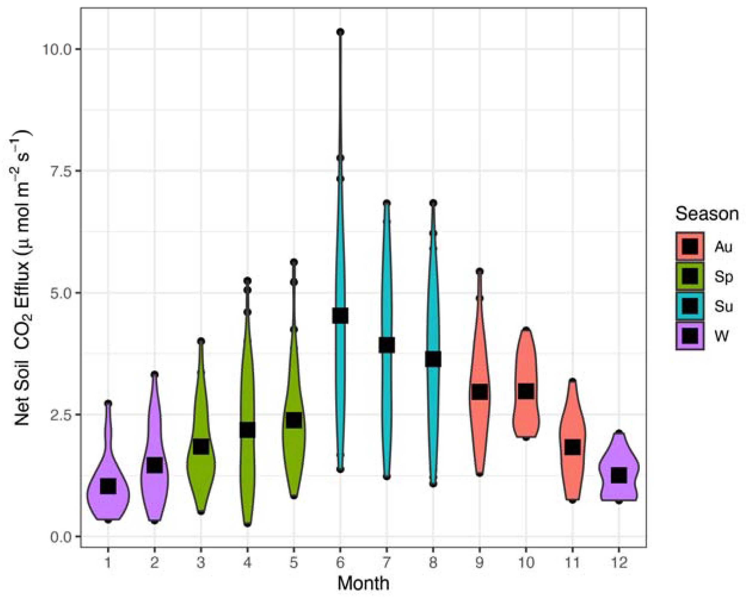
Across all sub-plot measurements between 2008 and 2023, season and average monthly air temperature stood-out as the two strongest single effects in the model (marginal R2 = 0.343, conditional R2 = 0.790), but interaction effects were also significant for season by precipitation, season by air temperature, and season by temperature by precipitation (Table 1). Seasonally, average Fs (μmol CO2 m−2 s−1) was highly variable and peaked rapidly in summer, followed by autumn values, spring, and then winter (Figure 1). The overall average Fs value across all seasons and years was ~2.54 (95% CI: 2.4–2.68 μmol CO2 m−2 s−1). Average Fs in spring was 2.2 (95% CI: 2.03–2.35 μmol CO2 m−2 s−1), average values in autumn were 2.72 (95% CI: 2.53–2.92 μmol CO2 m−2 s−1). Summer averaged 3.92 (95% CI: 3.59–4.25 μmol CO2 m−2 s−1), and winter averaged only 1.25 (95% CI: 1.10–1.40 μmol CO2 m−2 s−1). In the random effects, year accounted for 36.9% of the total variance white plot accounted for only 7.2% (Table S1).
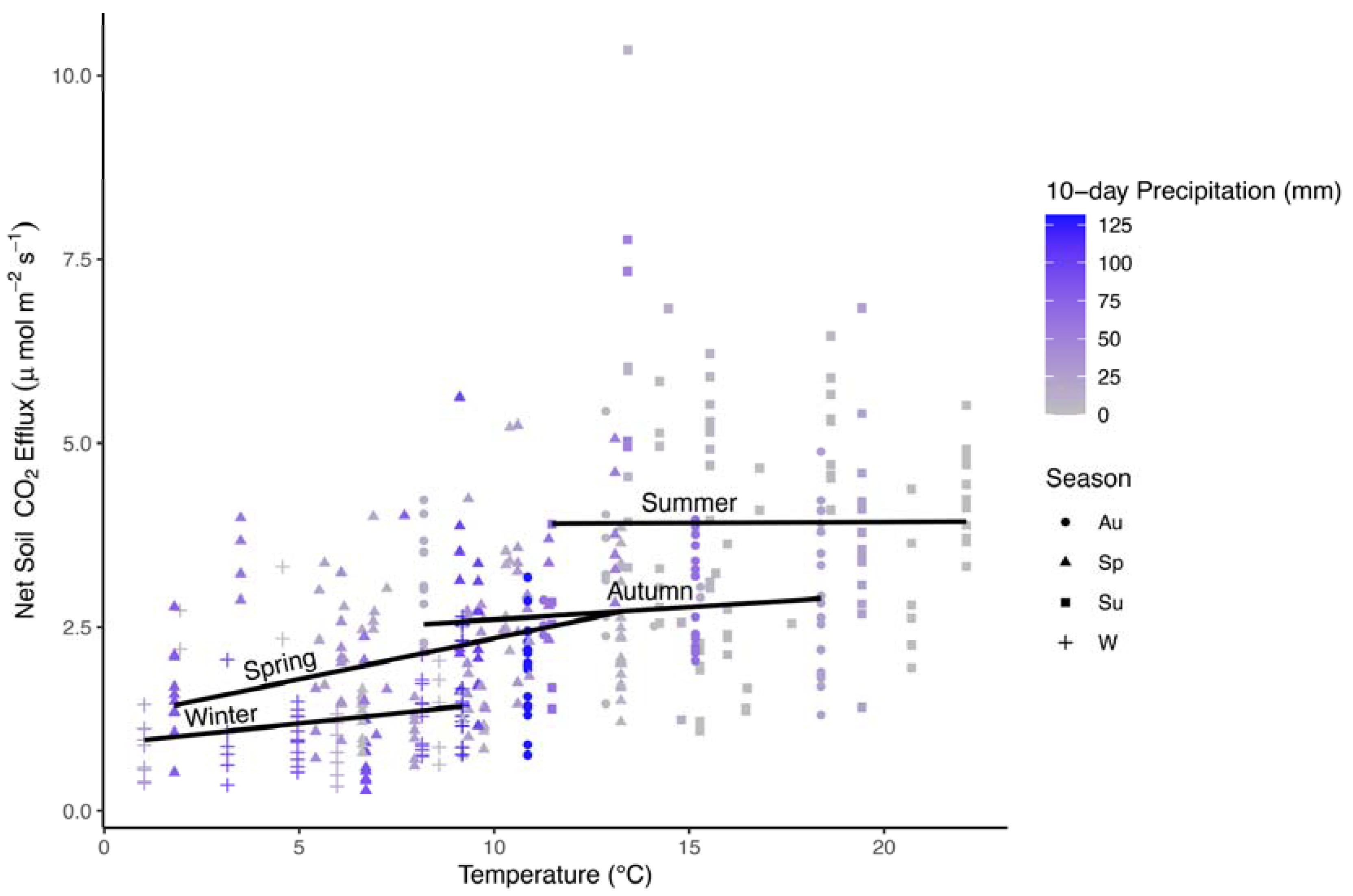
Comparison of the sums of squares (SS) indicated that air temperature alone accounted for ~8% of the variation in SS values, and 48% of the SS values when including all interaction effects (Table 2). Nevertheless, the analysis also suggested significant interactions with season and precipitation such that Fs was similar across a range of air temperatures in summer, showed the strongest positive relationship with air temperature in spring, and was also positively related to temperature in other seasons (Figure 2).
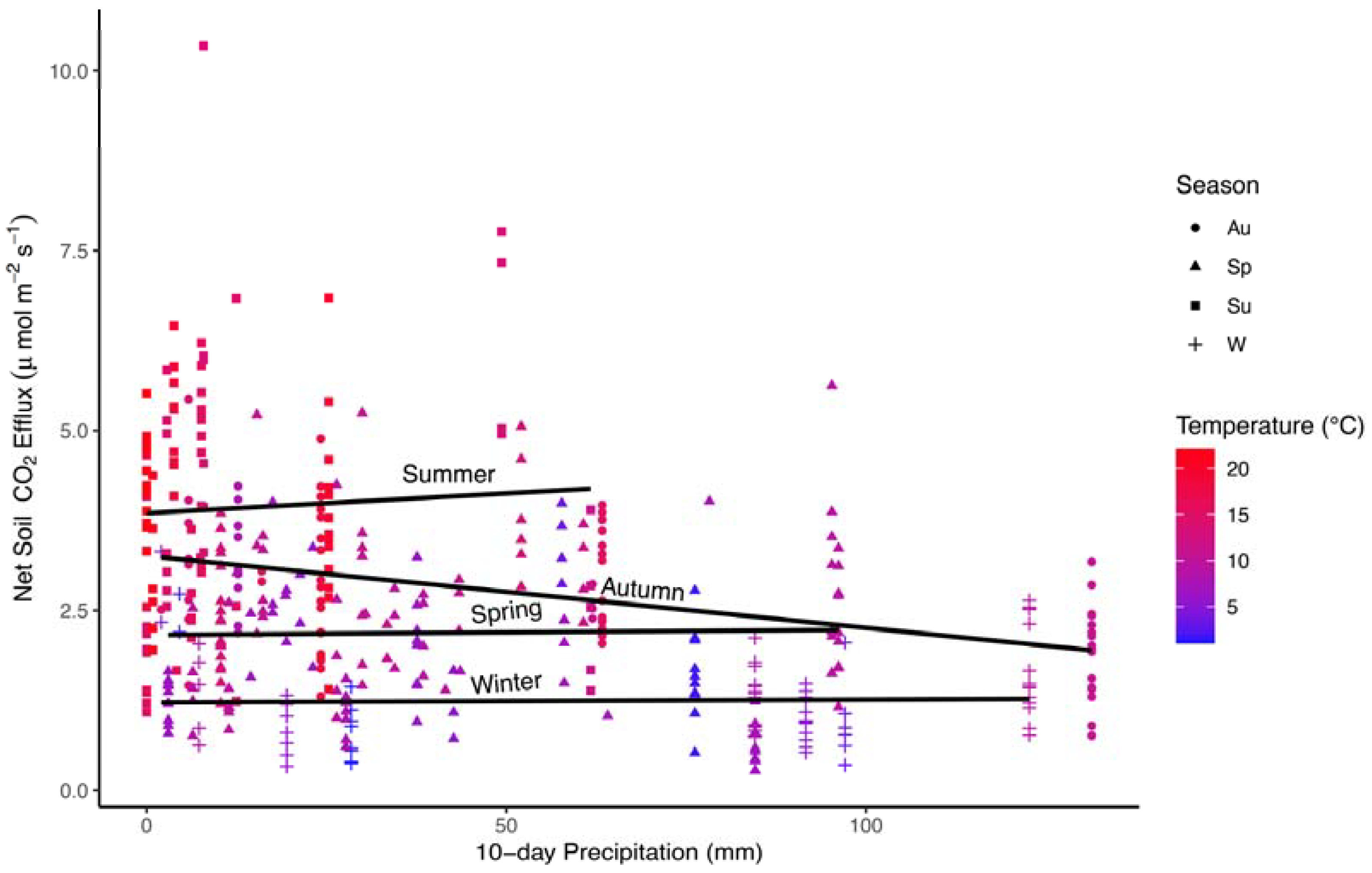
The interaction relationship was particularly complex in autumn, which is typified by droughty conditions with warm temperatures early in the season, and colder wet conditions late in the season. A negative relationship between 10-day precipitation and Fs was apparent in autumn, but inseparable from positive relationships with air temperature on Fs, and differences between seasons in Fs mirrored differences in precipitation and temperature (Figure 3).
Variation in stand type was surprisingly non-significant (Table 1), suggesting that overstory canopy type is not a strong predictor of Fs values in this system. A comparison of average values among stand types through the seasons shows strikingly similar values (Table 2). Average values were 2.43 (95% CI: 2.23–2.63) for conifer stands, 2.74 (95% CI: 2.38–3.10) for mixed conifer and hardwood stands, and 2.56 (95% CI: 2.33–2.80) for hardwood stands.
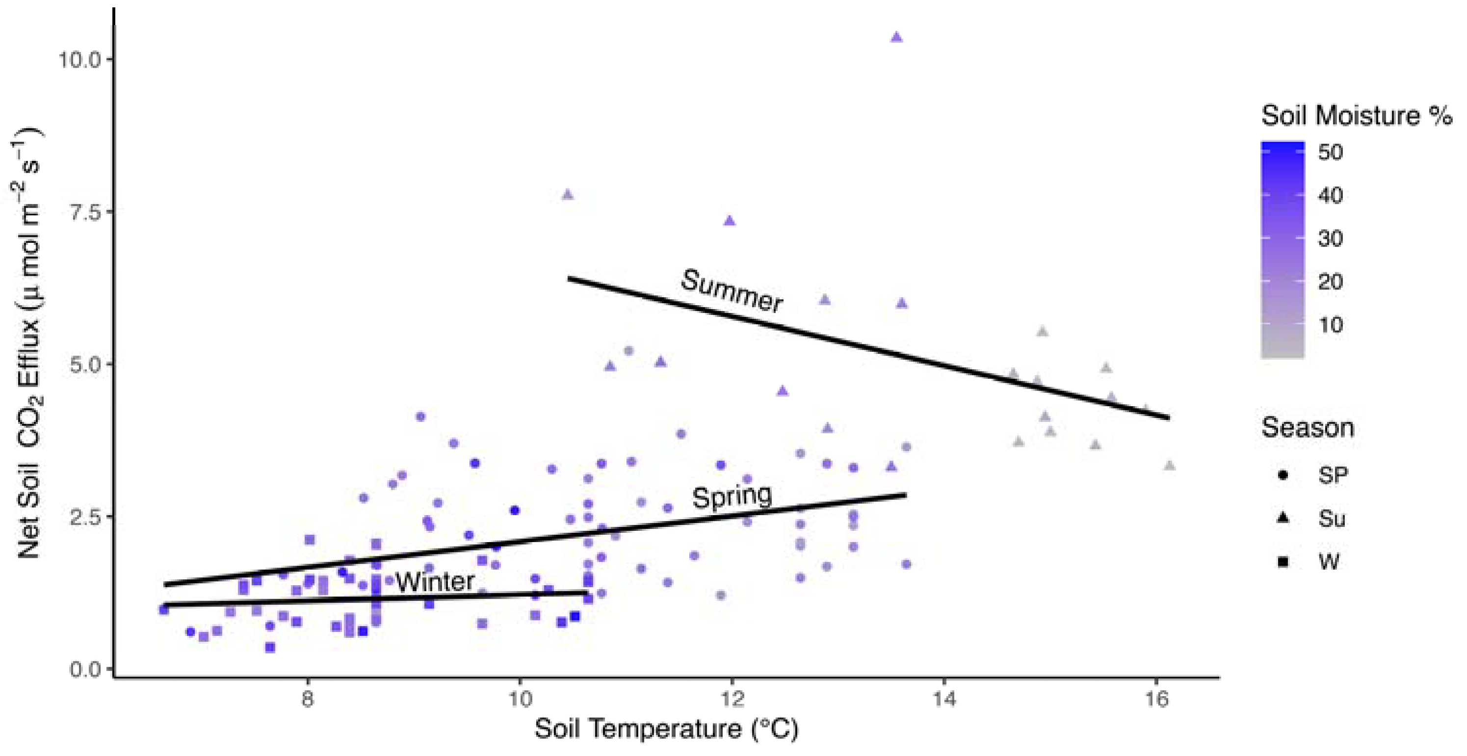
In the model developed for the subset of data where soil moisture and soil temperature data were also available, soil moisture, season, and season by soil temperature interactions were significant factors (Table 3; marginal R2 = 0.582, conditional R2 = 0.797). Soil moisture was a relatively strong negative effect (Fs declined with increasing soil moisture; Figure 4). Soil moisture increases from ~15% in summer (high Fs) to 30% in spring, and >30% in winter were associated with declining Fs. The interaction between soil temperature and season was due to a negative relationship between soil temperature and Fs in the summer (Figure 5). There were no significant interactions between soil moisture and season, but a strong negative correlation between soil temperature and soil moisture (r = −0.957) may have masked this interaction where declines in soil temperature from 16 °C (soil moisture from <10%) to 10 °C (soil moisture >20%) were associated with higher Fs. In the random effects, year accounted for 35.4% of the total variance while plot accounted for only 9.6% (Table S2).
Interactions with season and temperature may have also been reflected in seasonal calculations of Q10. The positive relationship between soil temperature and soil respiration yielded a maximum estimated Q10 value of 3.51 in spring measurements, and a minimum of 1.85 in winter measurements. A negative relationship between Fs and soil temperature, due to droughty conditions when the highest soil temperatures were recorded, resulted in a Q10 of only 0.46 for summer. Thus, while summer Fs values are higher than other seasons, very high soil temperatures may be associated with a decrease in Fs by a factor of 0.46 for every additional 10 °C increase in temperature.
4. Discussion
Over a decade of measurements, we found a clear and consistent seasonal pattern in mean values, where Fs was higher in the summer months and early autumn (Figure 1), and lower in other seasons. While this pattern should not be surprising given the expected abiotic controls over Fs (respiration often increases with temperature and moisture) [40,41], abiotic controls over Fs are not always so clear [42]. Other studies within productive forests of the Pacific Northwest have quantified seasonal trends and provide excellent comparisons with our work [43], even though we know of no similar studies in the lowland Puget Trough biological province. One of the earliest studies of CO2 evolution from forests soils in northwestern ecosystems [44] found evidence of clear seasonality and limited temperature dependence of soil respiration in P. menziezii and A. rubra-dominated forests at about 210 m elevation in Washington State. Similarly, a study along elevation gradients in Olympic National Park found clear predictability of Fs based on soil temperature, and length of growing season, while relationships with soil moisture were more elusive [45]. Other studies from northwestern US [46] have demonstrated seasonality in belowground CO2 flux which could drive higher soil respiration. In other long-term temperate forest studies, inclusion of season or day of year significantly improves models of soil CO2 efflux, reflective of a distinct seasonality in soil respiration [47]. Seasonal variation may be driven by relationships with temperature, but variation in heterotrophic vs. autotrophic respiration responses to temperature and soil moisture can also lead to complex outcomes [48]. For example, tree-root respiration is likely to increase with temperature, but may also increase with belowground activity that occurs outside the aboveground growing season. Here, we were not able to untangle autotrophic and heterotrophic sources, but we were able to document long-term trends in an important C-flux.
We note that while climate patterns in the Pacific Northwest (and other temperate forest biomes) currently conform to standard four-season patterns, climate change may result in more extensive summer droughts, or shorter winters, and hence the utility of a seasonal analysis is dependent on observed climate and weather patterns. Examination of Fs at broader spatial scales and longer time frames will obviously improve generalizable conclusions about spatial and temporal patterns, and will represent an important future research direction. New techniques will necessarily rely on larger data sets such as the one used here for ground-truthing. For example, remote sensing applications are currently under development that may be able to estimate soil respiration based on correlations between soil respiration and soil surface temperature [49,50], and studies such as ours can help parameterize such models more-realistically. Regardless, our data suggest clear seasonality, predictable across more than a decade of measurement, and some potentially important patterns with temperature that may be season and moisture dependent. Our data agree well with the results in global analyses showing clear seasonality in soil respiration in temperate forests, and especially analyses that parse ecosystems with dramatic dry seasons [5,8]. In the long run, such findings will need to be evaluated across changing climate and ecosystem conditions.
While soil respiration (especially heterotrophic Fs) is known to generally increase with temperature and is often quantified using a Q10 relationship [1,39], the exact nature of the relationship is not often understood in individual ecosystems due to the nuances of ecological interactions particular to a given ecosystem [48,51]. A study evaluating Fs across elevation gradients in the Olympic Mountains [45] found ranges in calculated Q10 between 1.6 and 4.9, consistent with our measurements in the present study (1.85–3.51). The mean Q10 calculated in the study (2.9) was also similar to the mean of winter and spring Q10 values from data presented here (2.7). However, we also observed data in which a negative relationship with temperature existed in the summer season and Q10 was below 1.0 (0.46). Our sampling for these values took place during a record drought in 2015 [52], and, while the results were not obvious in our data, excluding the 2015 data resulted in an over-all estimated Q10 of 2.5, close to the median value for Q10 from a broad review of C flux across terrestrial and wetland ecosystems (Q10 = 2.4) [7]. No evidence of Q10 values below 1.0 were reported in average values for the Olympic mountains study [45], but the authors of that study found weak moisture effects and it’s possible that moisture was not limiting in these mountainous sites over the limited one-year time frame of the study. Our estimates of Q10 are also well within the range expected for temperate forests based on global reviews of Q10 values [1].
We hypothesized that dominant tree canopy type would significantly predict patterns and rates of Fs. Our analysis of Fs did not indicate any evidence of distinct patterning among forests dominated by either coniferous, deciduous, or mixed tree species (Table 2). While plot identity accounted for a large amount of random effect variance measures, plot overstory was not a significant predictor of Fs. This result was somewhat surprising based on earlier work where Fs was found to vary positively with tree species diversity [30]. Our findings, however, are not inconsistent with this earlier work in that higher values of Fs were found in mixed stands (Table 2), even though stand type was not a significant factor in models. Additionally, over longer time periods, it is possible that diversity effects present in a single year may become more diffuse. Overall, these data suggest that even if significant differences in stand type can occur, long-term sampling produces similar estimates of CO2 flux from soils in adjacent stand types. We note that, although dominant stand type varied from coniferous to deciduous and mixed tree species dominance, all stands were similar in age and soil type [35].
5. Conclusions
Our long-term (~15-year) dataset suggests annual Fs fluxes (through CO2) of ~9.5 Mg C ha−1 year−1, with 1.16 Mg C ha−1 in winter, 2.04 Mg C ha−1 in spring, 3.84 Mg C ha−1 in summer, and 2.45 Mg C ha−1 in autumn seasons. Since more than 50% of Fs may represent heterotrophic respiration of CO2 [6,28,42], this suggests that this highly productive system may have annual heterotrophic soil respiration rates as high or higher than 4.75 Mg C ha−1 year−1. Complex interactions with soil moisture and temperature lead to variation in predictability of Fs based on abiotic factors throughout different seasons. Variability in summer and autumn Fs rates are particularly important for understanding changes in annual flux rates of C from soils to atmospheric pools since these seasons contain the highest Fs rates. Quantifying summer season responses to combinations of increasing temperatures and low soil moisture will be particularly critical in this bioregion for detecting changes in Fs in response to future climate change.
Supplementary Materials
The following supporting information can be downloaded at: https://www.mdpi.com/article/10.3390/f15010161/s1, Table S1: Model parameter and random effects model output for average plot Fs (μmol C m−2 s−1) LMER mixed effects model including season, stand type, 10-day precipitation and air-temperature as fixed effects.; Table S2: Model parameter and random effects model output for a mixed-effects LMER model for a subset of Fs (μmol C m−2 s−1) data where soil moisture and air-temperature were included as fixed effects in addition to season.
Author Contributions
Conceptualization, D.G.F.; methodology, D.G.F.; formal analysis, D.G.F.; resources, D.G.F.; data curation, D.G.F., C.E.C., R.A.M. and L.O.M.; fieldwork, R.A.M., C.E.C., D.G.F., L.O.M. and Z.R.C.; writing—original draft preparation, D.G.F.; writing—review and editing, D.G.F., C.E.C. and Z.R.C.; visualization, D.G.F.; supervision, D.G.F.; project administration, D.G.F.; funding acquisition, D.G.F. All authors have read and agreed to the published version of the manuscript.
Funding
This work was supported by The Evergreen State College Sabbatical Support to Dylan Fischer, The Evergreen State College Foundation, Evergreen Sponsored Research, The Evergreen Summer Undergraduate Research Fellowship, and The Evergreen Fund for Innovation, and Microsoft Corporation.
Data Availability Statement
Data are available through the Open Science Framework website: https://osf.io/2xyk9, accessed on 11 January 2023; DOI 10.17605/OSF.IO/2XYK9.
Acknowledgments
This work would not have been possible without the dedication and hard work of Justin Kirsch, Alex Kazakova, Thomas Otto, Erik Rook, Todd McCaslin, Andy Berger, Shayna Rossiter, Mathew Brousil, Tristan Weiss, Deja Malone, Margaret Pryor, Ruth Mares, Gabe Chavez, Bret McNamara, Choddington Kumal, Brandy Ranger, Leighton Olive, Jamie Bown, Vanessa Ryder, Alice Fischer, Rob Cole, Jora Rehm-Lorber, Kyle Galloway, Pat Babbin, Josh Brann, Jordan Erickson, Don Loft, Katherine Halstead, Christopher Anthony, Casey Broderick, Emily Anderson and Lindsey Wright. Alison Styring and Paul Przybylowicz contributed to initial plot design (Styring) and establishment (Przybylowicz). Carri LeRoy entertained multiple conversations at intermediate stages of the work. We also thank staff and students at the Evergreen Science Support Center and the Evergreen Science Instructional Technicians for help with equipment. Finally, we thank two anonymous reviewers and editors at Forests for comments and suggestions.
Conflicts of Interest
The authors declare no conflicts of interest.
References
- Kirschbaum, M.U.F. The Temperature Dependence of Soil Organic Matter Decomposition, and the Effect of Global Warming on Soil Organic C Storage. Soil Biol. Biochem. 1995, 27, 753–760. [Google Scholar] [CrossRef]
- Luyssaert, S.; Schulze, E.-D.; Börner, A.; Knohl, A.; Hessenmöller, D.; Law, B.E.; Ciais, P.; Grace, J. Old-Growth Forests as Global Carbon Sinks. Nature 2008, 455, 213–215. [Google Scholar] [CrossRef] [PubMed]
- Ciais, P.; Sabine, C.; Bala, G.; Bopp, L.; Brovkin, V.; Canadell, J.; Chhabra, A.; DeFries, R.; Galloway, J.; Heimann, M.; et al. The Physical Science Basis. Contribution of Working Group I to the Fifth Assessment Report of the Intergovernmental Panel on Climate Change; IPCC Climate: Geneva, Switzerland, 2013. [Google Scholar]
- Oertel, C.; Matschullat, J.; Zurba, K.; Zimmermann, F.; Erasmi, S. Greenhouse Gas Emissions from Soils—A Review. Geochemistry 2016, 76, 327–352. [Google Scholar] [CrossRef]
- Dixon, R.K.; Solomon, A.M.; Brown, S.; Houghton, R.A.; Trexier, M.C.; Wisniewski, J. Carbon Pools and Flux of Global Forest Ecosystems. Science 1994, 263, 185–190. [Google Scholar] [CrossRef] [PubMed]
- Litton, C.M.; Raich, J.W.; Ryan, M.G. Carbon Allocation in Forest Ecosystems. Glob. Chang. Biol. 2007, 13, 2089–2109. [Google Scholar] [CrossRef]
- Raich, J.W.; Schlesinger, W.H. The Global Carbon Dioxide Flux in Soil Respiration and Its Relationship to Vegetation and Climate. Tellus B 1992, 44, 81–99. [Google Scholar] [CrossRef]
- Raich, J.W.; Potter, C.S. Global Patterns of Carbon Dioxide Emissions from Soils. Glob. Biogeochem. Cycles 1995, 9, 23–36. [Google Scholar] [CrossRef]
- Jobbágy, E.G.; Jackson, R.B. The Vertical Distribution of Soil Organic Carbon and Its Relation to Climate and Vegetation. Ecol. Appl. 2000, 10, 423–436. [Google Scholar] [CrossRef]
- Raich, J.W. Temporal Variability of Soil Respiration in Experimental Tree Plantations in Lowland Costa Rica. Forests 2017, 8, 40. [Google Scholar] [CrossRef]
- Phillips, C.L.; Bond-Lamberty, B.; Desai, A.R.; Lavoie, M.; Risk, D.; Tang, J.; Todd-Brown, K.; Vargas, R. The Value of Soil Respiration Measurements for Interpreting and Modeling Terrestrial Carbon Cycling. Plant Soil 2017, 413, 1–25. [Google Scholar] [CrossRef]
- Kern, J.S. Spatial Patterns of Soil Organic Carbon in the Contiguous United States. Soil Sci. Soc. Am. J. 1994, 58, 439–455. [Google Scholar] [CrossRef]
- Turner, D.P.; Koerper, G.J.; Harmon, M.E.; Lee, J.J. A Carbon Budget for Forests of the Conterminous United States. Ecol. Appl. 1995, 5, 421–436. [Google Scholar] [CrossRef]
- Singh, J.S.; Gupta, S.R. Plant Decomposition and Soil Respiration in Terrestrial Ecosystems. Bot. Rev. 1977, 43, 449–528. [Google Scholar] [CrossRef]
- Schlentner, R.E.; Cleve, K.V. Relationships between CO2 Evolution from Soil, Substrate Temperature, and Substrate Moisture in Four Mature Forest Types in Interior Alaska. Can. J. For. Res. 1985, 15, 97–106. [Google Scholar] [CrossRef]
- Carlyle, J.C.; Than, U.B. Abiotic Controls of Soil Respiration Beneath an Eighteen-Year-Old Pinus Radiata Stand in South-Eastern Australia. J. Ecol. 1988, 76, 654–662. [Google Scholar] [CrossRef]
- Bond-Lamberty, B.; Thomson, A. Temperature-Associated Increases in the Global Soil Respiration Record. Nature 2010, 464, 579–582. [Google Scholar] [CrossRef]
- Raich, J.W.; Lambers, H.; Oliver, D.J. 10.16—Respiration in Terrestrial Ecosystems. In Treatise on Geochemistry, 2nd ed.; Holland, H.D., Turekian, K.K., Eds.; Elsevier: Oxford, UK, 2014; pp. 613–649. ISBN 978-0-08-098300-4. [Google Scholar]
- Cisneros-Dozal, L.M.; Trumbore, S.; Hanson, P.J. Partitioning Sources of Soil-Respired CO2 and Their Seasonal Variation Using a Unique Radiocarbon Tracer. Glob. Chang. Biol. 2005, 12, 194–204. [Google Scholar] [CrossRef]
- Campbell, J.L.; Sun, O.J.; Law, B.E. Supply-Side Controls on Soil Respiration among Oregon Forests. Glob. Chang. Biol. 2004, 10, 1857–1869. [Google Scholar] [CrossRef]
- Campbell, J.L.; Law, B.E. Forest Soil Respiration across Three Climatically Distinct Chronosequences in Oregon. Biogeochemistry 2005, 73, 109–125. [Google Scholar] [CrossRef]
- Taylor, A.J.; Lai, C.-T.; Hopkins, F.M.; Wharton, S.; Bible, K.; Xu, X.; Phillips, C.; Bush, S.; Ehleringer, J.R. Radiocarbon-Based Partitioning of Soil Respiration in an Old-Growth Coniferous Forest. Ecosystems 2015, 18, 459–470. [Google Scholar] [CrossRef]
- Waring, R.H.; Franklin, J.F. Evergreen Coniferous Forests of the Pacific Northwest. Science 1979, 204, 1380–1386. [Google Scholar] [CrossRef] [PubMed]
- Lundegårdh, H. Carbon Dioxide Evolution of Soil and Crop Growth. Soil Sci. 1927, 23, 417. [Google Scholar] [CrossRef]
- Lieth, H.; Ouellette, R. Studies on the Vegetation of the Gaspé Peninsula: Ii. the Soil Respiration of Some Plant Communities. Can. J. Bot. 1962, 40, 127–140. [Google Scholar] [CrossRef]
- Ellis, R.C. The Seasonal Pattern of Nitrogen and Carbon Mineralization in Forest and Pasture Soils in Southern Ontario. Can. J. Soil. Sci. 1974, 54, 15–28. [Google Scholar] [CrossRef]
- Schlesinger, W.H. Carbon Balance in Terrestrial Detritus. Annu. Rev. Ecol. Syst. 1977, 8, 51–81. [Google Scholar] [CrossRef]
- Fischer, D.G.; Hart, S.C.; LeRoy, C.J.; Whitham, T.G. Variation in Below-Ground Carbon Fluxes along a Populus Hybridization Gradient. New Phytol. 2007, 176, 415–425. [Google Scholar] [CrossRef] [PubMed]
- Lojewski, N.R.; Fischer, D.G.; Bailey, J.K.; Schweitzer, J.A.; Whitham, T.G.; Hart, S.C. Genetic Basis of Aboveground Productivity in Two Native Populus Species and Their Hybrids. Tree Physiol. 2009, 29, 1133–1142. [Google Scholar] [CrossRef]
- Kirsch, J.L.; Fischer, D.G.; Kazakova, A.N.; Biswas, A.; Kelm, R.E.; Carlson, D.W.; LeRoy, C.J. Diversity-Carbon Flux Relationships in a Northwest Forest. Diversity 2012, 4, 33–58. [Google Scholar] [CrossRef]
- LeRoy, C.J.; Fischer, D.G. Do Genetically-Specific Tree Canopy Environments Feed Back to Affect Genetically Specific Leaf Decomposition Rates? Plant Soil 2019, 437, 1–10. [Google Scholar] [CrossRef]
- Metcalfe, D.B.; Fisher, R.A.; Wardle, D.A. Plant Communities as Drivers of Soil Respiration: Pathways, Mechanisms, and Significance for Global Change. Biogeosciences 2011, 8, 2047–2061. [Google Scholar] [CrossRef]
- Chen, X.; Chen, H.Y.H. Plant Diversity Loss Reduces Soil Respiration across Terrestrial Ecosystems. Glob. Chang. Biol. 2019, 25, 1482–1492. [Google Scholar] [CrossRef] [PubMed]
- Luan, J.; Liu, S.; Wang, J.; Chang, S.X.; Liu, X.; Lu, H.; Wang, Y. Tree Species Diversity Promotes Soil Carbon Stability by Depressing the Temperature Sensitivity of Soil Respiration in Temperate Forests. Sci. Total Environ. 2018, 645, 623–629. [Google Scholar] [CrossRef] [PubMed]
- Rex, I.; Fischer, D.G.; Bartlett, R. A Decade of Understory Community Dynamics and Stability in a Mature Second-Growth Forest in Western Washington. Northwest Sci. 2023, 96, 164–183. [Google Scholar] [CrossRef]
- Cueva, A.; Bullock, S.H.; López-Reyes, E.; Vargas, R. Potential Bias of Daily Soil CO2 Efflux Estimates Due to Sampling Time. Sci. Rep. 2017, 7, 11925. [Google Scholar] [CrossRef] [PubMed]
- Bates, D.; Mächler, M.; Bolker, B.; Walker, S. Fitting Linear Mixed-Effects Models Using Lme4. J. Stat. Softw. 2015, 67, 1–48. [Google Scholar] [CrossRef]
- R Core Team. R: A Language and Environment for Statistical Computing; R Foundation for Statistical Computing: Vienna, Austria, 2023. [Google Scholar]
- Van’t Hoff, J.H. Lectures on Theoretical and Physical Chemistry. In Part I. Chemical Dynamics; Lehfeld, R.A., Translator; Edward Arnold: London, UK, 1898. [Google Scholar]
- Orchard, V.A.; Cook, F.J. Relationship between Soil Respiration and Soil Moisture. Soil Biol. Biochem. 1983, 15, 447–453. [Google Scholar] [CrossRef]
- Kirschbaum, M.U.F. The Temperature Dependence of Organic-Matter Decomposition—Still a Topic of Debate. Soil Biol. Biochem. 2006, 38, 2510–2518. [Google Scholar] [CrossRef]
- Giardina, C.P.; Ryan, M.G. Evidence That Decomposition Rates of Organic Carbon in Mineral Soil Do Not Vary with Temperature. Nature 2000, 404, 858–861. [Google Scholar] [CrossRef]
- Drewitt, G.B.; Black, T.A.; Nesic, Z.; Humphreys, E.R.; Jork, E.M.; Swanson, R.; Ethier, G.J.; Griffis, T.; Morgenstern, K. Measuring Forest Floor CO2 Fluxes in a Douglas-Fir Forest. Agric. For. Meteorol. 2002, 110, 299–317. [Google Scholar] [CrossRef]
- Vogt, K.A.; Edmonds, R.L.; Antos, G.C.; Vogt, D.J. Relationships between CO2 Evolution, ATP Concentrations and Decomposition in Four Forest Ecosystems in Western Washington. Oikos 1980, 35, 72–79. [Google Scholar] [CrossRef]
- Kane, E.S.; Pregitzer, K.S.; Burton, A.J. Soil Respiration along Environmental Gradients in Olympic National Park. Ecosystems 2003, 6, 326–335. [Google Scholar] [CrossRef]
- Vogt, K.A.; Grier, C.C.; Meier, C.E.; Edmonds, R.L. Mycorrhizal Role in Net Primary Priduction and Nutrient Cytcling in Abies Amabilis Ecosystems in Western Washington. Ecology 1982, 63, 370–380. [Google Scholar] [CrossRef]
- Acosta, M.; Darenova, E.; Krupková, L.; Pavelka, M. Seasonal and Inter-Annual Variability of Soil CO2 Efflux in a Norway Spruce Forest over an Eight-Year Study. Agric. For. Meteorol. 2018, 256–257, 93–103. [Google Scholar] [CrossRef]
- Ryan, M.G.; Law, B.E. Interpreting, Measuring, and Modeling Soil Respiration. Biogeochemistry 2005, 73, 3–27. [Google Scholar] [CrossRef]
- Huang, N.; Gu, L.; Black, T.A.; Wang, L.; Niu, Z. Remote Sensing-Based Estimation of Annual Soil Respiration at Two Contrasting Forest Sites. J. Geophys. Res. Biogeosci. 2015, 120, 2306–2325. [Google Scholar] [CrossRef]
- Crabbe, R.A.; Janouš, D.; Dařenová, E.; Pavelka, M. Exploring the Potential of LANDSAT-8 for Estimation of Forest Soil CO2 Efflux. Int. J. Appl. Earth Obs. Geoinf. 2019, 77, 42–52. [Google Scholar] [CrossRef]
- Johnston, A.S.A.; Sibly, R.M. The Influence of Soil Communities on the Temperature Sensitivity of Soil Respiration. Nat. Ecol. Evol. 2018, 2, 1597–1602. [Google Scholar] [CrossRef]
- Marlier, M.E.; Xiao, M.; Engel, R.; Livneh, B.; Abatzoglou, J.T.; Lettenmaier, D.P. The 2015 Drought in Washington State: A Harbinger of Things to Come? Environ. Res. Lett. 2017, 12, 114008. [Google Scholar] [CrossRef]
Figure 1.
Violin plots of soil CO2 efflux values (μmol CO2 m−2 s−1) by month throughout sampling period (2008–2023). Colors represent distinct seasons: winter (W; purple), spring (Sp; green), summer (Su; blue), and autumn (Au; orange). Black boxes represent the mean for each group, while colored shapes and points represent the data distribution and outlier values.

Figure 2.
Scatterplot of average monthly Fs values (μmol CO2 m−2 s−1) by air temperature (°C) in all four seasons. Lines are fit to data independently within each season. Colors represent summative precipitation values (mm) for 10 days prior to measurements. Shapes represent different seasons for autumn (Au; circles), spring (Sp; triangles), summer (Su; squares), and winter (W; crosses).

Figure 3.
Scatterplot of average monthly Fs values (μmol C m−2 s−1) by precipitation (mm) in all four seasons. Lines are fit to data independently within each season. Colors represent average temperature (°C). Shapes represent different seasons for autumn (Au; circles), spring (Sp; triangles), summer (Su; squares), and winter (W; crosses).

Figure 4.
Scatterplot of average monthly Fs values (μmol CO2 m−2 s−1) by soil moisture (%) for a subset of data in in all three seasons where data were available. Lines are fit to data independently within each season. Colors represent soil temperature (°C). Shapes reflect seasons: spring (Sp; circles), summer (Su; triangles), and winter (W; squares).
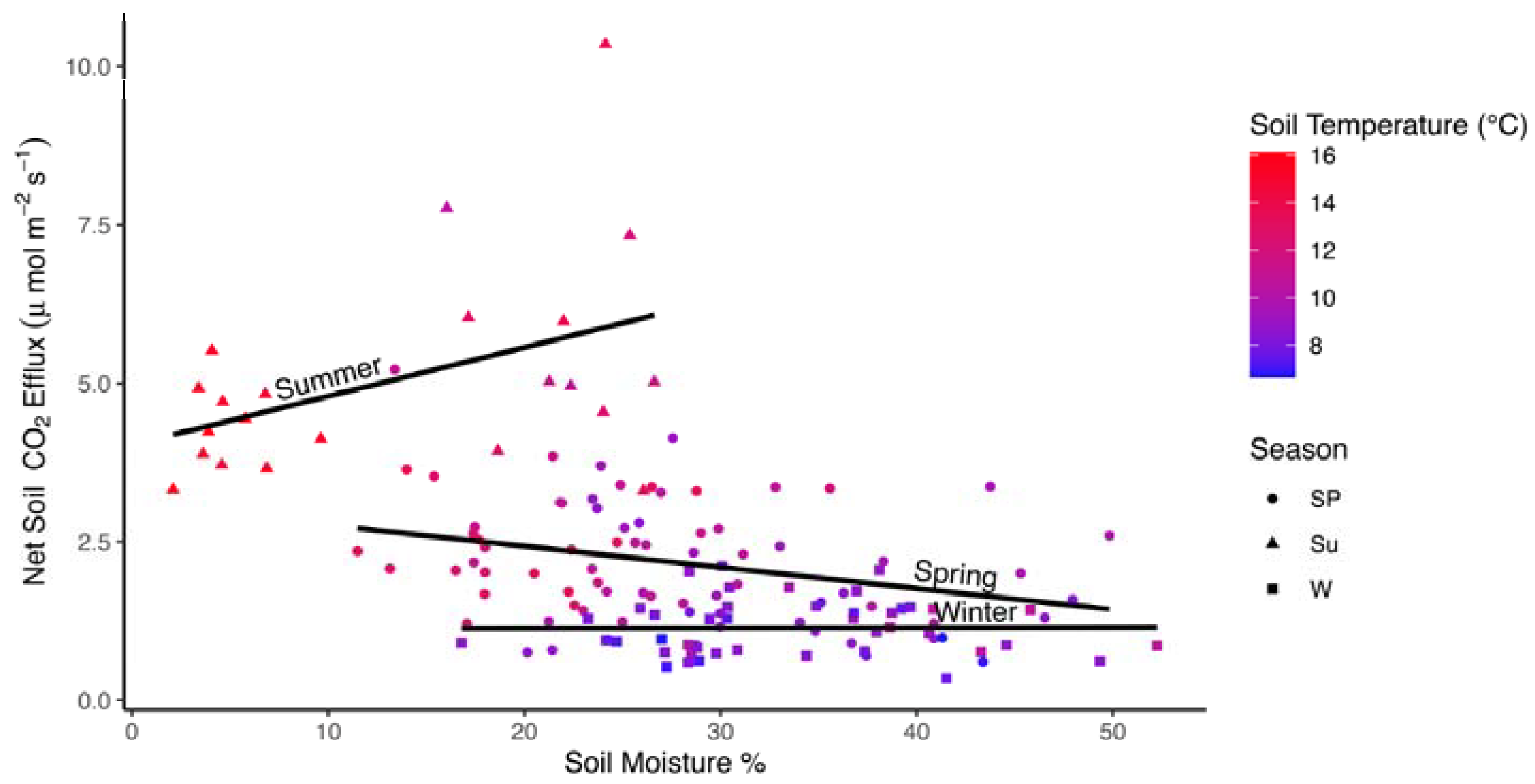
Figure 5.
Scatterplot of average monthly Fs values (μmol CO2 m−2 s−1) by soil temperature (°C) for a subset of data in in all three seasons where data were available. Lines are fit to data independently within each season. Colors represent soil moisture (%). Shapes reflect seasons: spring (Sp; circles), summer (Su; triangles), and winter (W; squares).


Table 1.
Type III analysis of variance table for average plot Fs (μmol C m−2 s−1) values (significant p-values shown in bold).
Table 1.
Type III analysis of variance table for average plot Fs (μmol C m−2 s−1) values (significant p-values shown in bold).
| Factor | SS | MS | dfnum/dfden | F | p |
|---|---|---|---|---|---|
| Season | 9.40 | 3.14 | 3/36.08 | 4.47 | 0.009 |
| Stand Type | 1.75 | 0.87 | 2/22.88 | 1.25 | 0.306 |
| Precipitation (10-day mm) | 0.62 | 0.620 | 1/63.28 | 0.88 | 0.351 |
| Temperature (°C) | 5.92 | 5.92 | 1/62.19 | 8.44 | 0.005 |
| Season: Stand Type | 8.89 | 1.48 | 6/355.86 | 2.11 | 0.051 |
| Precipitation: Temperature | 0.48 | 0.48 | 1/69.12 | 0.68 | 0.412 |
| Season: Precipitation | 17.00 | 5.67 | 3/102.31 | 8.08 | <0.001 |
| Season: Temperature | 10.17 | 3.39 | 3/71.65 | 4.83 | 0.004 |
| Season: Precipitation: Temperature | 19.11 | 6.37 | 3/105.84 | 9.08 | <0.001 |
Table 2.
Average seasonal values for Fs (μmol C m−2 s−1) along with 95% confidence intervals in deciduous, coniferous, and mixed stand types.
Table 2.
Average seasonal values for Fs (μmol C m−2 s−1) along with 95% confidence intervals in deciduous, coniferous, and mixed stand types.
| Season | Canopy Type | n | Average | SE | CV | ±95% CI |
|---|---|---|---|---|---|---|
| Spring | Conifer | 74 | 2.16 | 0.12 | 49.61 | 0.2 |
| Mixed Conifer and Hardwood | 37 | 2.28 | 0.21 | 56.15 | 0.4 | |
| Hardwood | 49 | 2.17 | 0.13 | 41.45 | 0.3 | |
| Summer | Conifer | 49 | 3.57 | 0.21 | 40.77 | 0.4 |
| Mixed Conifer and Hardwood | 18 | 4.76 | 0.49 | 43.41 | 1.0 | |
| Hardwood | 29 | 3.99 | 0.30 | 39.94 | 0.6 | |
| Autumn | Conifer | 35 | 2.49 | 0.16 | 38.83 | 0.3 |
| Mixed Conifer and Hardwood | 20 | 3.07 | 0.21 | 30.85 | 0.4 | |
| Hardwood | 27 | 2.77 | 0.15 | 28.29 | 0.3 | |
| Winter | Conifer | 29 | 1.13 | 0.13 | 61.52 | 0.3 |
| Mixed Conifer and Hardwood | 17 | 1.23 | 0.15 | 51.69 | 0.3 | |
| Hardwood | 24 | 1.40 | 0.12 | 40.50 | 0.2 |
Table 3.
Type III analysis of variance table for average plot Fs values (μmol C m−2 s−1) for a data subset that included soil moisture and temperature in winter, spring, and summer seasons (significant p-values shown in bold).
Table 3.
Type III analysis of variance table for average plot Fs values (μmol C m−2 s−1) for a data subset that included soil moisture and temperature in winter, spring, and summer seasons (significant p-values shown in bold).
| Factor | SS | MS | dfnum/dfden | F | p |
|---|---|---|---|---|---|
| Soil Moisture (10 cm depth) | 2.20 | 2.20 | 1/113.95 | 4.13 | 0.044 |
| Soil Temperature (°C) | 0.70 | 0.70 | 1/113.89 | 1.32 | 0.254 |
| Season | 5.33 | 2.67 | 2/115.9 | 5.00 | 0.008 |
| Soil Moisture: Soil Temperature | 2.04 | 2.04 | 1/114.06 | 3.82 | 0.053 |
| Season: Soil Moisture | 2.02 | 1.01 | 2/117.02 | 1.89 | 0.155 |
| Season: Temperature | 4.34 | 2.17 | 2/116.47 | 4.07 | 0.020 |
| Season: Precipitation: Temperature | 2.08 | 1.04 | 2/117.61 | 1.95 | 0.147 |
Disclaimer/Publisher’s Note: The statements, opinions and data contained in all publications are solely those of the individual author(s) and contributor(s) and not of MDPI and/or the editor(s). MDPI and/or the editor(s) disclaim responsibility for any injury to people or property resulting from any ideas, methods, instructions or products referred to in the content. |
© 2024 by the authors. Licensee MDPI, Basel, Switzerland. This article is an open access article distributed under the terms and conditions of the Creative Commons Attribution (CC BY) license (https://creativecommons.org/licenses/by/4.0/).
Share and Cite
MDPI and ACS Style
Fischer, D.G.; Chamberlain, Z.R.; Cook, C.E.; Martin, R.A.; Mueller, L.O. Long-Term Patterns in Forest Soil CO2 Flux in a Pacific Northwest Temperate Rainforest. Forests 2024, 15, 161. https://doi.org/10.3390/f15010161
AMA Style
Fischer DG, Chamberlain ZR, Cook CE, Martin RA, Mueller LO. Long-Term Patterns in Forest Soil CO2 Flux in a Pacific Northwest Temperate Rainforest. Forests. 2024; 15(1):161. https://doi.org/10.3390/f15010161
Chicago/Turabian StyleFischer, Dylan G., Zoe R. Chamberlain, Claire E. Cook, Randall Adam Martin, and Liam O. Mueller. 2024. "Long-Term Patterns in Forest Soil CO2 Flux in a Pacific Northwest Temperate Rainforest" Forests 15, no. 1: 161. https://doi.org/10.3390/f15010161
Note that from the first issue of 2016, this journal uses article numbers instead of page numbers. See further details here.