Modeling Survival, Yield, Volume Partitioning and Their Response to Thinning for Longleaf Pine Plantations

 , , and
Abstract
:1. Introduction
2. Materials and Methods
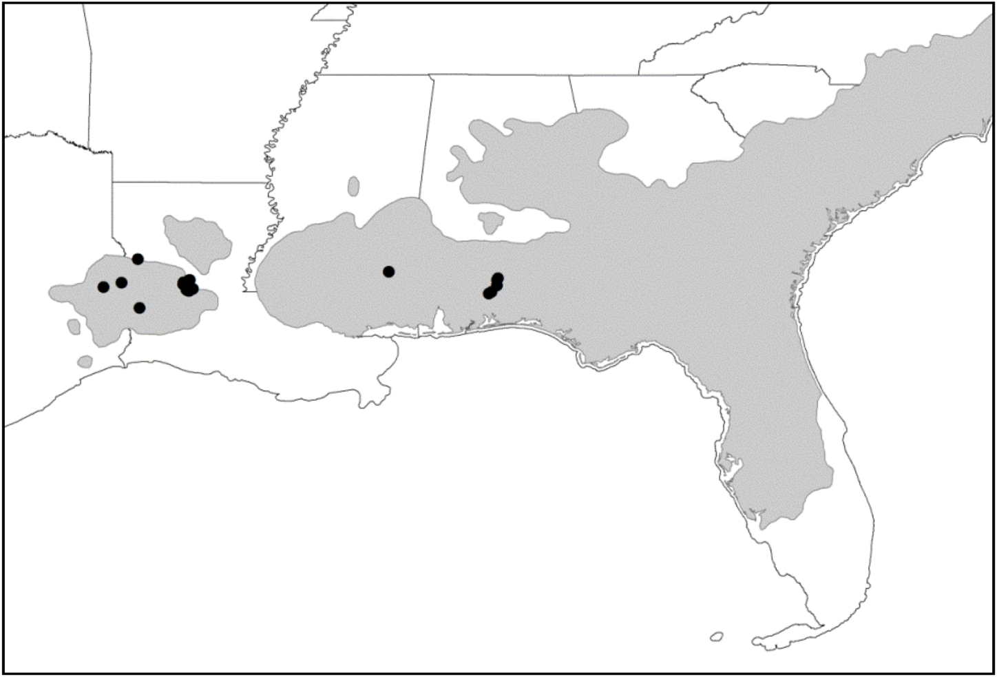
2.1. Data Description


| Variable | Model fitting dataset (237 plots) | Model evaluation dataset (30 plots) | ||||||||
|---|---|---|---|---|---|---|---|---|---|---|
| Mean | SD | Minimum | Maximum | n | Mean | SD | Minimum | Maximum | n | |
| Age | 35.9 | 15.7 | 7.0 | 73.0 | 725 | 36.8 | 16.3 | 7.0 | 73.0 | 140 |
| dbh | 21.6 | 8.3 | 6.8 | 44.1 | 725 | 21.6 | 7.8 | 6.8 | 42.4 | 140 |
| H | 18.6 | 5.3 | 5.3 | 30.1 | 725 | 19.3 | 5.8 | 5.4 | 30.5 | 140 |
| N | 865 | 504 | 99 | 2849 | 725 | 982 | 548 | 198 | 2422 | 140 |
| BA | 27.0 | 11.3 | 6.6 | 62.9 | 725 | 31.5 | 13.1 | 6.8 | 65.9 | 140 |
| Dq | 22.6 | 8.4 | 7.0 | 44.3 | 725 | 22.6 | 8.0 | 7.1 | 42.8 | 140 |
| SDI | 566 | 222 | 129 | 1222 | 725 | 655 | 250 | 144 | 1287 | 140 |
| Hdom | 20.6 | 5.6 | 6.7 | 32.0 | 725 | 21.5 | 6.1 | 6.4 | 32.8 | 140 |
| SI | 25.8 | 1.9 | 19.6 | 30.8 | 173 * | 26.4 | 1.6 | 22.1 | 29.3 | 21 * |
| VOLOB | 274.6 | 141.2 | 46.7 | 688.6 | 725 | 320.7 | 161.4 | 55.0 | 701.3 | 140 |
| Surviving Density Class (ha−1) | Stand Age Class (yrs.) | ||||
|---|---|---|---|---|---|
| 7–20 | 20–40 | 40–60 | 60–73 | Total | |
| 99–500 | 8 | 66 | 105 | 61 | 240 |
| 500–1000 | 51 | 112 | 91 | 17 | 271 |
| 1000–1500 | 69 | 153 | 27 | - | 249 |
| 1500–2000 | 36 | 49 | 2 | - | 87 |
| 2000–2849 | 10 | 8 | - | - | 18 |
| Site Index Class (m) * | |||||
| 19–22 | 4 | 45 | 12 | 4 | 35 |
| 22–25 | 46 | 78 | 46 | 21 | 191 |
| 25–28 | 49 | 217 | 132 | 49 | 447 |
| 28–31 | 75 | 78 | 35 | 4 | 192 |
| Total | 174 | 388 | 225 | 78 | 865 |
2.2. Model Description
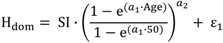
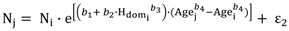
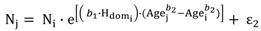
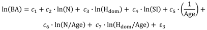
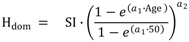
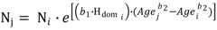
2.2.1. Survival and Yield Models for Unthinned Stands


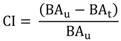
2.2.2. Basal Area Growth Model for Thinned Stands
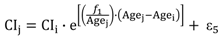
 , corresponds to the annual decline rate of the CI as the stand ages after thinning.
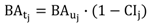
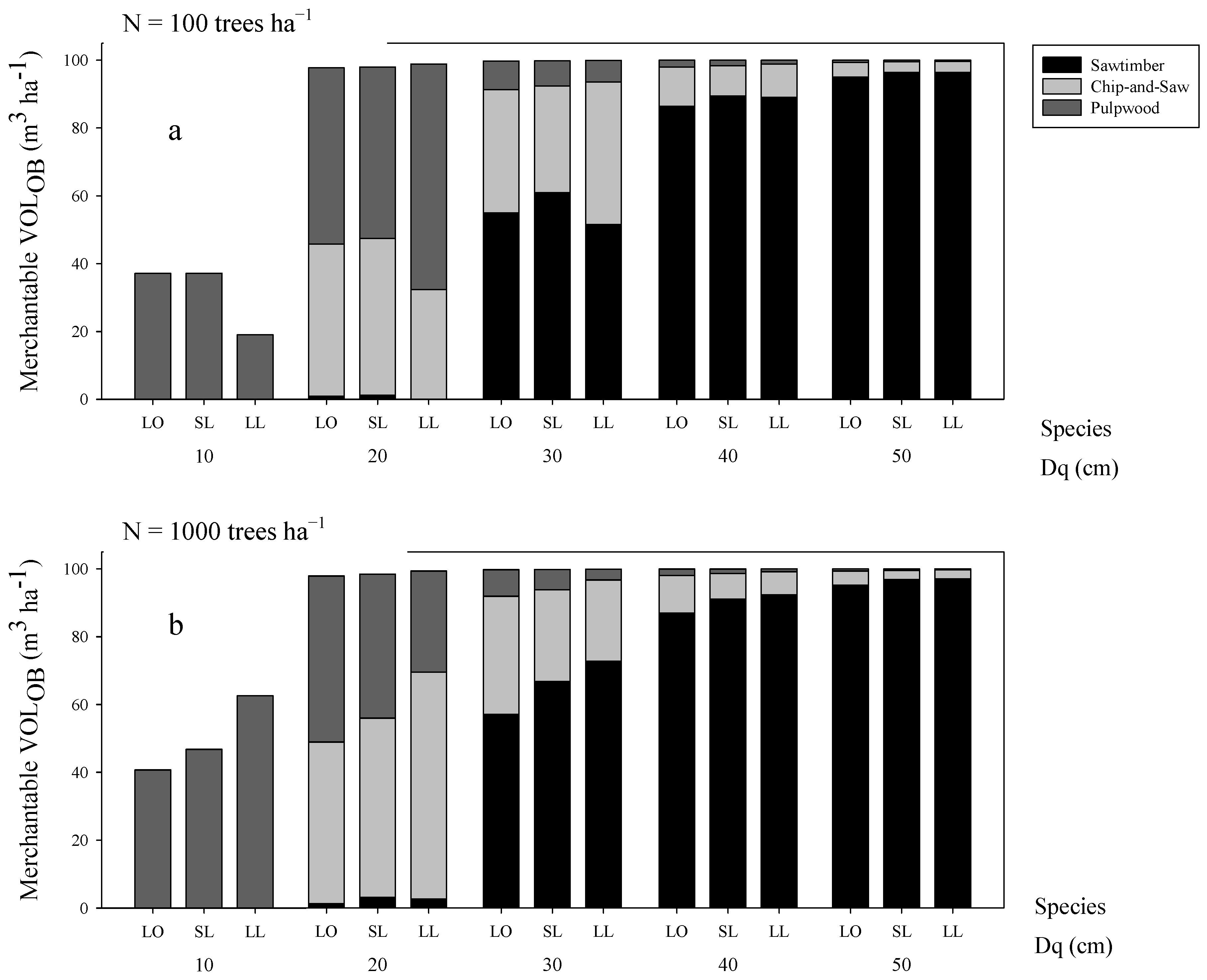
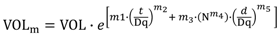
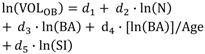
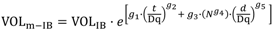
2.2.3. Merchantable Volume
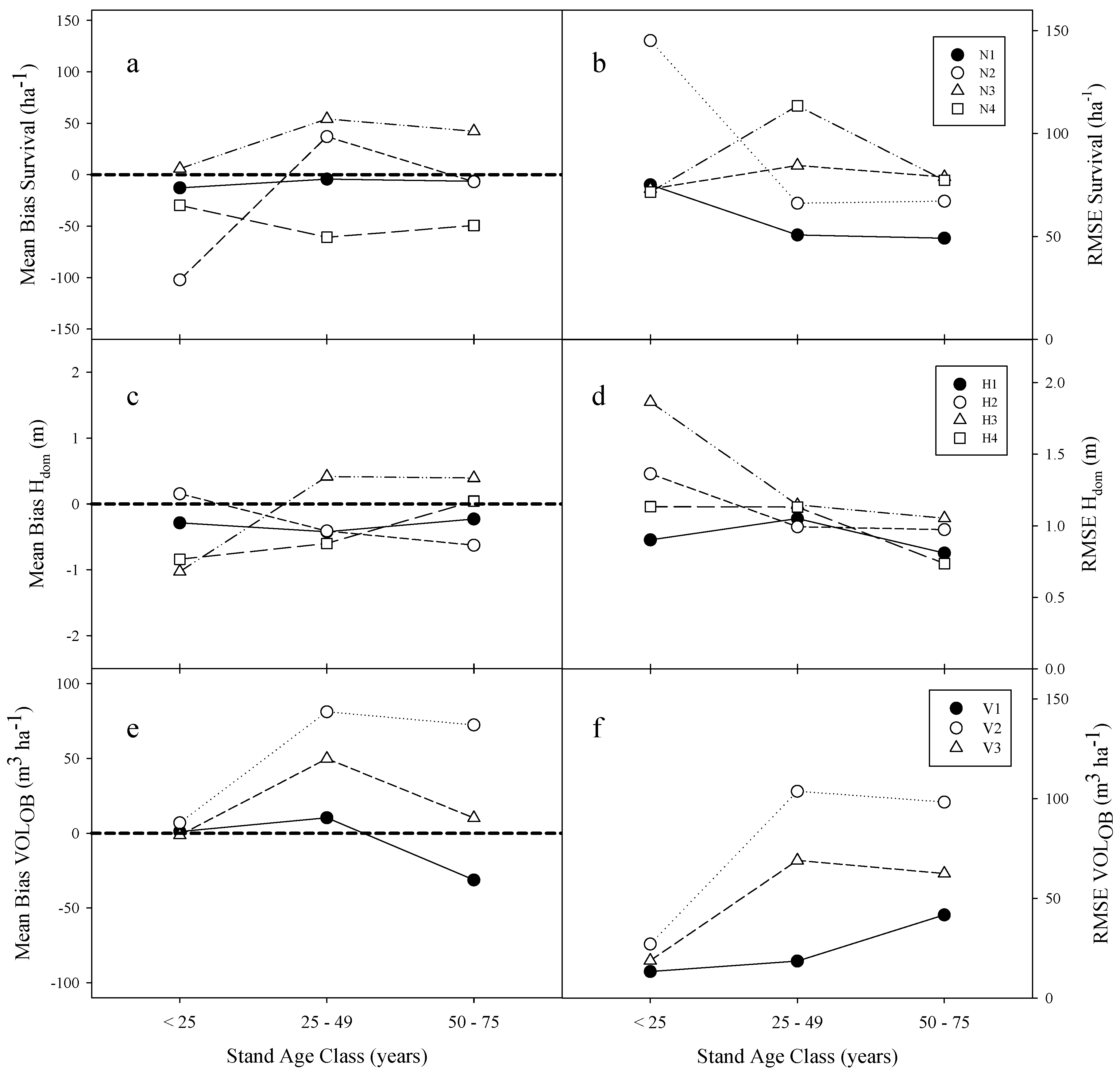
2.3. Model Evaluation
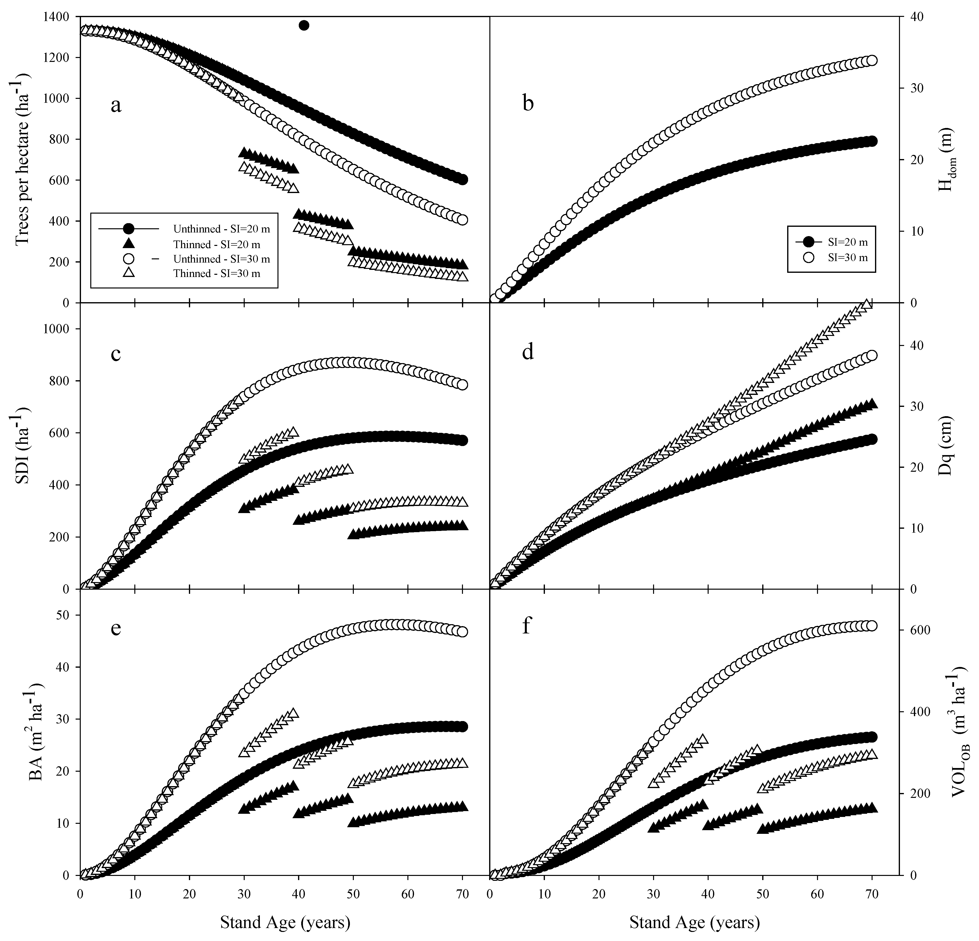
2.4. Model Application Example
3. Results
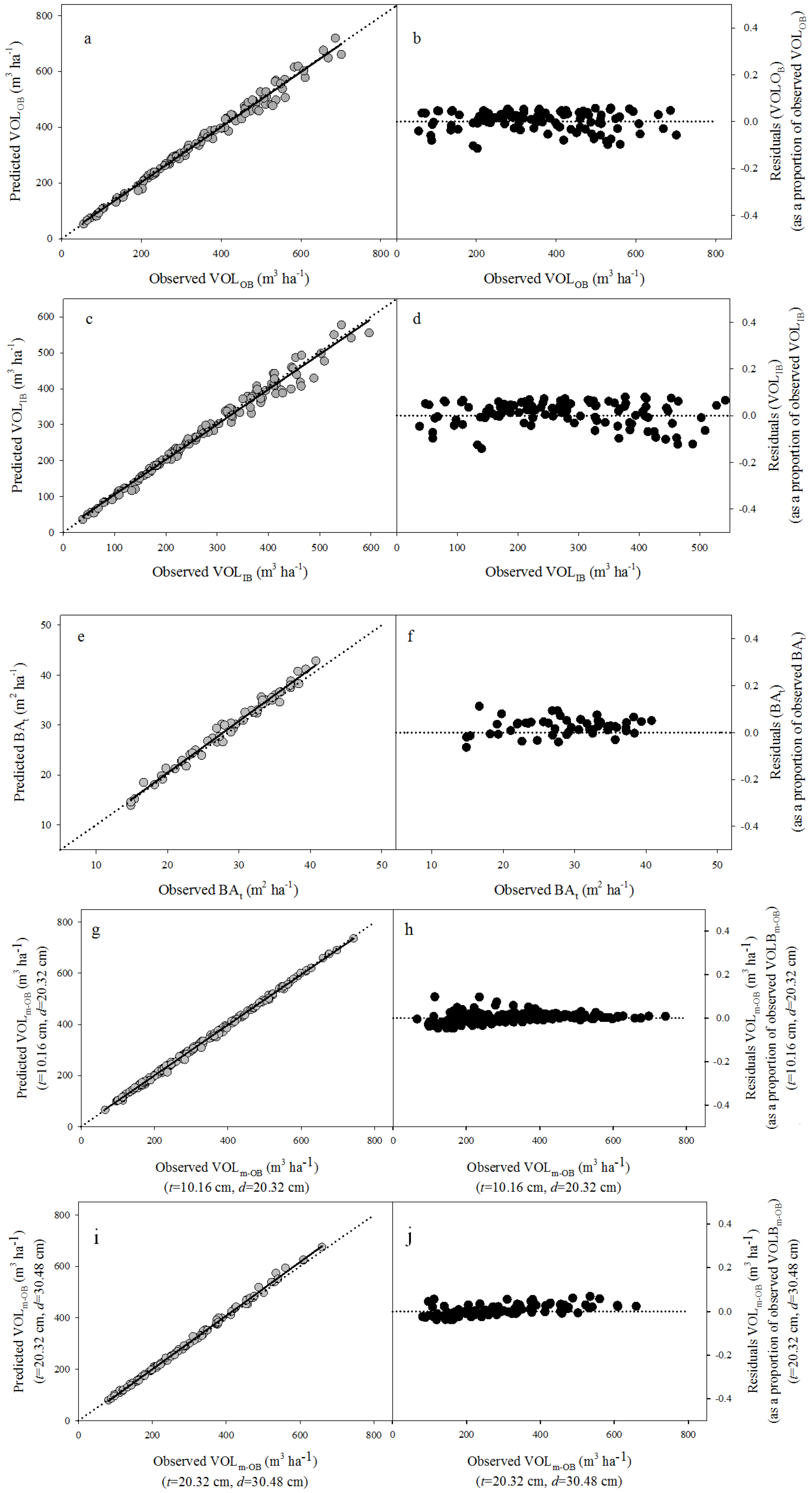
3.1. Model Fitting
| Model | n | Parameter | Parameterestimate | Approx.SE | Approx. Pr > F | VIF | R2 | RMSE | CV% |
|---|---|---|---|---|---|---|---|---|---|
 | 569 | a1 | −0.0369815 | 0.0015463 | <0.0001 | n.a. | 0.998 | 0.87 | 4.1 |
| a2 | 1.2928702 | 0.0454849 | <0.0001 | n.a. | |||||
 | 622 | b1 | −0.0015002 | 0.0006992 | 0.0324 | n.a. | 0.997 | 52.89 | 6.9 |
| b2 | 0.8635401 | 0.1000509 | <0.0001 | n.a. | |||||
 | 725 | c1 * | −4.6484039 | 0.0736689 | <0.0001 | 0 | 0.944 | 1.12 | 3.6 |
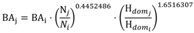
| c2 | 0.4452486 | 0.0064583 | <0.0001 | 1.16 | |||||
| c3 | 1.6526307 | 0.0155728 | <0.0001 | 1.16 | |||||
 | 569 | d1 * | 3.1110579 | 0.0809271 | <0.0001 | 0 | 0.997 | 0.04 | 0.72 |
| d2 | −0.1406022 | 0.0045948 | <0.0001 | 4.41 | |||||
| d3 | 1.1826310 | 0.0040024 | <0.0001 | 2.48 | |||||
| d4 | −2.4435259 | 0.0989071 | <0.0001 | 4.02 | |||||
| d5 | −0.0782880 | 0.0265719 | 0.0033 | 1.49 | |||||
 | 569 | d1 * | 3.0888853 | 0.1026120 | <0.0001 | 0 | 0.996 | 0.05 | 1.0 |
| d2 | −0.1943861 | 0.0058271 | <0.0001 | 4.41 | |||||
| d3 | 1.2580580 | 0.0050738 | <0.0001 | 2.48 | |||||
| d4 | −3.1281571 | 0.1254092 | <0.0001 | 4.02 | |||||
| d5 | −0.098259 | 0.0336921 | 0.0037 | 1.49 | |||||
 | 292 | f1 | −1.5476196 | 0.1881092 | <0.0001 | n.a. | 0.874 | 0.05 | 96.5 |
 | 21,541 | g1 | −1.0385828 | 0.0026438 | <0.0001 | n.a. | 0.990 | 0.07 | 11.1 |
| g2 | 4.2526170 | 0.0147436 | <0.0001 | n.a. | |||||
| g3 | −0.6266850 | 0.0596972 | <0.0001 | n.a. | |||||
| g4 | −0.1246646 | 0.0185442 | <0.0001 | n.a. | |||||
| g5 | 9.1649608 | 0.1878172 | <0.0001 | n.a. | |||||
 | 21,541 | g1 | −1.0537628 | 0.0027184 | <0.0001 | n.a. | 0.990 | 0.07 | 11.2 |
| g2 | 4.2527499 | 0.0148697 | <0.0001 | n.a. | |||||
| g3 | −0.6545719 | 0.0641831 | <0.0001 | n.a. | |||||
| g4 | −0.1365633 | 0.0191092 | <0.0001 | n.a. | |||||
| g5 | 9.3108306 | 0.1971518 | <0.0001 | n.a. |
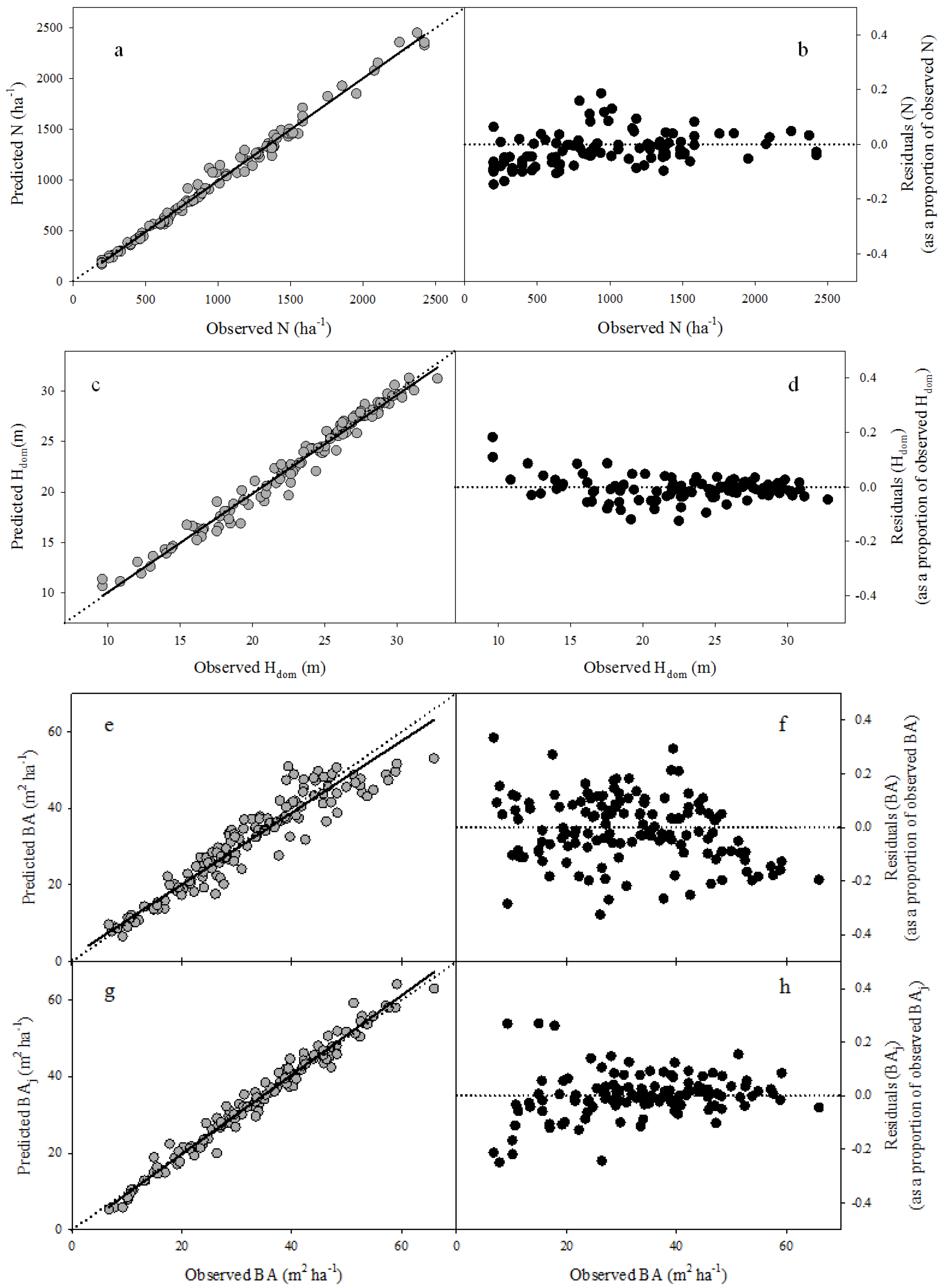
| Variable |  |  | n | MAE | RMSE | Bias | R2 |
|---|---|---|---|---|---|---|---|
| N | 938 | 929 | 120 | 40.3 (4.3) | 53.1 (5.7) | −9.46 (−1.0) | 0.991 |
| Hdom | 23.0 | 22.8 | 111 | 0.6 (2.7) | 0.8 (3.6) | −0.20 (−0.9) | 0.978 |
| BA | 31.5 | 30.8 | 140 | 3.1 (10.0) | 4.2 (13.5) | −0.65 (−2.1) | 0.898 |
| BAj | 33.1 | 33.3 | 120 | 1.9 (5.8) | 2.6 (7.8) | 0.45 (1.4) | 0.970 |
| VOLOB | 340.4 | 341.1 | 115 | 11.9 (3.5) | 16.4 (4.8) | 0.61 (0.2) | 0.990 |
| VOLIB | 269.8 | 270.9 | 115 | 12.3 (4.6) | 17.2 (6.4) | 1.06 (0.4) | 0.984 |
| BAt | 28.5 | 27.9 | 52 | 0.9 (3.1) | 1.1 (3.8) | −0.65 (−2.3) | 0.984 |
| VOLm-OB-t = 10, d = 20 | 137.1 | 138.3 | 70 | 2.5 (1.9) | 4.0 (1.9) | 1.25 (0.9) | 0.999 |
| VOLm-IB-t = 10, d = 20 | 109.9 | 110.8 | 70 | 1.9 (1.7) | 3.0 (1.7) | 0.94 (0.9) | 0.999 |
| VOLm-OB-t = 20, d = 30 | 140.4 | 141.5 | 20 | 7.9 (5.6) | 9.0 (5.6) | 1.14 (0.8) | 0.998 |
| VOLm-IB-t = 20, d = 30 | 115.0 | 114.4 | 20 | 6.3 (5.5) | 7.2 (5.5) | −0.63 (−0.5) | 0.998 |
: mean observed value; : mean predicted value; n: number of observations; MAE: mean absolute error; RMSE: root of mean square error; Bias: absolute bias; R2: coefficient of determination. OB: outside bark; IB: inside bark; t: top diameter (outside bark) merchantability limit (cm); d: dbh threshold limit (cm). Values in parenthesis are percentage relative to observed mean.

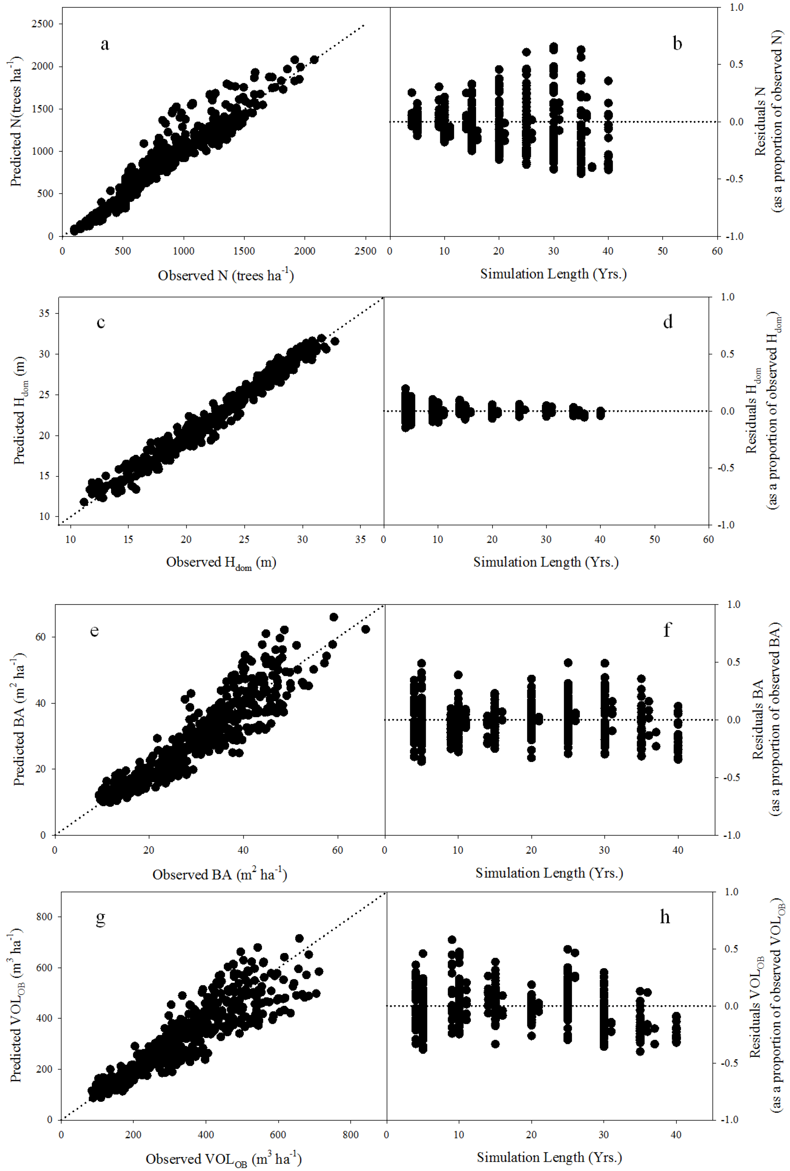
| Variable | Simulation length (yrs.) | | | n | MAE(%) | RMSE(%) | Bias(%) | R2 |
|---|---|---|---|---|---|---|---|---|
| N | 0–20 | 818.5 | 818.3 | 339 | 8.3% | 12.4% | 0.0% | 0.959 |
| 21–40 | 541.1 | 560.9 | 172 | 21.3% | 30.5% | 3.5% | 0.884 | |
| All | 20.9 | 20.9 | 339 | 11.6% | 17.6% | 0.9% | 0.934 | |
| Hdom | 0–20 | 27.2 | 27.2 | 172 | 3.3% | 4.2% | −0.1% | 0.960 |
| 21–40 | 23.0 | 23.0 | 511 | 1.7% | 2.1% | 0.0% | 0.948 | |
| All | 36.1 | 34.9 | 172 | 2.6% | 3.4% | −0.1% | 0.974 | |
| BA | 0–20 | 30.6 | 29.7 | 511 | 9.8% | 13.1% | −2.7% | 0.887 |
| 21–40 | 273.9 | 273.0 | 339 | 15.9% | 19.1% | −3.5% | 0.747 | |
| All | 333.6 | 320.1 | 511 | 12.2% | 16.2% | −3.0% | 0.837 | |
| VOLOB | 0–20 | 818.5 | 818.3 | 339 | 10.4% | 13.6% | −0.3% | 0.895 |
| 21–40 | 541.1 | 560.9 | 172 | 19.6% | 23.2% | −8.7% | 0.557 | |
| All | 20.9 | 20.9 | 339 | 13.2% | 18.3% | −4.2% | 0.839 |
: mean observed value; : mean predicted value; n: number of observations; MAE: mean absolute error (m); RMSE: root of mean square error (m); Bias: absolute bias (m); R2: coefficient of determination. Values of MAE, RSME and Bias are percentage relative to observed mean. 
4. Discussion
Acknowledgments
Conflict of Interest
References
- Frost, C.C. Four centuries of changing landscape patterns in the longleaf pine ecosystem. In The Longleaf Pine Ecosystem: Ecology, Restoration and Management, Proceedings of the 18th Tall Timbers Fire Ecology Conference, Tallahassee, FL, USA, 30 May–2 June 1991; Hermann, S.H., Ed.; Tall Timbers Research Station: Tallahassee, FL, USA, 1993; Volume 18, pp. 17–44. [Google Scholar]
- Frost, C.C. History and future of the longleaf pine ecosystem. In The Longleaf Pine Ecosystem—Ecology, Silviculture and Restoration; Jose, S., Jokela, E.J., Miller, D.L., Eds.; Springer: New York, NY, USA, 2006; pp. 9–48. [Google Scholar]
- Avery, T.R.; Burkhart, H.E. Forest Measurements, 5th ed; McGraw-Hill Inc.: New York, NY, USA, 2002. [Google Scholar]
- Farrar, R.M., Jr. Southern pine site index equations. J. For. 1973, 71, 696–697. [Google Scholar]
- Lohrey, R.E.; Bailey, R.L. Yield Tables and Stand Structure for Unthinned Longleaf Pine Plantations in Louisiana and Texas; Research Paper SO-133 for USDA Forest Service Southern Forest Experiment Station: New Orleans, LA, USA, 1977. [Google Scholar]
- Boyer, W.D. Interim Site-Index Curves for Longleaf Pine Plantations; Research Note SO-261 for USDA Forest Service Southern Forestry Experiment Station: New Orleans, LA, USA, 1980. [Google Scholar]
- Brooks, J.R.; Jack, S.B. A Whole Stand Growth and Yield System for Young Longleaf Pine Plantations in Southwest Georgia; General Technical Report SRS-92 for USDA Forest Service Southern Research Station: Asheville, NC, USA, 2006; pp. 317–318. [Google Scholar]
- VanderShaaf, C.L. LONGLEAF: A Diameter-Distribution Growth and Yield Model and Decision Support System for Unthinned Longleaf Pine Plantations; Texas Forest Service: College Station, TX, USA, 2010. [Google Scholar]
- Goelz, J.C.G.; Leduc, D.J. Long-term studies on development of longleaf pine plantations. In Forests for Our Future, Proceedings of the Third Longleaf Alliance Regional Conference, Alexandria, LA, USA, 16–18 October 2000; Kush, J.S., Ed.; The Longleaf Alliance and Auburn University: Auburn, AL, USA, 2001; pp. 116–118. [Google Scholar]
- Leduc, D.J.; Goelz, J.C.G. A height-diameter curve for longleaf pine plantations in the Gulf Coastal Plain. South. J. Appl. For. 2009, 33, 164–170. [Google Scholar]
- Quicke, H.E.; Meldahl, R.S. Predicting pole classes for longleaf pine based on diameter breast height. South. J. Appl. For. 1992, 16, 79–82. [Google Scholar]
- Clutter, J.L.; Forston, J.C.; Pienaar, L.V.; Brister, G.H.; Bailey, R.L. Timber Management: A Quantitative Approach; Krieger Publishing Company: Malabar, FL, USA, 1983. [Google Scholar]
- Weiskittel, A.R.; Hann, D.W.; Kerhsaw, J.A., Jr.; Vanclay, J.K. Forest Growth and Yield Modeling; Wiley: Oxford, UK, 2011. [Google Scholar]
- Diéguez-Aranda, U.; Castedo Dorado, F.; Álvarez González, J.G.; Rodriguez Soalleiro, R. Modelling mortality of Scots pine (Pinus sylvestris L.) plantations in the northwest of Spain. Eur. J. For. Res. 2005, 124, 143–153. [Google Scholar]
- Diéguez-Aranda, U.; Castedo Dorado, F.; Álvarez González, J.G.; Rojo Alboreca, A. Dynamic growth model for Scots pine (Pinus sylvestris L.) plantations in Galicia (north-western Spain). Ecol. Model. 2006, 191, 225–242. [Google Scholar]
- Zhao, D.; Borders, B.; Wang, M.; Kane, M. Modeling mortality of second-rotation loblolly pine plantations in the Piedmont/Upper Coastal Plain and Lower Coastal Plain of the southern United States. For. Ecol. Manag. 2007, 252, 132–143. [Google Scholar] [CrossRef]
- Burkhart, H.E.; Tomé, M. Modeling Forest Trees and Stands; Springer: New York, NY, USA, 2012. [Google Scholar]
- Borders, B.E. Systems of equations in forest stand modeling. For. Sci. 1989, 35, 548–556. [Google Scholar]
- Gonzalez-Benecke, C.A.; Gezan, S.A.; Martin, T.A.; Cropper, W.P., Jr.; Samuelson, L.; Leduc, D.J. Individual tree diameter, height and volume functions for longleaf pine. For. Sci. 2012. submitted. [Google Scholar]
- Pienaar, L.V. Results and Analysis of a Slash Pine Spacing and Thinning Study in the Southeast Coastal Plain; Technical Report 1995-3 for Plantation Management Research Cooperative (PMRC): University of Georgia, Athens, GA, USA, 1995. [Google Scholar]
- Westfall, J.A.; Burkhart, H.E. Incorporating thinning response into a loblolly pine stand simulator. South. J. Appl. For. 2001, 25, 159–164. [Google Scholar]
- Sharma, M.; Smith, M.; Burkhart, H.E.; Amateis, R.L. Modeling the impact of thinning on height development of dominant and codominant loblolly pine trees. Ann. For. Sci. 2006, 63, 349–354. [Google Scholar] [CrossRef]
- Pienaar, L.V. An approximation of basal area growth after thinning based on growth in unthinned plantations. For. Sci. 1979, 25, 223–232. [Google Scholar]
- Amateis, R.L.; Burkhart, H.E.; Burk, T.E. A ratio approach to predicting merchantable yields of unthinned loblolly pine plantations. For. Sci. 1986, 32, 287–296. [Google Scholar]
- Harrison, W.M.; Borders, B.E. Yield Prediction and Growth Projection for Site-prepared Loblolly Pine Plantations in the Carolinas, Georgia, Alabama and Florida; Technical Report 1996-1 for Plantation Management Research Cooperative (PMRC): University of Georgia, Athens, GA, USA, 1996. [Google Scholar]
- Pienaar, L.V.; Shiver, B.D.; Rheney, J.W. Yield Prediction for Mechanically Site-prepared Slash Pine Plantations in the Southeastern Coastal Plain; Technical Report 1996-3 for Plantation Management Research Cooperative (PMRC): University of Georgia, Athens, GA, USA, 1996. [Google Scholar]
- Yin, R.; Pienaar, L.V.; Aronow, M.E. The productivity and profitability of fiber farming. J. For. 1998, 96, 13–18. [Google Scholar]
- Fox, D.G. Judging air quality model performance. Bull. Am. Meteorol. Soc. 1981, 62, 599–609. [Google Scholar] [CrossRef]
- Willmott, C.; Ackleson, S.; Davis, R.; Feddema, J.; Klink, K.; Legates, D.; O’Donnell, J.; Zhao, W.; Mason, E.G.; Brown, J. Modelling height-diameter relationships of Pinus radiata plantations in Canterbury, New Zealand. N. Z. J. For. 2006, 51, 23–27. [Google Scholar]
- Loague, K.; Green, R.E. Statistical and graphical methods for evaluating solute transport models: Overview and application. J. Contam. Hydrol. 1991, 7, 51–73. [Google Scholar] [CrossRef]
- Kaboyashi, K.; Salam, M.U. Comparing simulated and measured values using mean squared deviation and its components. Agron. J. 2000, 92, 345–352. [Google Scholar]
- Lauer, D.K.; Kush, J.S. A Variable Density Stand Level Growth and Yield Model for Even-aged Natural Longleaf Pine; Special Report No. 10 for Alabama Agricultural Experiment Station Auburn University: Auburn, AL, USA, 2011. [Google Scholar]
- SAS Software, version 9.3; SAS Inc.: Cary, NC, USA, 2011.
- Neter, J.; Kutner, M.H.; Nachtsheim, C.J.; Wasserman, W. Applied Linear Statistical Models, 4th ed; Irwin: Chicago, IL, USA, 1996. [Google Scholar]
- Snowdon, P. A ratio estimator for bias correction in logarithmic regressions. Can. J. For. Res. 1991, 21, 720–724. [Google Scholar] [CrossRef]
- Baskerville, G.L. Use of logarithmic regression in the estimation of plant biomass. Can. J. For. Res. 1972, 2, 49–53. [Google Scholar] [CrossRef]
- Johnson, E.E.; Gjerstad, D. Restoring the overstory of longleaf pine ecosystems. In The Longleaf Pine Ecosystem: Ecology, Silviculture, and Restoration; Jose, S., Jokela, E.J., Miller, D.L., Eds.; Springer: New York, NY, USA, 2006; pp. 271–295. [Google Scholar]
- Outcalt, K.W.; Brockway, D.G. Structure and composition changes following restoration treatments of longleaf pine forests on the Gulf Coastal Plain of Alabama. For. Ecol. Manag. 2010, 259, 1615–1623. [Google Scholar] [CrossRef]
- Farrar, R.M., Jr.; Matney, T.G. A dual growth simulator for natural even-aged stands of longleaf pine in the South’s East Gulf Region. South. J. Appl. For. 1994, 18, 147–155. [Google Scholar]
- Pienaar, L.V.; Rheney, J.W. Yield prediction for mechanically site-prepared slash pine plantations in the southeastern Coastal Plain. South. J. Appl. For. 1993, 17, 163–173. [Google Scholar]
- Clutter, J.L.; Harms, W.R.; Brister, G.H.; Rheney, J.W. Stand Structure and Yields of Site-Prepared Loblolly Pine Plantations in the Lower Coastal Plain of the Carolinas, Georgia and North Florida; General Technical Report SE-27 for USDA Forest Service Southeastern Forest Experiment Station: Asheville, NC, USA, 1984. [Google Scholar]
- Bailey, R.L.; Borders, B.E.; Ware, K.D.; Jones, E.P. A compatible model relating slash pine plantation survival to density, age site index, and type and intensity of thinning. For. Sci. 1985, 31, 180–189. [Google Scholar]
- Dean, T.J.; Jokela, E.J. A density management diagram for slash pine plantations in the lower Coastal Plain. South. J. Appl. For. 1992, 16, 178–185. [Google Scholar]
- Samuelson, L.J.; Butnor, J.; Maier, C.; Stokes, T.A.; Johnsen, K.; Kane, M. Growth and physiology of loblolly pine in response to long-term resource management: Defining growth potential in the southern United States. Can. J. For. Res. 2008, 38, 721–732. [Google Scholar] [CrossRef]
- Jokela, E.J.; Martin, T.A.; Vogel, J.G. Twenty-five years of intensive forest management with southern pines: Important lessons learned. J. For. 2010, 108, 338–347. [Google Scholar]
- Murphy, P.A.; Farrar, R.M., Jr. A New Mortality (or Survival) Function for Longleaf Pine Plantations; General Technical Report SO-74 for U.S. Department of Agriculture Forest Service Southern Research Station: New Orleans, LA, USA, 1988; pp. 427–432. [Google Scholar]
- Beers, B.L.; Bailey, R.L. Yield Stand Structure and Economic Conclusions from a 22-Year-Old Site Preparation Study with Planted Loblolly and Longleaf Pines; General Technical Report SO-54 for U.S. Department of Agriculture Forest Service Southern Research Station: New Orleans, LA, USA, 1985. [Google Scholar]
- Farrar, R.M., Jr.; Boyer, W.D. Managing longleaf pine under the selection system—Promises and problems. In Proceedings of the Sixth Biennial Southern Silvicultural Research Conference, Memphis, TN, USA, 30 October–1 November 1990; Coleman, S.S., Neary, D.G., Eds.; USDA Forest Service Southeastern Forest Experiment Station: New Orleans, LA, USA, 1991; pp. 357–368. [Google Scholar]
- Jack, S.B.; Mitchell, R.J.; Pecot, S.D. Silvicultural Alternatives in a Longleaf Pine/Wiregrass Woodland in Southwest Georgia: Understory Hardwood Response to Harvest-created Gaps; General Technical Report SRS-92 for USDA Forest Service Southern Research Station: Asheville, NC, USA, 2006; pp. 85–89. [Google Scholar]
© 2012 by the authors; licensee MDPI, Basel, Switzerland. This article is an open-access article distributed under the terms and conditions of the Creative Commons Attribution license (http://creativecommons.org/licenses/by/3.0/).
Share and Cite
Gonzalez-Benecke, C.A.; Gezan, S.A.; Leduc, D.J.; Martin, T.A.; Cropper, W.P., Jr.; Samuelson, L.J. Modeling Survival, Yield, Volume Partitioning and Their Response to Thinning for Longleaf Pine Plantations. Forests 2012, 3, 1104-1132. https://doi.org/10.3390/f3041104
Gonzalez-Benecke CA, Gezan SA, Leduc DJ, Martin TA, Cropper WP Jr., Samuelson LJ. Modeling Survival, Yield, Volume Partitioning and Their Response to Thinning for Longleaf Pine Plantations. Forests. 2012; 3(4):1104-1132. https://doi.org/10.3390/f3041104
Chicago/Turabian StyleGonzalez-Benecke, Carlos A., Salvador A. Gezan, Daniel J. Leduc, Timothy A. Martin, Wendell P. Cropper, Jr., and Lisa J. Samuelson. 2012. "Modeling Survival, Yield, Volume Partitioning and Their Response to Thinning for Longleaf Pine Plantations" Forests 3, no. 4: 1104-1132. https://doi.org/10.3390/f3041104