Exploiting Growing Stock Volume Maps for Large Scale Forest Resource Assessment: Cross-Comparisons of ASAR- and PALSAR-Based GSV Estimates with Forest Inventory in Central Siberia


 ,
,
Abstract
: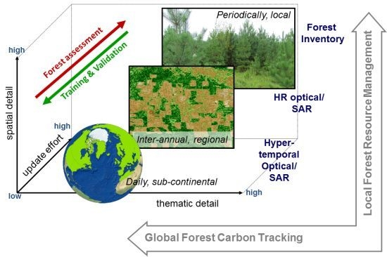
1. Introduction

- -
- cross-compare GSV maps derived from ALOS-PALSAR (25 m, L-band) data and ENVISAT ASAR (1 km, C-band) backscatter data with updated forest inventory maps for test sites in Central Siberia, and
- -
- analyze the effects of forest cover type and landscape fragmentation on the spatial congruence of multi-scale GSV maps.
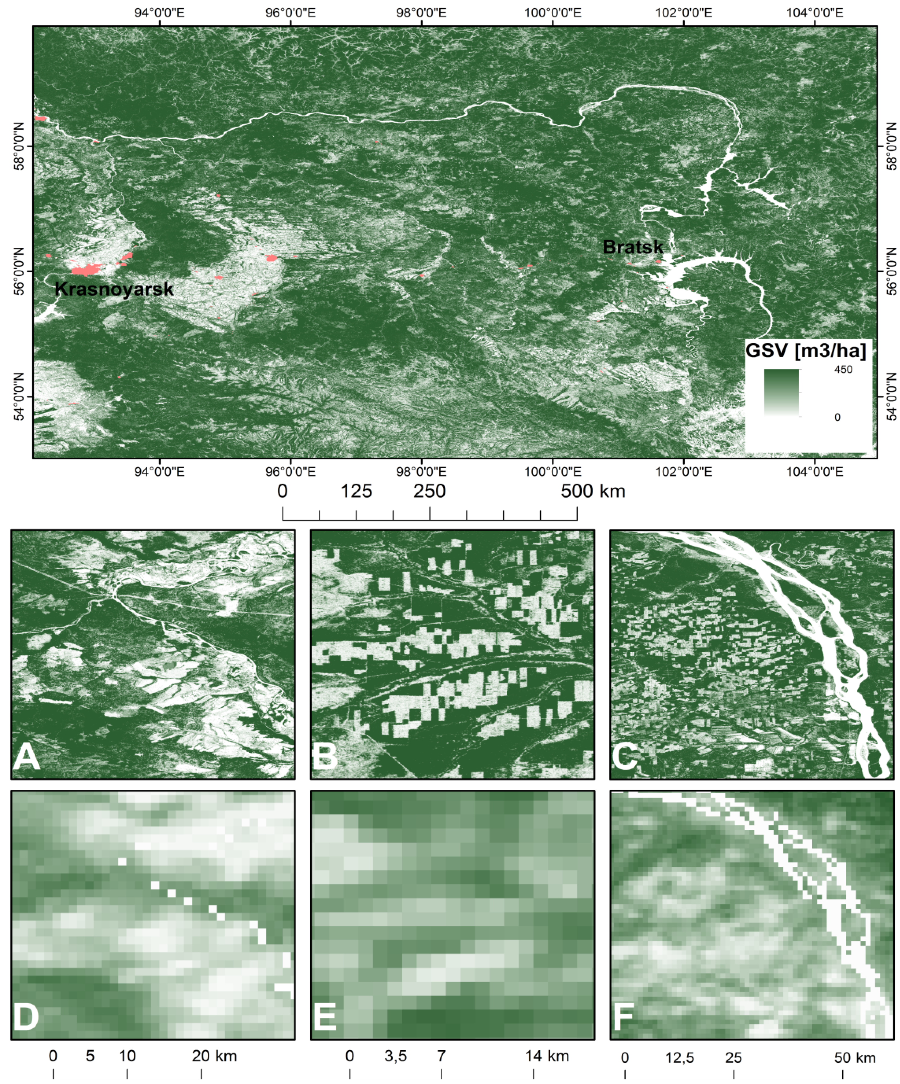
2. Study Area and Data
2.1. Forest Inventory Data of Central Siberia Test Sits

| Site № | Site Name (Forest Management Area) | Area, ha | Number of EFIU | Region |
|---|---|---|---|---|
| 1 | Kazachinsk and Bolshemurtinsk | 943,494 | 51,804 | Krasnoyarsk Kray |
| 2 | Abansk and Dolgomostovsk | 727,139 | 45,424 | Krasnoyarsk Kray |
| 3 | Padunsk | 378,996 | 23,408 | Irkutsk Oblast |
| Total | 2,049,629 | 120,636 |

2.2. ALOS PALSAR
2.3. ENVISAT ASAR
2.4. MODIS
3. Methods
3.1. Update and Quality Assessment of Forest Inventory Data
3.2. ALOS PALSAR Estimates of GSV
3.3. ENVISAT ASAR Estimates of GSV
3.4. Land Cover Mapping
3.5. GSV Cross-Comparisons and Fragmentation Analyses
| Metric Name | Description |
|---|---|
Mean Patch Size  | Mean patch size indicates the mean size of all patches for a specific class in the landscape [44]. |
| Shape index SHAPE = (0.25 p_ij)/√(a_ij) | “Shape index measures the complexity of patch shape compared to a standard shape. Mean shape index measures the average patch shape, or the average perimeter-to-area ratio, for a particular patch type (class) or for all patches in the landscape” [44]; pij = perimeter (m) of patch ij a = area (m ) of patch ij. |
Total (Class) Area  | “Total area equals the sum of the areas (m2) of all patches of the corresponding patch type, a measure of landscape composition; specifically, how much of the landscape is comprised of a particular patch type” [44]; a = area (m) of patch ij. |
Splitting Index  | “Fragmentation indices based on the ability of two animals to get connected in a landscape; splitting index is defined as the number of patches in a landscape when dividing the total region into parts of equal size in such a way that this new configuration leads to the same degree of landscape division. Effective mesh size denotes the size of the areas when the region under investigation is divided into areas with the same degree of landscape division [45]; a = area (m) of patch ij. 2; A = total landscape area (m) |
Effective Mesh Size  |
4. Results
4.1. Forest Inventory Update

| Test Site | Padunsk | Bolshemurtinsk | Kazachinsk | Dolgomostovsk | Abansk | |||||
|---|---|---|---|---|---|---|---|---|---|---|
| Land cover type | Avg m3/ha | Max m3/ha | Avg m3/ha | Max m3/ha | Avg m3/ha | Max m3/ha | Avg m3/ha | Max m3/ha | Avg m3/ha | Max m3/ha |
| Birch | 109 | 280 | 122 | 320 | 118 | 270 | 103 | 320 | 96 | 270 |
| Scots Pine | 173 | 480 | 171 | 440 | 185 | 410 | 165 | 420 | 158 | 430 |
| Aspen | 132 | 330 | 169 | 450 | 149 | 380 | 157 | 380 | 178 | 340 |
| Spruce | 142 | 290 | 202 | 420 | 178 | 380 | 175 | 410 | 140 | 330 |
| Fir | 147 | 310 | 200 | 470 | 169 | 330 | 229 | 360 | 186 | 340 |
| Larch | 178 | 400 | 156 | 350 | 149 | 290 | 170 | 380 | 166 | 310 |
| Siberian pine | 102 | 400 | 269 | 520 | 240 | 400 | 191 | 360 | 275 | 450 |
| Willow | 39 | 90 | 39 | 90 | 17 | 35 | 49 | 60 | 26 | 40 |
| Disturbances | Stands | Area (ha) | Stands | Area (ha) | Stands | Area (ha) | Stands | Area (ha) | Stands | Area (ha) |
| Actual cutting (2010–2011) | 0 | 0 | 10 | 197 | 23 | 316 | 6 | 57 | 5 | 29 |
| Clear-cut (2002–2009) | 475 | 5,416 | 649 | 15,718 | 160 | 2,618 | 181 | 1,408 | 526 | 3,692 |
| Burned area (2002–2009) | 67 | 1,608 | 5 | 458 | 7 | 336 | 42 | 961 | 99 | 2,364 |
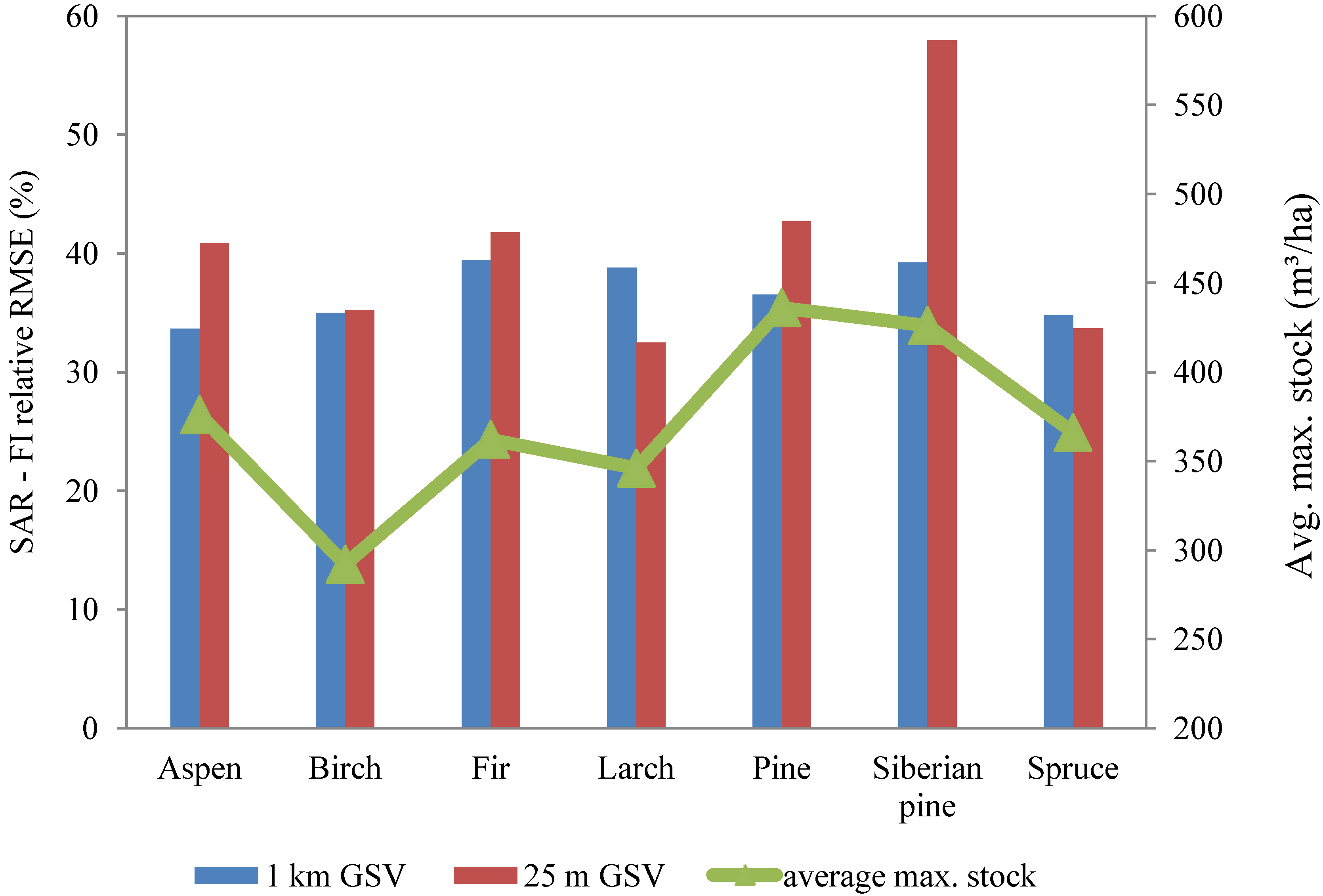
4.2. Assessment of Retrieved Forest GSV with Respect to Forest Inventory Data
| Site | 1 | 2 | 3 | Total Mean | ||||
|---|---|---|---|---|---|---|---|---|
| Overall for Test Sites | 1 km | 25 m | 1 km | 25 m | 1 km | 25 m | 1 km | 25 m |
| R | 0.34 | 0.39 | 0.60 | 0.55 | 0.30 | 0.54 | 0.41 | 0.49 |
| RMSE (%) | 35.00 | 40.71 | 28.39 | 35.06 | 38.63 | 42.44 | 34.01 | 39.40 |
| RMSE (m3/ha) | 58.80 | 68.40 | 47.70 | 58.90 | 64.90 | 71.30 | 57.13 | 66.20 |
| RMSE (m3/ha) Relative RMSE (%) * | 1 km | 25 m | 1 km | 25 m | 1 km | 25 m | 1 km | 25 m |
| Aspen | 62.50 | 70.70 | 46.90 | 66.00 | 60.10 | 69.20 | 56.50 | 68.63 |
| 37.20 | 42.08 | 27.92 | 39.29 | 35.77 | 41.19 | 33.63 | 40.85 | |
| Birch | 59.10 | 60.30 | 48.00 | 55.00 | 69.10 | 62.00 | 58.73 | 59.10 |
| 35.18 | 35.89 | 28.57 | 32.74 | 41.13 | 36.90 | 34.96 | 35.18 | |
| Fir | 57.70 | 78.00 | 46.00 | 65.90 | 94.90 | 66.50 | 66.20 | 70.13 |
| 34.35 | 46.43 | 27.38 | 39.23 | 56.49 | 39.58 | 39.40 | 41.75 | |
| Larch | 57.40 | 53.10 | 75.10 | 55.00 | 63.00 | 55.60 | 65.17 | 54.57 |
| 34.17 | 31.61 | 44.70 | 32.74 | 37.50 | 33.10 | 38.79 | 32.48 | |
| Pine | 76.10 | 72.30 | 47.70 | 63.70 | 60.20 | 79.10 | 61.33 | 71.70 |
| 45.30 | 43.04 | 28.39 | 37.92 | 35.83 | 47.08 | 36.51 | 42.68 | |
| Siberian pine | 52.10 | 92.50 | 53.10 | 99.80 | 92.50 | 99.80 | 65.90 | 97.37 |
| 31.01 | 55.06 | 31.61 | 59.40 | 55.06 | 59.40 | 39.23 | 57.96 | |
| Spruce | 44.20 | 62.30 | 42.30 | 52.40 | 88.70 | 55.10 | 58.40 | 56.60 |
| 26.31 | 37.08 | 25.18 | 31.19 | 52.80 | 32.80 | 34.76 | 33.69 | |

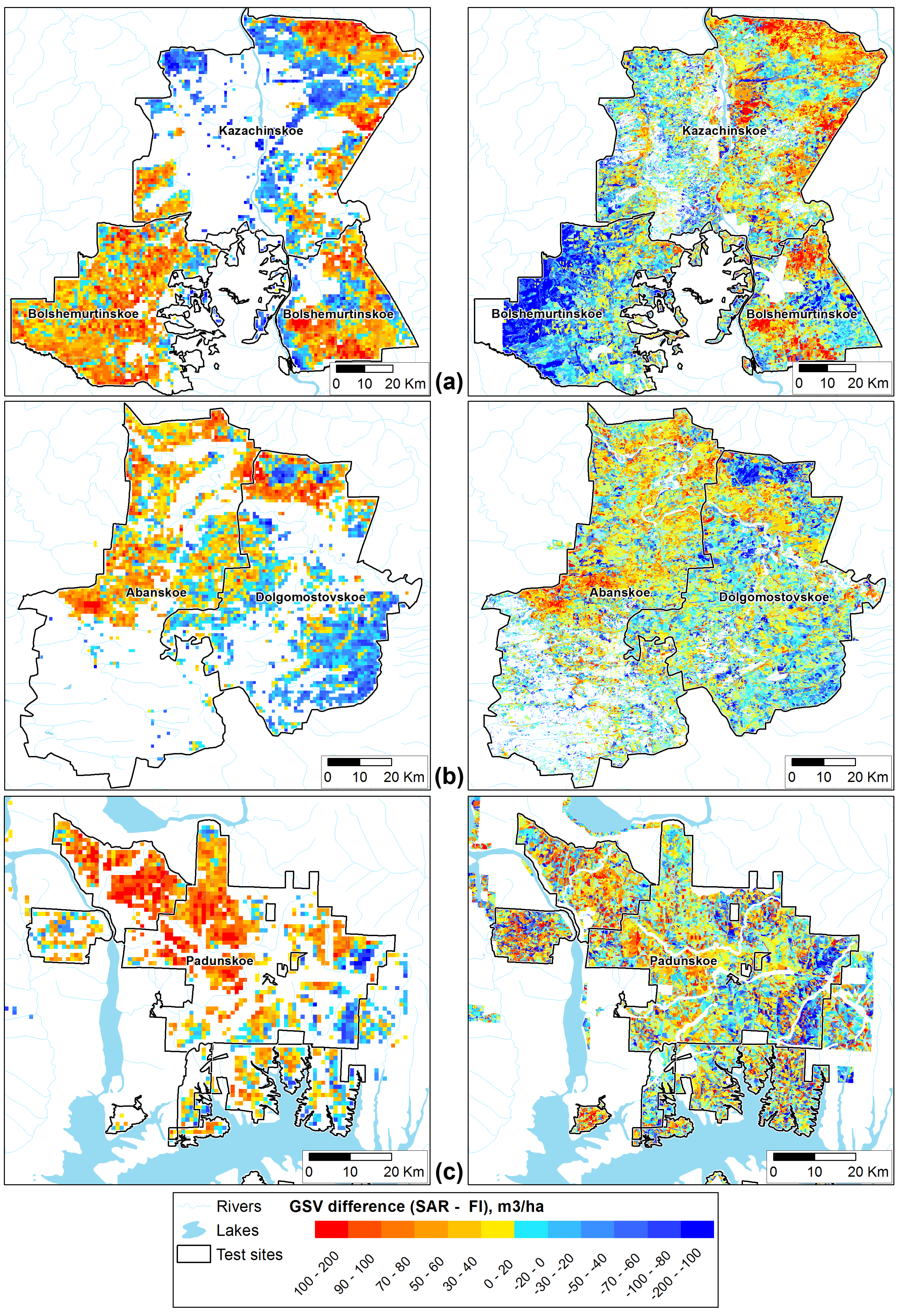
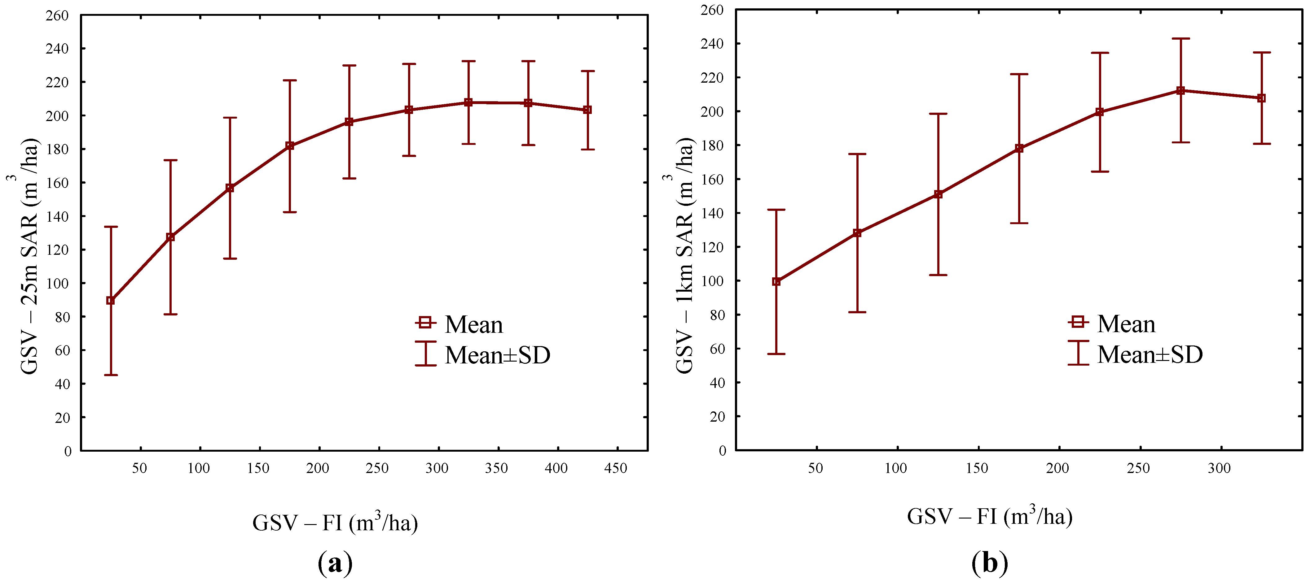
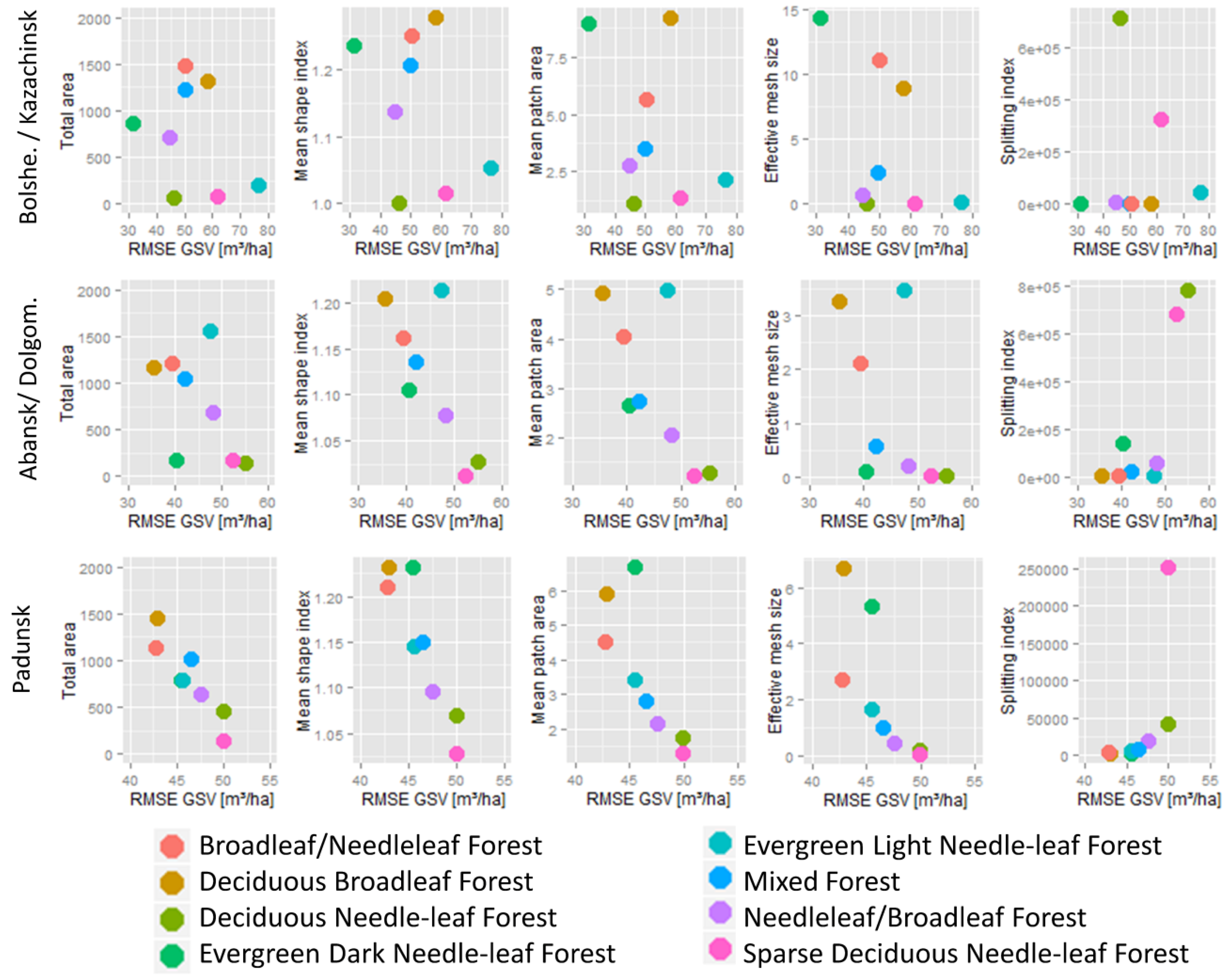
4.3. Cross-Comparison of SAR-Based GSV Datasets


4.4. Land Cover Distribution Effects on Growing Stock Volume Estimation and Map Congruity

5. Discussion
5.1. Determinants of Sensor Type and GSV Retrieval Methods
5.2. Determinants of Forest Cover Type and Distribution
5.3. Fostering SAR-Based GSV Assessments for Central Siberian Forest Inventory Support

6. Conclusions
Acknowledgments
Author Contributions
Conflicts of Interest
References
- Shvidenko, A.; Schepaschenko, D.; Nilsson, S.; Bouloui, Y. Semi-empirical models for assessing biological productivity of Northern Eurasian forests. Ecol. Model. 2007, 204, 163–179. [Google Scholar] [CrossRef]
- Gusti, M.; Jonas, M. Terrestrial full carbon account for Russia: Revised uncertainty estimates and their role in a bottom-up/top-down accounting exercise. Clim. Chang. 2010, 103, 159–174. [Google Scholar] [CrossRef]
- Dolman, J.; Shvidenko, A.; Schepaschenko, D.; Ciais, P.; Tchebakova, N.; Chen, T.; van der Molen, M.K.; Belelli Marchesini, L.; Maximov, T.C.; Maksyutov, S.; Schulze, E.-D. An Estimate of the Terrestrial Carbon Budget of Russia Using Inventory-Based, Eddy Covariance and Inversion Methods. Biogeosciences 2012, 9, 5323–5340. [Google Scholar] [CrossRef] [Green Version]
- Shvidenko, A.; Schepaschenko, D. Russia faces tough climate change challenges. Options 2011, 18–19. [Google Scholar]
- Schepaschenko, D.; See, L.; Fritz, S.; McCallum, I.; Christian, S.; Perger, C.; Baccini, A.; Gallaun, H.; Kindermann, G.; Kraxner, F.; et al. Observing forest biomass globally. Earthzine 2012. [Google Scholar]
- Shvidenko, A.; Schepaschenko, D.; McCallum, I.; Nilsson, S. Can the uncertainty of full carbon accounting of forest ecosystems be made acceptable to policymakers? Clim. Chang. 2010, 103, 137–157. [Google Scholar] [CrossRef]
- Gustafson, E.J.; Shvidenko, A.Z.; Sturtevant, B.R.; Scheller, R.M. Predicting global change effects on forest biomass and composition in south-central Siberia. Ecol. Appl. 2010, 20, 700–715. [Google Scholar] [CrossRef]
- Pereira, H.M.; Ferrier, S.; Walters, M.; Geller, G.N.; Jongman, R.H.G.; Scholes, R.J.; Bruford, M.W.; Brummitt, N.; Butchart, S.H.M.; Cardoso, A.C.; et al. Essential Biodiversity Variables. Science 2013, 339, 277–278. [Google Scholar] [CrossRef] [Green Version]
- Houghton, R.A.; Butman, D.; Bunn, A.G.; Krankina, O.N.; Schlesinger, P.; Stone, T.A. Mapping Russian forest biomass with data from satellites and forest inventories. Environ. Res. Lett. 2007, 2, 045032. [Google Scholar] [CrossRef]
- McRoberts, R.E.; Gobakken, T.; Næsset, E. Post-stratified estimation of forest area and growing stock volume using lidar-based stratifications. Remote Sens. Environ. 2012, 125, 157–166. [Google Scholar] [CrossRef]
- Powell, S.L.; Cohen, W.B.; Healey, S.P.R.; Kennedy, E.; Moisen, G.G.; Pierce, K.B.; Ohmann, J.L. Quantification of live aboveground forest biomass dynamics with Landsat time-series and field inventory data: A comparison of empirical modeling approaches. Remote Sens. Environ. 2010, 114, 1053–1068. [Google Scholar] [CrossRef]
- Tomppo, E.O.; Gagliano, C.; de Natale, F.; Katila, M.; McRoberts, R.E. Predicting categorical forest variables using an improved k-Nearest Neighbour estimator and Landsat imagery. Remote Sens. Environ. 2009, 113, 500–517. [Google Scholar] [CrossRef]
- Tomppo, E.; Nilsson, M.; Rosengren, M.; Aalto, P.; Kennedy, P. Simultaneous use of Landsat-TM and IRS-1C WiFS data in estimating large area tree stem volume and aboveground biomass. Remote Sens. Environ. 2002, 82, 156–171. [Google Scholar] [CrossRef]
- Santoro, M.; Beer, C.; Cartus, O.; Schmullius, C.; Shvidenko, A.; McCallum, I.; Wegmüller, U.; Wiesmann, A. Retrieval of growing stock volume in boreal forest using hyper-temporal series of Envisat ASAR ScanSAR backscatter measurements. Remote Sens. Environ. 2010, 115, 490–507. [Google Scholar]
- Santoro, M.; Cartus, O.; Fransson, J.; Shvidenko, A.; McCallum, I.; Hall, R.; Beaudoin, A.; Beer, C.; Schmullius, C. Estimates of forest growing stock volume for Sweden, central Siberia, and québec using envisat advanced synthetic aperture radar backscatter data. Remote Sens. 2013, 5, 4503–4532. [Google Scholar] [CrossRef]
- Goetz, S.J.; Baccini, A.; Laporte, N.T.; Johns, T.; Walker, W.; Kellndorfer, J.; Houghton, R.; Sun, M. Mapping and monitoring carbon stocks with satellite observations: A comparison of methods. Carbon Balance Manag. 2009, 4. [Google Scholar] [CrossRef]
- Cartus, O.; Kellndorfer, J.; Rombach, M.; Walker, W. Mapping canopy height and growing stock volume using airborne lidar, ALOS PALSAR and landsat ETM+. Remote Sens. 2012, 4, 3320–3345. [Google Scholar] [CrossRef]
- De Grandi, G.D.; Bouvet, A.; Lucas, R.M.; Shimada, M.; Monaco, S.; Rosenqvist, A. The KC PALSAR mosaic of the African continent: Processing issues and first thematic results. IEEE Trans. Geosci. Remote Sens. 2011, 49, 3593–3610. [Google Scholar]
- Santoro, M.; Schmullius, C.; Pathe, C.; Schwilk, J. Pan-boreal mapping of forest growing stock volume using hyper-temporal Envisat ASAR ScanSAR backscatter data. In Proceedings of the 2012 IEEE International on Geoscience Remote Sensing Symposium (IGARSS), Munich, Germany, 22–27 July 2012; pp. 7204–7207.
- Seifert, F.M. GlobBiomass—User Consultation Meeting. 2012. Available online: http://due.esrin.esa.int/meetings/meetings283.php (accessed on 25 July 2013).
- Corona, P. Integration of forest mapping and inventory to support forest management. iForest—Biogeosci. For. 2010, 3, 59–64. [Google Scholar] [CrossRef]
- Wulder, M.A.; White, J.C.; Fournier, R.A.J.; Luther, E.; Magnussen, S. Spatially explicit large area biomass estimation: Three approaches using forest inventory and remotely sensed imagery in a GIS. Sensors 2008, 8, 529–560. [Google Scholar]
- Blackard, J.; Finco, M.; Helmer, E.; Holden, G.; Hoppus, M.; Jacobs, D.; Lister, A.; Moisen, G.; Nelson, M.; Riemann, R. Mapping U.S. forest biomass using nationwide forest inventory data and moderate resolution information. Remote Sens. Environ. 2008, 112, 1658–1677. [Google Scholar] [CrossRef]
- Ryan, B. Introduction to GEO. In Proceedings of the UNFCCC COP-18, Doha, Qatar, 26 November–7 December 2012.
- Minayeva, L.Y. Forest inventory regulations of Russia. Mil. Tiprg. 1995, 1, 274. [Google Scholar]
- Santoro, M.; Eriksson, L.; Askne, J.; Schmullius, C. Assessment of stand-wise stem volume retrieval in boreal forest from JERS-1 L-band SAR backscatter. Int. J. Remote Sens. 2006, 27, 3425–3454. [Google Scholar] [CrossRef]
- Shimada, M.; Ohtaki, T. Generating large-scale high-quality SAR mosaic datasets: Application to PALSAR data for global monitoring. IEEE J. Sel. Top. Appl. Earth Obs. Remote Sens. 2010, 3, 637–656. [Google Scholar] [CrossRef]
- Rosenqvist, A.; Ogawa, T.; Shimada, M.; Igarashi, T. Initiating the ALOS Kyoto & Carbon Initiative. In Proceedings of the IEEE 2001 International Geoscience and Remote Sensing Symposium on IGARSS 2001 Scanning the Present and Resolving the Future, Sydney, NSW, Australia, 9–13 July 2001; Volume 1, pp. 546–548.
- Bartalev, S.A.; Belward, A.S.; Erchov, D.V.; Isaev, A.S. A new SPOT4-VEGETATION derived land cover map of Northern Eurasia. Int. J. Remote Sens. 2003, 24, 1977–1982. [Google Scholar] [CrossRef]
- Zharko, V.O.; Bartalev, S.A.; Egorov, V.A. Evaluation of forest tree species composition based on the analysis of their seasonal reflectance dynamic using satellite data. (in Russian). In Proceedings of the Tenth Annual All Russian Open Conference Actual Problems in Remote Sensing of the Earth from Space, Moscow, Russia, 12–16 November 2012; p. 386.
- FFSR. Manual on forest inventory and planning in forest fund of Russia. Part 1. Organization of forest inventory and field works; Federal Forest Service of Russia: Moscow, Russia, 1995; p. 174.
- Prasad, M.; Iverson, L.R.; Liaw, A. Newer classification and regression tree techniques: Bagging and random forests for ecological prediction. Ecosystem 2006, 9, 181–199. [Google Scholar] [CrossRef]
- Gislason, P.; Benediktsson, J.; Sveinsson, J. Random Forests for land cover classification. Pattern Recognit. Lett. 2006, 27, 294–300. [Google Scholar] [CrossRef]
- Cutler, D.R.; Edwards, T.C.; Beard, K.H.; Cutler, A.; Hess, K.T.; Gibson, J.; Lawler, J.J. Random forests for classification in ecology. Ecology 2007, 88, 2783–2792. [Google Scholar] [CrossRef]
- Hüttich, C.; Herold, M.; Strohbach, B.J.; Dech, S. Integrating in situ-, Landsat-, and MODIS data for mapping in Southern African savannas: Experiences of LCCS-based land-cover mapping in the Kalahari in Namibia. Environ. Monit. Assess. 2010, 176, 531–547. [Google Scholar]
- Simard, M.; Pinto, N.; Fisher, J.B.; Baccini, A. Mapping forest canopy height globally with spaceborne lidar. J. Geophys. Res. 2011, 116, 1–12. [Google Scholar]
- Carreiras, J.; Melo, J.; Vasconcelos, M. Estimating the above-ground biomass in Miombo savanna woodlands (Mozambique, East Africa) using L-band synthetic aperture radar data. Remote Sens. 2013, 5, 1524–1548. [Google Scholar] [CrossRef]
- Breiman, L.; Friedman, J.H.; Olshen, R.A.; Stone, C.J. Classification and Regression Trees; CRC Press: Boca Raton, FL, USA, 1984; p. 368. [Google Scholar]
- Imhoff, M.L. Radar backscatter and biomass saturation: Ramifications for global biomass inventory. IEEE Trans. Geosci. Remote Sens. 1995, 33, 511–518. [Google Scholar] [CrossRef]
- Wagner, W. Large-scale mapping of boreal forest in SIBERIA using ERS tandem coherence and JERS backscatter data. Remote Sens. Environ. 2003, 85, 125–144. [Google Scholar] [CrossRef]
- Santoro, M.; Shvidenko, A.; Mccallum, I.; Askne, J.; Schmullius, C. Properties of ERS-1/2 coherence in the Siberian boreal forest and implications for stem volume retrieval. Remote Sens. Environ. 2007, 106, 154–172. [Google Scholar] [CrossRef]
- Bartalev, S.A.; Egorov, V.A.; Loupian, E.A.; Khvostikov, S.A. A new locally-adaptive classificationmethod LAGMA for large-scale land cover mapping using remote-sensing data. Remote Sens. Lett. 2014, 5, 55–64. [Google Scholar] [CrossRef]
- Bartalev, S.A.; Egorov, V.A.; Ershov, D.V.; Isaev, A.S.; Loupian, E.A.; Plotnikov, D.E.; Uvarov, I.A. The vegetation mapping over Russia using MODIS spectroradiometer satellite data. Contemp. Earth Remote Sens. Sp. 2011, 8, 285–302. [Google Scholar]
- McGarigal, K.; Cushman, S.A.; Neel, M.C.; Ene, E. FRAGSTATS: Spatial pattern analysis program for categorical maps. In Computer Software Program Produced by the Authors at the University of Massachusetts; University of Massachusets: Amherst, United States of America, 2002; p. 171. [Google Scholar]
- Jaeger, J.A.G. Landscape division, splitting index, and effective mesh size: New measures of landscape fragmentation. Landsc. Ecol. 2000, 15, 115–130. [Google Scholar] [CrossRef]
- Rauste, Y. Multi-temporal JERS SAR data in boreal forest biomass mapping. Remote Sens. Environ. 2005, 97, 263–275. [Google Scholar] [CrossRef]
- Thiel, C.; Schmullius, C. Investigating the impact of freezing on the ALOS PALSAR InSAR phase over Siberian forests. Remote Sens. Lett. 2013, 4, 900–909. [Google Scholar] [CrossRef]
- Kasischke, E.S.; Tanase, M.A.; Bourgeau-Chavez, L.L.; Borr, M. Soil moisture limitations on monitoring boreal forest regrowth using spaceborne L-band SAR data. Remote Sens. Environ. 2011, 115, 227–232. [Google Scholar] [CrossRef]
- JAXA. New Global 50 m-Resolution PALSAR Mosaic and Forest/Non-Forest Map (2007–2010). Available online: http://www.eorc.jaxa.jp/ALOS/en/palsar_fnf/fnf_index.htm (accessed on 12 May 2014).
- Kuemmerle, T.; Chaskovskyy, O.; Knorn, J.; Radeloff, V.C.; Kruhlov, I.; Keeton, W.S.; Hostert, P. Forest cover change and illegal logging in the Ukrainian Carpathians in the transition period from 1988 to 2007. Remote Sens. Environ. 2009, 113, 1194–1207. [Google Scholar]
- Hain, H.; Ahas, R. The structure and estimated extent of illegal forestry in Estonia 1998–2003. Int. For. Rev. 2005, 7, 90–100. [Google Scholar]
- Le Toan, T.; Quegan, S.; Davidson, M.W.J.; Balzter, H.; Paillou, P.; Papathanassiou, K.; Plummer, S.; Rocca, F.; Saatchi, S.; Shugart, H.; et al. The BIOMASS mission: Mapping global forest biomass to better understand the terrestrial carbon cycle. Remote Sens. Environ. 2011, 115, 2850–2860. [Google Scholar] [CrossRef]
© 2014 by the authors; licensee MDPI, Basel, Switzerland. This article is an open access article distributed under the terms and conditions of the Creative Commons Attribution license (http://creativecommons.org/licenses/by/3.0/).
Share and Cite
Hüttich, C.; Korets, M.; Bartalev, S.; Zharko, V.; Schepaschenko, D.; Shvidenko, A.; Schmullius, C. Exploiting Growing Stock Volume Maps for Large Scale Forest Resource Assessment: Cross-Comparisons of ASAR- and PALSAR-Based GSV Estimates with Forest Inventory in Central Siberia. Forests 2014, 5, 1753-1776. https://doi.org/10.3390/f5071753
Hüttich C, Korets M, Bartalev S, Zharko V, Schepaschenko D, Shvidenko A, Schmullius C. Exploiting Growing Stock Volume Maps for Large Scale Forest Resource Assessment: Cross-Comparisons of ASAR- and PALSAR-Based GSV Estimates with Forest Inventory in Central Siberia. Forests. 2014; 5(7):1753-1776. https://doi.org/10.3390/f5071753
Chicago/Turabian StyleHüttich, Christian, Mikhail Korets, Sergey Bartalev, Vasily Zharko, Dmitry Schepaschenko, Anatoly Shvidenko, and Christiane Schmullius. 2014. "Exploiting Growing Stock Volume Maps for Large Scale Forest Resource Assessment: Cross-Comparisons of ASAR- and PALSAR-Based GSV Estimates with Forest Inventory in Central Siberia" Forests 5, no. 7: 1753-1776. https://doi.org/10.3390/f5071753