Article

Quantifying the Effects of Biomass Market Conditions and Policy Incentives on Economically Feasible Sites to Establish Dedicated Energy Crops

1
Department of Geography, Room 304, Burchfiel Geography Building, University of Tennessee, Knoxville, TN 37996, USA
2
Department of Forestry, University of Kentucky, Thomas Poe Cooper Building, Lexington, KY 40546, USA
*
Author to whom correspondence should be addressed.
Forests 2015, 6(11), 4168-4190; https://doi.org/10.3390/f6114168
Submission received: 11 August 2015 / Revised: 12 October 2015 / Accepted: 12 November 2015 / Published: 18 November 2015

Abstract

:
This study used a spatially-explicit model to identify the amount and spatial distribution of economically feasible sites for establishing dedicated energy crops under various market and policy scenarios. A sensitivity analysis was performed for a biomass market with different discount rates and biomass prices as well as policy scenarios including propriety tax exemption, carbon offset payments, and the inclusion of farmland for biomass production. The model was applied to a four-county study area in Kentucky representing conditions commonly found in the Ohio River Valley. Results showed that both biomass price and discount rate have a can strongly influence the amount of economically efficient sites. Rising the biomass price by 5 $·t−1 and lowering discount rate by 1% from the baseline scenario (40 $·t−1 and 5%) resulted in an over fourteen fold increment. Property tax exemption resulted in a fourfold increase, a carbon payment on only 1 $·t−1 caused a twelve fold increase and extending the landbase from marginal land to farmland only slightly increase the economically efficient sites. These results provide an objective evaluation of market and policy scenarios in terms of their potential to increase land availability for establishing dedicated energy crops and to promote the bioenergy industry.

1. Introduction

Dedicated energy crops are expected to increase their contribution to the bioenergy industry because of the growing use of renewable resources for energy production [1,2]. Compared with natural forests, energy crops can: exhibit faster growth rates, produce higher biomass yields, provide numerous environmental benefits, and promote the development of rural economies [3,4]. Although these crops have the potential to provide a sustainable supply of feedstock for the bioenergy industry, they have not been established on a commercial scale able to significantly satisfy increasing energy demands [5,6,7]. Large-scale energy generation from dedicated energy crops is currently restricted by several factors including marginal returns, landowners’ willingness to grow crops, and competing cost-effective fossil fuels such as natural gas and coal [8,9,10].
Support from policy incentives could play a significant role in promoting the bioenergy industry by increasing marginal returns [11,12]. This is particularly important for landowners, who are likely only willing to grow these crops if they anticipate returns at least similar to those from current land uses. Additionally, long-term policy incentives have the potential to increase stability in market conditions and reduce risks associated with establishing energy crops [9,13]. Several studies have examined the impact of alternative policy incentives and market conditions on bioenergy production. For example, Chamberlain and Miller [14] used a linear profit model to establish threshold market prices and identify favorable policy incentives that ensure economic profit and maximize environmental benefits of switchgrass (Panicum virgatum L.) crops. Results showed that under medium and low biomass prices (50 $·t−1 and 30 $·t−1, on a dry basis and henceforth only referred to as t), carbon credit payments and incentives based on ecosystem valuation are required. Similarly, Luo and Miller [15] used a game theory approach to model biomass production decisions of switchgrass and identify incentives required to drive the bioenergy industry, and found that a carbon market with high biomass prices would be required to sustain and increase the bioenergy industry. Another study examined various policy alternatives preferred by landowners to promote the bioenergy industry and used logistic regression to identify factors that influence these policy preferences [16]. Results indicated that landowners prefer tax-based policies over direct subsidy support. Although these aforementioned studies have been helpful to understand the influence of various policy incentives on biomass production, previous studies have examined and quantified the effect of various market and policy scenarios on the amount and spatial distribution of land available for establishing energy crops at coarse scales [17,18,19,20]. Existing spatially explicit models estimate biomass yield and production transportation at the watershed [21], county [22] or regional levels [23,24,25].
The objective of this study was to quantify the effect of different market and policy scenarios on the amount of land where it is economically feasible to establish dedicated woody energy crops. Economically feasible lands were identified using a fully spatially-explicit model that identifies sites where potential biomass yields exceed the break-even biomass amounts [26]. The model considers biomass productivity estimated using biomass prices, site index, and total production costs, which are computed considering off-road transportation costs from parcels to existing roads and on-road transportation costs to closest conversion facilities. We applied the model under different market and policy scenarios including varying discount rates, biomass prices, tax exemptions, carbon payments, and land cover types. The study was conducted in a four-county study area in northern Kentucky with conditions commonly found in the Ohio River Valley and much of the southern US, such as diverse land cover types, small privately-owned land parcels, a relatively extensive transportation network, and presence of conversion facilities with the ability to co-fire with coal.

2. Experimental Section

We selected sweetgum (Liquidambar styraciflua L.) as the potential species to utilize in an energy crop plantation system because: (i) it is one of the most adaptable hardwood species with an ability to grow on a wide range of soil and site qualities and Kentucky is it well encompassed within its growing range [27,28]; (ii) its management and silvicultural operations are well understood and genetic improvements have been successful [29,30,31]; and (iii) it coppices well, is generally insect and disease resistant [32], and has been recommended as a potential species for biomass production in the southeastern states including Kentucky [30,33].
The study area consisted of four counties (Boone, Gallatin, Carroll, and Trimble) in northern Kentucky. The area encompasses almost 170,000 ha and is comprised of land cover types including evergreen forest, deciduous forests, pasture/hay, other agricultural crops, and developed area. Land cover data in a 30-m raster resolution was obtained from the 2012 CropScape data maintain by the USDA National Agricultural Statistics Services [34]. This layer was reclassified into a 90-m resolution to decrease the total number of grid cells, reduce computing time, and create grid cells large enough to represent land parcels of manageable size. A transportation road layer was obtained from the Kentucky Geography Network [35]. For any local roads where speed limits were unavailable, speed limits of 16 km·h−1, 40 km·h−1, and 56 km·h−1 were assigned for dirt roads, city roads, and county roads, respectively. There are three existing conversion facilities in the study area with the ability to co-fire biomass with coal for power generation located in Bedford, Ghent, and Rabbit Hash.

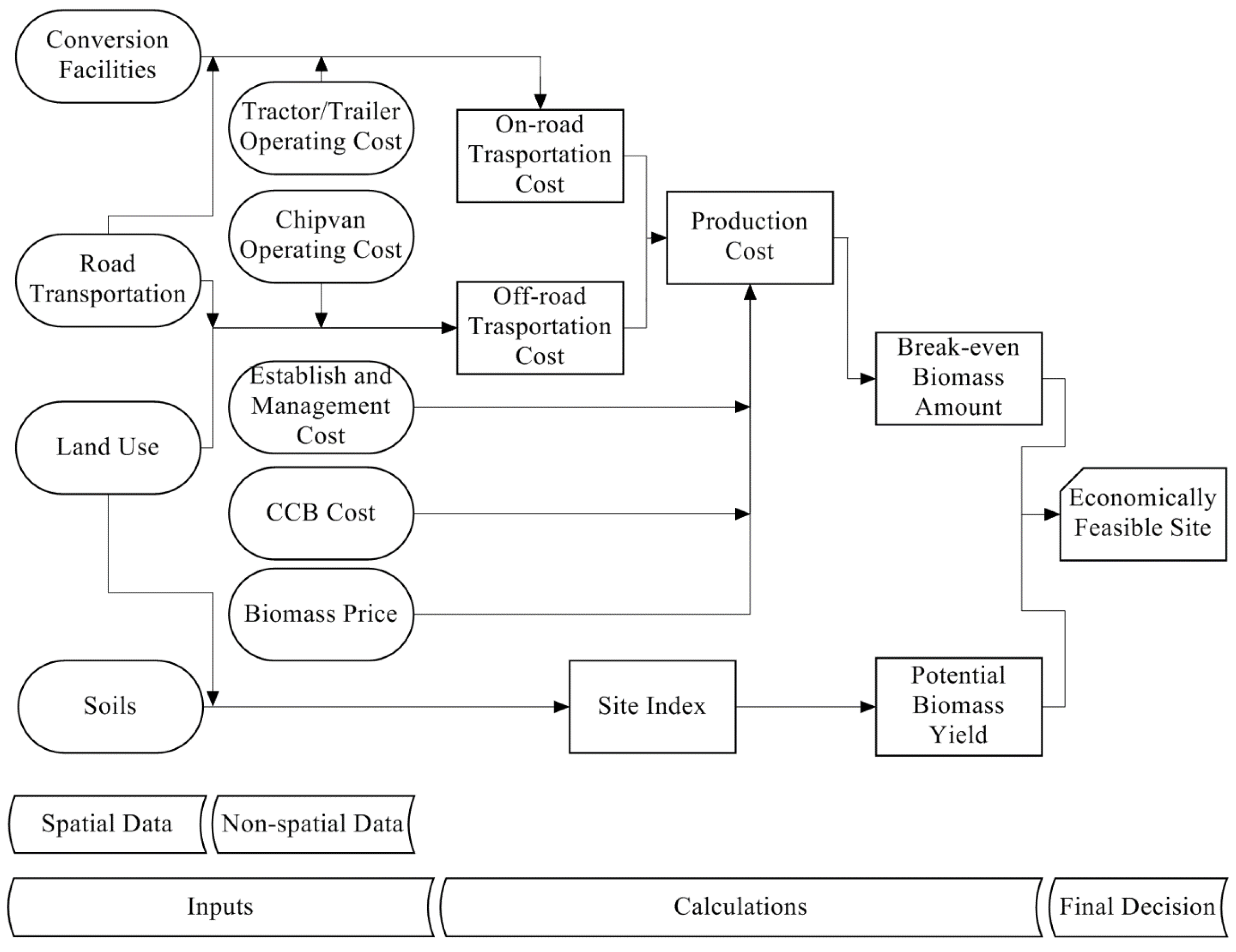
2.1. Model Description

We used a spatially-explicit model developed by Nepal et al. [26] to identify the amount and spatial distribution of economically feasible sites to establish energy crops. First, the model calculates total production costs (establishment and management, harvesting, and transportation) and combines them with the delivered biomass price to determine break-even biomass amount for each potential site (grid cell). It considers on-road and off-road transportation costs to take into account the location of potential sites relative to existing roads and thereafter to the nearest conversion facility. Second, break-even biomass amounts are compared with potential biomass yield, estimated from site index. Sites with potential biomass yields larger than the break-even biomass amounts are considered economically feasible for establishing energy crops and vice versa. A conceptual model illustrating the model inputs and calculations is presented in Figure 1.
Considering a 12-year rotation, establishment (site preparation and planting) and management (herbicide, pesticide, and fertilizer applications) costs of $1,198 ha−1 were used based on estimates provided by Kline and Coleman [33]. In the model, harvesting costs are divided into the cost of cutting, chipping and blowing chips (CCB cost) and off-road transportation. A CCB cost, constant across the study area, of 11.25 $·t−1 was used based on an economic analysis tool developed for willow crops in the eastern US [34]. Off-road transportation cost for a given grid cell was calculated considering a tractor with a 6-t trailer rental rate of 60 $·h−1, an average tractor speed of 6.5 km·h−1, and the Euclidian distance from the grid cell center to the closest existing road. On-road transportation cost for a give grid cell was calculating considering a 25-t chipvan operating costs of 78.5 $·h−1, and total travel time from the grid cell to the nearest conversion facility along the existing road network [36]. Lastly, a discounted annual property tax of 1% for agricultural land valued at 556.7 $·ha−1 [37], resulting in total discount tax of 49.29 $·ha−1 over the 12-year rotation was also included in the model.
Figure 1. Diagram illustrating the general structure of the spatially-explicit model to identify economically feasible site to establish bioenergy crops. (CCB cost indicates the cost of cutting, chipping, and blowing chips).
Forests 06 04168 g001
In the model, production costs (establishments and management, CCB, off- and on-road transportation), property taxes, and delivered biomass price are used to determine the break-even biomass amount ( V ) in t per year by grid cell as follows:
V   =   A t · [   C S P · ( 1     e r t )   +   C H P F   +     C T a x ] [ P     ( C o f f L t r a i l e r   +   C o n L v a n   +   C C B ) ] · e r t
where; A is the grid cell size (ha), which is 0.81 ha across the study area; t is the rotation age (12 years); C S P is a one-time site preparation and plantation cost that occurs during the first year of the first rotation ($·ha−1); C H P F is the sum of discounted costs for herbicide, pesticide and fertilizer treatments ($·ha−1); C T a x   is the sum of discounted property taxes ($·ha−1) over one rotation; P is the delivered biomass price ($·t−1); C o f f and C o n are the off- and on-road transportation cost ($); CCB is the cost of the cutting, chipping and blowing chips into the trailer ($·t−1); L t r a i l e r and L c h i p v a n are the loading capacity of the trailer (3 t) and the chipvan truck (12.5 t); and r is the real discount rate.
Potential biomass yields by grid cell were estimated based on site index (tree height in meters at age 50). Following procedures presented by Kline and Coleman [33], only areas with site index values between 22.9 and 38.1 meters are suitable for establishing sweetgum bioenergy crops, thus cells with sites index outside this range were estimated to yield no biomass. For other cells, their associated site index values were scaled to the suitable site index values and then related to the range of estimates from Kline and Coleman [33], from 3 to 9 t ha−1·year−1. Calculations of site index were based on a weighted score of four major soil factors: physical condition, moisture availability during the growing season, nutrient availability, and aeration [38]. These soil data were obtained from spatial and tabular soil data from the Soil Survey Geographic Database (SSURGO) [39]. For a more detailed description of procedures used to estimate biomass yields, please refer to Nepal et al. [26].

2.2. Baseline Scenario

For the baseline scenario, we only considered marginal agricultural lands to prevent competition with food production and avoid conversion of natural forest. These marginal lands included 47,158 ha of pasture/hay and barren land cover types in the 170,000-ha, four-county study area (Figure 2). A delivered biomass price of 40 $·t−1, based on the range of prices presented in previous research work [33,40,41], a real discount rate of 5%, and a property tax of 49.3 $·ha−1 were considered.
Figure 2. Distribution of pasture/hay and barren lands across the four-county study area.
Forests 06 04168 g002

2.3. Alternative Scenarios

We considered five alternative scenarios to evaluate the effects of market conditions and policy incentives on the amount and spatial distribution of sites economically feasible to establish dedicated energy crops. Scenarios I and II evaluated market conditions by applying a sensitivity analysis to examine the effect of small changes in discount rate and biomass prices, respectively. Policy incentives consisted scenarios III-V: property tax exemption, a sensitivity analysis with the inclusion of different carbon offset payments, and the inclusion of farmland as suitable sites.

2.3.1. Scenario I—Discount Rates

Although rotations of energy crops are relatively short, discount rates can still have an important influence on profitability levels and thus on the area economically feasible to establish these crops. Moreover, it is difficult to select a discount rate that can appropriately represent the dynamic nature of market conditions and the alternative options of individual investors. Other biomass studies have used a discount rate of 5% for forest valuations in the US [42,43]. We considered five real discount rates values ranging from 3 to 7 percent.

2.3.2. Scenario II—Biomass Prices

Previous studies have used a wide range of delivered biomass prices depending on species and geographic locations (i.e., [14,33,44,45,46]). We considered five biomass price values ranging from 35 to 55 $·t−1 increasing every 5 $.

2.3.3. Scenario III—Tax Incentives

Several US states offer property tax exemptions over lands used for power generation from renewable sources [47]. Although such policies for growing biomass crops are not available in Kentucky, they could prove as an effective mechanism to encourage landowners to grow these crops. We then simulated a policy scenario consisting of eliminating property taxes, by removing it from the break-even biomass calculation (Equation (1)).

2.3.4. Scenario IV—Carbon Offset Payments

Programs establishing carbon offset payments are likely to be efficient mechanisms for capturing the value of carbon sequestration, promoting the biomass utilization for energy generation, and increase landowners’ willingness to grow dedicated energy crops [46,48]. Carbon payments vary widely from 0.05 $·t−1 [49] to 15 $·t−1 [50]. Based on these exiting carbon payment values and preliminary model results, we considered four carbon payments values ranging from 1 to 4 $·t−1.
We adjusted the calculation of break-even biomass amount to include: (i) carbon offset payments incurred at the end of each rotation, which represents carbon emissions avoided by replacing coal with biomass feedstock for energy generation; and (ii) an annual carbon offset payment representing the carbon stored in biomass. The calculation of break-even biomass amount by grid cell is as follows:
V = A t [ C S P · ( 1 e r t ) + C H P F + C T a x ] [ { ( P + P c · 1.01 ) ( C o f f L t r a i l e r + C o n L v a n + C C B ) } · e r T   ] + [ 0 t P c · 1.835 e r t ]
where the additional variable P c is the carbon offset payment ($·t−1). The constant 1.835 is a conversion factor to estimate the amount of CO2 equivalent in one ton of biomass. It was determined by using the standard 0.5 converting factor from biomass to carbon content and the 3.67 factor that indicates CO2 to C atomic mass ratio [51,52,53]. The constant 1.01 multiplying P c represents the carbon emissions avoided by using one ton of biomass for electricity generation. It was determined by calculating the total electricity generated from biomass, following procedures outlined in Shrestha et al. [54], and then multiplying it by the GHG intensity of electricity generated from coal, which was 0.001236 ton CO2e per k·Wh−1 [55].

2.3.5. Scenario V—Inclusion of Agricultural Lands

Bioenergy production has been confined to marginal agricultural land, but including more productive lands might be necessary to satisfy the increasing demand of energy generation. In this analysis, we included existing row crop agricultural lands covering an additional area of about 4014 ha as potential sites for establishing bioenergy crops. The break-even biomass amount for each grid cell for this existing row crop agricultural land was also calculated using Equation (1), but including a total discount property tax of 98.49 $·ha−1, obtained from the Kentucky Department of Revenue.

3. Results

3.1. Baseline Scenario

In the spatially-explicit model there are location-independent ( C S P , C H P F , C t a x , and C C B ) and location-dependent ( C o n and C o f f ) costs. As aforementioned, location-independent costs amounted to 1198 $·ha−1) plus 11.25 $·t−1) of biomass harvested. C o f f ranged from 0 to 7.83 $·t−1) depending on proximity to existing roads with an average of 1.26 $·t−1), and C o n ranged from 0.1 to 4.76 $·t−1 with an average of 1.95 $·t−1, depending on proximity to conversion facilities. Total transportation costs varied between 0.1 and 10.98 $ t−1 with an average of 3.21 $·t−1. Break-even biomass amounts obtained by combining all production costs with the delivered biomass price of 40 $·t−1 ranged from 3.70 to 5.98 t·year−1 across the study area.
Site index values varied between 18.6 to 28.9 meters across the study area, but as suggested by Baker and Broadfoot [38], only grid cells with site index value larger than 22.9 meters were considered suitable for growing sweetgum. Out of the 47,158 ha of existing pasture/hay and barren lands, there were 17,274 ha suitable for growing sweetgum energy crops, and potential biomass yields on these sites varied between 3.24 and 4.54 t·year−1. When break-even biomass amounts were compared with biomass yield estimates by grid cell, only a total of 942 ha were identified as economically feasible to establish sweetgum, which represent about 5.5% of the total pasture/hay and barren lands. These economically feasible sites are mostly scattered throughout the study area with relatively the same amount in each county.

3.2. Alternative Scenarios

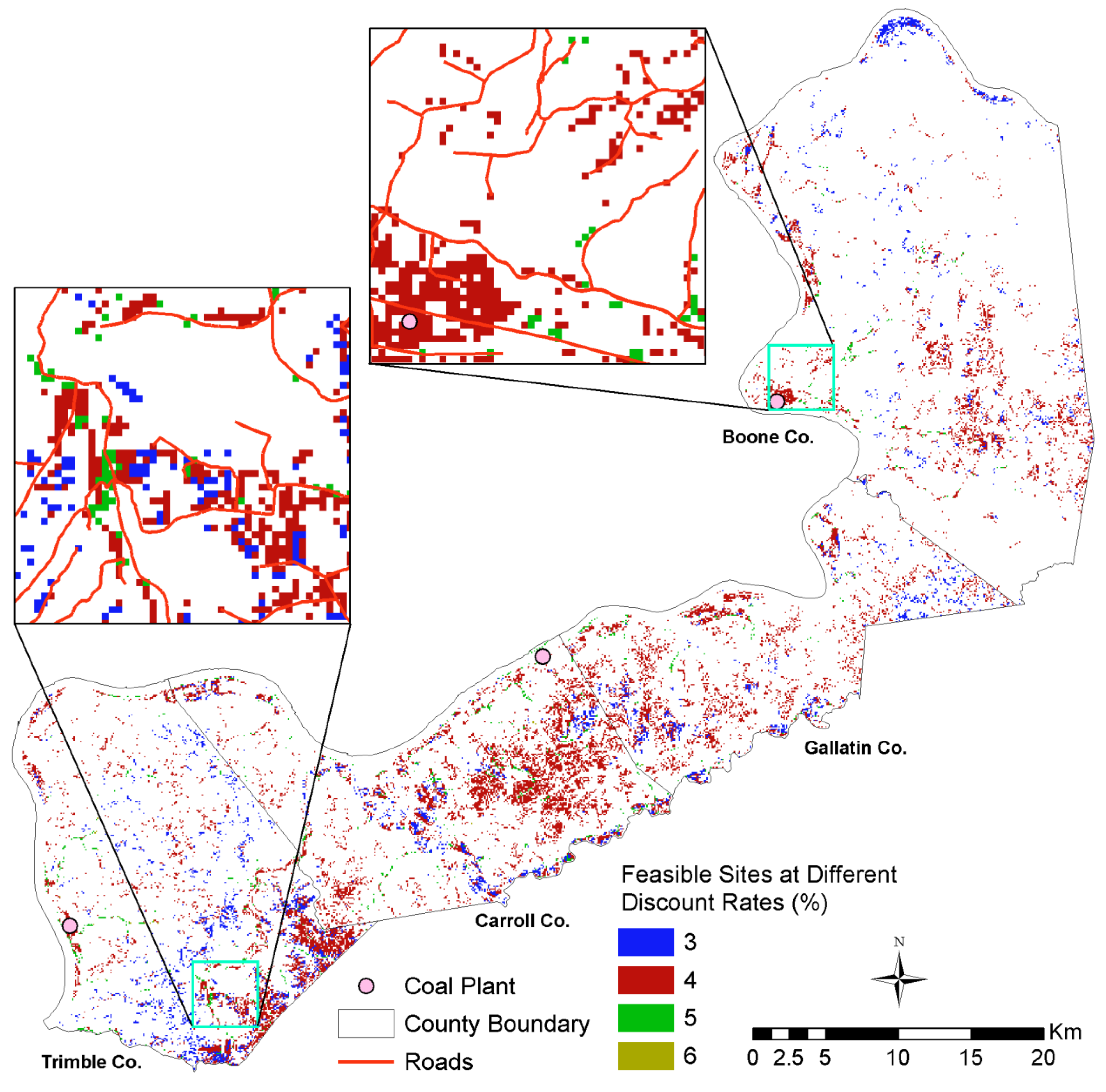
3.2.1. Scenario I—Discount Rates

Discount rate had a significant effect on the amount of area economically feasible to establish sweetgum energy crops. Increasing discount rates resulted in higher break-even biomass amounts due to the higher associated production costs (Table 1). Ranges of break-even biomass amounts overlapped and their width steadily increased with larger discount rates indicating more variability across the study area (Figure 3). Larger break-even biomass amounts with increasing discount rates caused the area economically feasible to decrease sharply from the 17,269 ha for 3% discount rate to zero ha for 7% discount rate (Table 1). When the discount rate was reduced only one percent from the baseline scenario (from 5% to 4%), the total economically feasible area increased over 14 fold from 942 ha to 13,397 ha. On the other hand, increasing the discount rate by one percent (from 5% to 6%) resulted in almost no economically feasible area.
Table 1. Scenario I results: discount rate sensitivity analysis and associated economically feasible area. (Bold font indicates baseline scenario).
Discount Rate (%)Break-Even Biomass Amount (t·year−1)Economically Feasible Area (ha)
32.6–4.317,269
43.1–5.113,397
53.7–6.0942
64.3–7.018
75.0–8.20
Figure 3. Ranges of break-even biomass amount at different discount rates.
Forests 06 04168 g003
In general, economically feasible areas considering higher discount rates (i.e., >5%) are located on sites relatively close to existing roads. As discount rate is reduced, additional areas farther from roads become economically feasible. Figure 4 shows the spatial distribution of economically feasible areas across the study area at different discount rates, where sites indicated as economically feasible for a given discount rate are also feasible for higher rates. Although for most discount rates sites are relatively scattered across the study area, some clusters can be observed in eastern Trimble Co and northeastern Carroll Co as well as along the northwestern boundary of the study area close to the Ohio River on more productive sites.
Figure 4. Spatial distribution of economically feasible sites for establishing sweetgum at different discount rates.
Forests 06 04168 g004

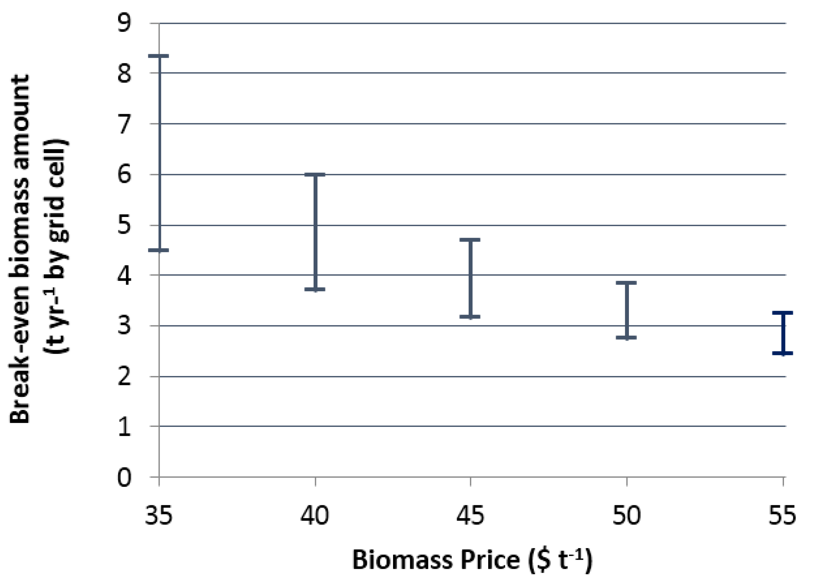
3.2.2. Scenario II—Biomass Prices

The amount of area economically feasible to establish sweetgum energy crops was also sensitive the delivered biomass price. Contrary to discount rates, increasing biomass prices resulted in reduced break-even biomass amounts because lower yields were required to cover production costs (Table 2). The reduction rate of break-even biomass amount decreased with increasing biomass price, and results suggest that break-even biomass might stabilize at around 2.5 t per year when larger values (>55 $·t−1) are considered (Figure 5). Also the variation in break-even biomass amount across the study area decreased with increasing biomass prices. Increasing biomass prices resulted in larger areas economically feasible to grow energy crops (Table 2). When the biomass price was reduced $5 from the baseline scenario (from 40 to 35 $·t−1), there was no area economically feasible. A delivered biomass price of at least 36 $·t−1 is needed to have any area feasible to grow these crops. On the other hand, increasing the delivered biomass price by $5 resulted in the total economically feasible area to increase almost fifteen fold from 942 ha to 13,903 ha. When the biomass price was further increased to 50 $·t−1, almost all suitable pasture/hay and barren land became economically feasible. When 55 $·t−1 was considered, all available area became economically feasible.
Table 2. Scenario II results: delivered biomass price sensitivity analysis and associated economically feasible area. (Bold font indicates baseline scenario).
Biomass Price ($·t−1)Break-Even Biomass Amount (t·year−1)Economically Feasible Area (ha)
354.5–8.30
403.7–6.0942
453.2–4.713,903
502.7–3.817,272
552.4–3.217,274
Figure 5. Ranges of break-even biomass amount at different biomass prices.
Forests 06 04168 g005
In general, feasible sites at lower delivered biomass prices (i.e., 40 $·t−1) were located on close proximity to existing road mostly in eastern Trimble Co and central Carroll Co and on productive site along the Ohio River (Figure 6). When higher prices were considered; sites farther away from road and on less productive areas become economically feasible; with the feasible area scattered throughout the four counties but more concentrated in eastern Trimble and Carroll counties.
Figure 6. Spatial distribution of economically feasible sites for establishing sweetgum at different delivered biomass prices.
Forests 06 04168 g006

3.2.3. Scenario III—Tax Incentives

Eliminating property taxes resulted in break-even biomass amounts about 5.5% lower (3.5–5.6 t·year−1) than the taxed scenario. When these values were compared with potential biomass yields (3.2–4.5 t·year−1) by grid cell, the total area economically feasible for sweetgum energy crops more than quadrupled from 942 ha to 4167 ha, representing about 24% of the total existing pasture/hay and barren lands. Sites that became economically feasible when property taxes were removed were located throughout the four-county study area, but relatively more concentrated in eastern Trimble and Carroll counties, and southwest Gallatin County (Figure 7).
Figure 7. Spatial distribution of economically feasible sites for establishing sweetgum with and without property tax exemptions.
Forests 06 04168 g007

3.2.4. Scenario IV—Carbon Offset Payment

Carbon offset payments had a positive effect on the amount of area economically feasible to establish sweetgum energy crops. Break-even biomass amounts decreased as carbon payments increase, although at a decreasing rate, which seemed to approach a 2–2.5 t·year−1 when larger carbon payment values (>4 $·t−1) were considered (Figure 8). The variation break-even biomass amount across the study area also decreased with increasing carbon offset payments (Table 3). Increasing carbon offset payments resulted in larger areas economically feasible because higher carbon offset payments require smaller biomass productivity to cover the production costs and provide positive economic returns. Considering only a 1 $·t−1, the economically feasible area increased by almost twelve times from 942 ha to 11,260 ha. When carbon payment was increased to 2 $·t−1, over 96% of total suitable area became economically feasible (16,615 ha). A carbon payment of 3 $·t−1 resulted in all area becoming economically feasible, and when the carbon payment was further increased, as expected all remained economically feasible. Figure 9 shows the spatial distribution of feasible areas at different carbon payments, where sites feasible at a given carbon payment are also feasible for lower values.
Figure 8. Ranges of break-even biomass amounts associated to different carbon offset payments.
Forests 06 04168 g008
Table 3. Scenario IV results: carbon offset payment sensitivity analysis and associated economically feasible area. (Bold font indicates baseline scenario).
Carbon Offset Payment ($·t−1)Break-Even Biomass Amount (t·year−1)Economically Feasible Area (ha)
03.7–6.0942
13.3–5.011,260
23.0–4.316,615
32.7–3.817,274
42.5–3.417,274
Figure 9. Spatial distribution of economically feasible sites for establishing sweetgum at different carbon offset payments.
Forests 06 04168 g009

3.2.5. Scenario V—Inclusion of Agricultural Lands

Although row crop agricultural lands are generally more productive than marginal agricultural lands, potential biomass yields were only slightly higher than pasture/hay and barren land, with averages of 3.7 vs. 3.6 t·year−1, respectively. However, larger property taxes of row crop agricultural lands compared with pasture/hay and barren lands due to their higher value, resulted in larger break-even biomass amounts ranging from 3.9 to 6.3 t·year−1. When the break-even biomass amounts were compared with potential biomass yields by grid cell within the row crop agricultural land, only 28 ha out of 4014 ha (about 0.7%) were economically feasible.

3.2.6. Combined Effects

We extended the analysis to examine the combined effects of multiple factors on the amount of economically feasible area to establish sweetgum energy crops. We considered two additional scenarios with different biomass prices and carbon offset payments with and without property taxes. For all these cases, a 5% discount rate was used.
Similar to their individual effect, increasing delivered biomass prices and carbon offset payments resulted in a rapid increase in the amount of area economically feasible to establish sweetgum energy crops (Table 4). Only the combination of lowest delivered biomass price and no carbon offset payment resulted in no area economically feasible. When carbon payments progressively increased, the amount of area economically feasible increased to 2%, 30%, 84%, and 99% of the total hay/pasture and barren lands available. Carbon payment of 3, 2, and 1 $·t−1 were required to make 100% of the area economically feasible when considering biomass prices of 40, 45, and 50 $·t−1, respectively. No carbon payment was necessary for the highest biomass price.
Table 4. Combined effects of biomass price and carbon offset payments on the amount of economically feasible area (ha) including property taxes.
Biomass Price ($·t−1)Carbon Payment ($·t−1)
01234
350279530114,48617,255
4094211,26016,61517,27417,274
4513,90617,24017,27417,27417,274
5017,27217,27417,27417,27417,274
5517,27417,27417,27417,27417,274
The same pattern of increasing amount of economically feasible area with increasing biomass price and carbon payments was observed in the scenario without property taxes (Table 5). However, more areas were economically feasible compared with scenarios including property taxes, and even the smallest biomass price with no carbon payment resulted in 46 ha being feasible. Carbon payments of 4, 3, and 1 $·t−1 were required to make all available sites economically feasible considering biomass prices 35, 40, and 45 $·t−1, respectively, and no carbon payments were required for larger biomass prices.
Table 5. Combined effects of biomass price and carbon offset payments on the amount of economically feasible area (ha) with property tax exemption.
Biomass Price ($·t−1)Carbon Payment $·t−1)
01234
354692911,59016,85017,274
40416714,28117,25417,27417,274
4516,53717,27417,27417,27417,274
5017,27417,27417,27417,27417,274
5517,27417,27417,27417,27417,274

4. Discussion

The economically feasible area was highly sensitive to market conditions expressed in terms of discount rates and delivered biomass prices. Discount rates had a positive effect on the break-even biomass amount, thus a negative effect on the economically feasible area. Results also showed increasing variation in the break-even biomass amounts across the study area with increasing discount rates. This might be explained by the fact that as discount rates increase, a given change in production costs that occur at the end of the rotation will have a larger impact on the financial return to the landowner. Results also showed a reduction in the break-even biomass amounts across the study area with increasing delivered biomass prices. Although having opposite effects, a small change in the discount rate resulted in a similar effect as a small change in delivered biomass price change from the baseline scenario. A 1% reduction in discount rate or a 5 $·t−1 increase in delivered biomass price from the baseline scenario caused the amount of economically feasible area increased from about 5% to almost 80% of the available land base. Further reducing the discount rate to 3% and increasing the delivered biomass price to 50 $·t−1 resulted in all suitable land base becoming economically feasible. Quantifying the effect of market conditions on the economically feasible area is essential to identify minimum conditions required to positively affect landowners’ willingness to grow these crops and increase biomass production by making it more competitive with alternative sources [13,54].
A policy scenario where property taxes are exempted proved as an effective mechanism to promote bioenergy production by increasing the economically feasible area over four times. It has been reported that landowners prefer tax incentive policies over direct subsidies [16]. However, to some extent, local governments depend on property taxes and eliminating them might limit their ability to support rural communities.
Incorporating policies that allow existing row crop agricultural lands as potential sites for energy crops showed only a marginal effect. Although row crop agricultural lands usually have higher site qualities, soil properties were relatively similar over both land types of agricultural lands as delineated on our land use input data, and the slightly larger biomass productivity on row crop agricultural lands did not offset the larger associated property taxes. This result indicates that there may not need to be a policy protection to restrict biomass production on agricultural lands.
On the other hand, policy scenarios installing carbon offset payments can serve as an effective mechanism to promote biomass production. Similar to delivered biomass prices, the economically feasible area was also highly sensitive to carbon payments. A carbon payment of 2 $·t−1 resulted in over 96% of the suitable land base to become economically feasible. This is important because carbon offset payments present an alternative financial venture available to landowners simply responding to favorable market incentives [56]. Moreover, in states like Kentucky where coal is the largest source of energy production, delivered coal prices remain fairly low [57]. Thus, instead of raising the delivered biomass price, installing carbon payments might be a more viable option. Installing carbon offset payments assumes that generating power from burning biomass results in greenhouse gas (GHG) savings compared with power generation from burning coal. There is still considerable debate in the literature about these potential GHG savings, mainly due to uncertainties of the many site-specific factors and productions components considered in life cycle assessments, which make difficult the accurate estimation of the amount of GHG emissions and fossil energy consumption. However, the renewable nature of biomass is recognized as a comparative advantage and had been a driving force for including carbon offset payments in policy portfolios at the state, national, and global levels [56,57,58].
Although individual factors can have a critical impact on promoting biomass for bioenergy, analyzing and modeling the overall effects of market and policies scenarios is complex. Our analysis of the interactions of biomass prices and carbon offset payments, with and without property taxes, helped examine the combined effect of these factors to identify policies that can effectively promote biomass production. As expected, in several cases, reducing the discount rate, increasing biomass prices, and introducing carbon payments resulted in all suitable land becoming economically feasible. This indicated that site productivity, and thus biomass yield, was the limiting factor. Changes in the management intensity might be an alternative to further increase areas economically suitable for the same fixed land base. For the purpose of identifying the relative effect of market and policy scenarios on the economically feasible area, we estimated biomass yields following the study of Kline and Coleman [33] that assigns an average biomass yield for low, medium, and high quality sites, which we determined based on site index. As aforementioned and as recommended by Baker and Broadfoot [38], only areas with site index between 22.9 and 38.1 meters were considered suitable for growing sweetgum crops. However, lower productivity areas might still be economically feasible, especially near existing conversion facilities where transportation costs are lower. Including these lower productivity areas is then likely to increase the economically feasible area.
Estimating biomass yields based on site-specific site conditions is not trivial as detailed information about soil properties, weather, species genetic improvements, and management scenario are required. In this study, we estimated biomass yield based on site quality as measured by site index [33]. This approach accounted for neither the relationships between site index and management scenarios nor the resulting likely different establishment costs to obtain similar biomass yields. Future studies should incorporate more detailed site-specific biomass yield models as they become available to improve the accuracy of estimates as well as properly capture the interactions between site quality and management scenarios and their contribution to biomass yields. Furthermore, site index values were calculated based on soil properties obtained from the SSURGO [39], which are prone to inconsistent results at the site level due to edge-matching. However, these soils’ data were compiled with the purpose of minimizing discontinuity in map units along soil survey area boundaries, and, most importantly, the SSURGO dataset is the most comprehensive soil dataset with the finest resolution available in the US. Another potential source of error is the reclassification of the 30-m land use raster into a 90-m resolution. The original classification accuracy of the land use raster is between 85%–95% and horizontal positional accuracy of about 10 meters. We anticipate this potential reclassification-related source of error to be marginal as 90-m cell size is 0.81 ha in size and this study evaluated economically feasible areas at a much larger scale. What is more, although we considered a single species to establish dedicated energy crops, given appropriate estimates of establishment and management costs and accurate biomass yield predictions, other species can also be included in the analysis as well as including larger geographical regions.
Lastly, this study indicates where woody energy crop production would be economically feasible given existing infrastructure and market conditions. As the amount of biomass produced even from all available sites is less 75,000 t·year−1 across the four-county study area is not large enough when delivered to the three facilities, we assumed biomass demand is always available. If additional power plant facilities or road infrastructure were built, then production costs would be reduced. In addition, there are other economic and social factors besides economic feasibility that landowners typically consider when making land-use decisions such as the opportunity cost of using the land for energy crops, which was not taken into account in the analysis. In the specific area encompassed by the study, opportunity costs range from about $80 per acre on pastureland to over $500 per acre on prime agricultural land [35]. Including such costs in the analysis would likely reduce the amount of area landowners would be willing to devote to energy crops. Other studies have shown that such costs can have a substantial impact on the availability of land for bioenergy production [61,62]. Previous work has also demonstrated that fluctuations in energy markets and an uncertain policy environment can substantially influence land-use decisions by landowners [13]. Also, non-economic drivers may influence a landowner’s willingness to supply biomass for energy. For example, studies have found that factors such as the design and security of contracts [61] and the requirement for a long-term commitment of land [63] are barriers to landowners’ willingness to plant energy crops.

5. Conclusions

We used a spatially explicit model to evaluate, and most importantly, quantify the effects of market conditions and policy incentives on the amount of land economically feasible to establish sweetgum energy plantations. The economically feasible area was highly sensitive to market conditions, expressed in terms of discount rates and delivered biomass prices. As expected, increasing delivered biomass prices and reducing discount rates showed a positive effect. It was found that raising the delivered biomass price by 5 $·t−1 and lowering the discount rate 1% from the baseline scenario (40 $·t−1 and 5%, respectively) caused a similar effect on the economically feasible area, an increment from about 5% to 80% of the available land base (hay/pasture and barren lands).
Eliminating property taxes proved to be an effective policy as the amount of economically feasible area increased from 5% to 42% of the available land base. Although landowners typically prefer tax incentive policies over direct subsidies, this policy might not be preferred by local governments because it might limit their ability to support local communities. Allowing biomass production on more productive agricultural lands, such as row crop lands, resulted in a marginal increase in the area economically feasible. Introducing carbon offset payments was also an effective policy as it had a significant effect on the amount of economically feasible area. A payment of 1 $·t−1 increased the economically feasible area from 5% to 65%. In regions where energy production comes primarily from fossil fuels, such as the eastern coal fields of the United States, this policy might be a more viable than raising delivered biomass prices.
As aforementioned, dedicated energy crops have the potential to supply a stable feedstock for the bioenergy industry, but their establishment has not been implemented on a commercial scale to significantly supply increasing energy demands. It is anticipated that policy incentives, such as the renewable portfolio standard in Kentucky, will play an important role in promoting bioenergy production [64]. Results from our analysis provide an analytical approach to quantify the effect of alternative policies and identify those that can most efficiently promote bioenergy production in terms of the amount of land where dedicated energy crops can provide positive economic returns.

Author Contributions

As part of her Master of Science in Forestry, Sandhya Nepal conducted the model run, completed the sensitivity analysis and prepared the initial version of the manuscript. Marco Contreras, George Stainback and John Lhotka designed the study, selected the market and policy scenarios relevant to the study area and prepared the final version of the manuscript.

Conflicts of Interest

The authors declare no conflict of interest.

References

  1. He, L.; English, B.C.; Daniel, G.; Hodges, D.G. Woody biomass potential for energy feedstock in United States. J. For. Econ. 2014, 20, 174–191. [Google Scholar] [CrossRef]
  2. Jeffers, R.F.; Jacobson, J.J.; Searcy, E.M. Dynamic analysis of policy drivers for bioenergy commodity. Energy Policy 2013, 52, 249–263. [Google Scholar] [CrossRef]
  3. Hinchee, M.; Rottmann, W.; Mullinax, L.; Zhang, C.; Chang, S.; Cunningham, M.; Pearson, L.; Nehra, N. Short-rotation woody crops for bioenergy and biofuels applications. Vitro Cell. Dev. Biol. Plant 2009, 45, 619–629. [Google Scholar] [CrossRef] [PubMed]
  4. Blanco-Canqui, H. Energy crops and their implication on soil and environment. Agron. J. 2010, 102, 403–419. [Google Scholar] [CrossRef]
  5. Perlack, R.D.; Wright, L.L.; Turhollow, A.F.; Graham, R.L.; Stokes, B.J.; Erbach, D.C. Biomass as Feedstock for a Bioenergy and Bioproducts Industry: The Technical Feasibility of a Billion-Ton Annual Supply; Oak Ridge National Laboratory: Oak Ridge, TN, USA; US Department of Energy and US Department of Agriculture: Washington, DC, USA, 2005. Available online: http://oai.dtic.mil/oai/oai?verb=getRecord&metadataPrefix=html&identifier=ADA436753 (accessed on 2 October 2015).
  6. US Department of Energy. US Billion-Ton Update: Biomass Supply for a Bioenergy and Bioproducts Industry; Oak Ridge National Laboratory: Oak Ridge, TN, USA, 2011; p. 227. [Google Scholar]
  7. Jose, S.; Bhaskar, T. Biomass and Biofuels—Advanced Biorefineries for Sustainable Production and Distribution; CRC Press, Taylor & Francis Group: Boca Raton, FL, USA, 2015; p. 367. [Google Scholar]
  8. Jessup, R.W. Development and status of dedicated energy crops in the United States. Vitro Cell. Dev. Biol. Plant. 2009, 45, 282–290. [Google Scholar] [CrossRef]
  9. Tyndall, J.C.; Shulte, L.A.; Hall, R.B. Expanding the US cornbelt biomass portfolio: Forester perceptions of the potential for woody biomass. Small-Scale For. 2011, 10, 287–303. [Google Scholar] [CrossRef]
  10. Leitch, Z.J.; Lhotka, J.M.; Stainback, G.A.; Stringer, J.W. Private landowner intent to supply woody feedstock for bioenergy production. Biomass Bioenergy 2013, 56, 127–136. [Google Scholar] [CrossRef]
  11. Tyner, W.E.; Taheripour, F. Advanced biofuels: Economic uncertainties, policy options, and land use impacts. Plants Bioenergy 2013, 4, 35–48. [Google Scholar]
  12. Environmental Protection Agency & National Renewable Energy Laboratory. State Bioenergy primer: Information and Resource for States on Issues, Opportunities and Options for Advancing Bioenergy. Available online: http://www.epa.gov/statelocalclimate/documents/pdf/bioenergy.pdf (accessed on 15 July 2015).
  13. Hallmann, F.W.; Amacher, G.S. Forest bioenergy adoption for a risk-averse landowener under uncertain merging biomass market. Nat. Resour. Model. 2012, 25, 482–510. [Google Scholar] [CrossRef]
  14. Chamberlain, J.F.; Miller, S.A. Policy incentives for switchgrass production using valuation of non-market ecosystem services. Energy Policy 2012, 48, 526–536. [Google Scholar] [CrossRef]
  15. Luo, Y.; Miller, S. A game theory analysis of market incentives for US switchgrass ethanol. Ecol. Econ. 2013, 93, 42–56. [Google Scholar] [CrossRef]
  16. Shivan, G.C.; Mehmood, S.R. Factors influencing nonindustrial private forest landowners’ policy preference for promoting bioenergy. For. Policy Econ. 2010, 12, 581–588. [Google Scholar] [CrossRef]
  17. Alexander, P.; Moran, D.; Smith, P.; Hastings, A.; Wang, S.; Sünnenberg, G.; Lovett, A.; Tallis, M.J.; Casella, E.; Taylor, G.; et al. Estimating UK perennial energy crop supply using farm scale models with spatially disaggregated data. Glob. Chang. Biol. Bioenergy 2014, 6, 142–155. [Google Scholar] [CrossRef] [Green Version]
  18. Alexander, P.; Moran, D.; Rounsevell, M.D.A. Evaluating potential policies for the UK perennial energy crop market to achieve carbon abatement and deliver a source of low carbon electricity. Biomass Bioenergy 2015. [Google Scholar] [CrossRef]
  19. Rizzo, D.; Martin, L.; Wohlfahrt, J. Miscanthus spatial location as seen by farmers: A machine learning approach to model real criteria. Biomass Bioenergy 2014, 66, 348–363. [Google Scholar] [CrossRef]
  20. Elobeid, A.; Tokgoz, S.; Dodder, R.; Johnson, T.; Kaplan, O.; Kurkalova, L.; Secchi, S. Integration of agricultural and energy system models for biofuel assessment. Environ. Model. Softw. 2013, 48, 1–16. [Google Scholar] [CrossRef]
  21. Egbendewe-Mondzozo, A.; Swinton, S.M.; Izaurralde, R.; Manowitz, D.H.; Zhang, X. Biomass Supply from Alternative Cellulosic Crops and Crop Residues: A Preliminary Spatial Bioeconomic Modeling Approach; Staff Paper; Department of Agricultural, Food, and Resource Economics: Washington, DC, USA; Michigan State University: East Lansing, MI, USA, 2010. Available online: http://ageconsearch.umn.edu/bitstream/98277/1/StaffPaper2010–07.pdf (accessed on 2 October 2015).
  22. Khanna, M.; Dhungana, B.; Clifton-Brown, J. Costs of producing miscanthus and switchgrass for bioenergy in Illinois. Biomass Bioenergy 2008, 32, 482–493. [Google Scholar] [CrossRef]
  23. Zubaryeva, A.; Zaccarelli, N.; del Giudice, C.; Zurlini, G. Spatially explicit assessment of local biomass availability for distributed biogas production via anaerobic co-digestion—Mediterranean case study. Renew. Energy 2012, 39, 261–270. [Google Scholar] [CrossRef]
  24. Goerndt, M.E.; Aguilar, F.X.; Miles, P.; Shifley, S.; Song, N.; Stelzer, H. Regional assessment of woody biomass physical availability as an energy feedstock for combined combustion in the US northern region. J. For. 2012, 110, 138–148. [Google Scholar] [CrossRef]
  25. Calvert, K.; Mabee, W. Spatial analysis of biomass resources within a socio-ecologically heterogeneous region: Identifying opportunities for a mixed feedstock stream. ISPRS Int. J. Geo-Inf. 2014, 3, 209–232. [Google Scholar] [CrossRef]
  26. Nepal, S.; Contreras, M.; Lhotka, J.M.; Stainback, A. A spatially explicit model to identify suitable sites to establish dedicated woody energy crops. Biomass Bioenergy 2014, 71, 245–255. [Google Scholar] [CrossRef]
  27. Fowells, H.A. Silvics of Forest Trees of the United States; US Department of Agriculture, Forest Service, Agriculture Handbook 271; US Department of Agriculture, Forest Service: Washington, DC, USA, 1965; pp. 569–572.
  28. Kormanik, P.P. Sweetgum: Liquidambar Styraciflua. In Silvics of North America, Volume 2: Hardwoods; US Department of Agriculture, Forest Service, Agriculture Handbook 654; Burns, R.M., Honkala, B.H., Eds.; Department of Agriculture, Forest Service: Washington, DC, USA, 1990. [Google Scholar]
  29. Scott, D.A.; Burger, J.A.; Kaczmarek, D.J.; Kane, M.B. Growth and nutrition response of young sweetgum plantations to repeated nitrogen fertilization on two site types. Biomass Bioenergy 2004, 27, 313–325. [Google Scholar] [CrossRef]
  30. Davis, A.A.; Trettin, C.C. Sycamore and sweetgum plantation productivity on former agricultural land in South Carolina. Biomass Bioenergy 2006, 30, 769–777. [Google Scholar] [CrossRef]
  31. Kaczmarek, D.J.; Wachelka, B.C.; Wright, J.; Steele, V.; Aubrey, D.P.; Coyle, D.R.; Coleman, M.D. Development of high-yielding sweetgum (Liquidambar styraciflua L.) plantation systems for bioenergy production in the southeastern United States. In Proceedings of the 9th Biennial Short Rotation Woody Crops Operations Working Group Conference, Oak Ridge, TN, USA, 5–8 November 2012.
  32. Jetton, R.M.; Robison, D.J. Effects of Artificial Defoliation on Growth and Biomass Accumulation in Short-Rotation Sweetgum (Liquidambar styraciflua) in North Carolina. J. Insect Sci. 2014, 14, 107–121. [Google Scholar] [CrossRef] [PubMed]
  33. Kline, K.L.; Coleman, M.D. Woody energy crops in the southern United States: Two centuries of practitioner experience. Biomass Bioenergy 2010, 34, 1655–1666. [Google Scholar] [CrossRef]
  34. National Agricultural Statistics Services, US Department of Agriculture. CropScape—Cropland Data Layer. Available online: http://nassgeodata.gmu.edu/CropScape/ (accessed on 13 May 2015).
  35. Kentucky Geography Network. Kentucky Geoportal. Available online: http://kygisserver.ky.gov/geoportal/catalog/main/home.page (accessed on 13 May 2015).
  36. Abrahamson, L.P.; Volk, T.A.; Smart, L.B.; Cameron, K.D. Shrub Willow Biomass Producer’s Handbook; College of Environmental Science and Forestry, State University of New York: Syracuse, NY, USA, 2010; p. 27. [Google Scholar]
  37. Kentucky Department of Revenue. 2011–2014 Quadrennial Recommended Agricultural Assessment Guidelines. Available online: http://revenue.ky.gov/NR/rdonlyres/1F10DE44-9317-4A79-8589-7E31CDD60B8E/0/20112014_RecommendedAgGuidelineFINAL.pdf (accessed on 15 July 2015).
  38. Baker, J.B.; Broadfoot, W.M. A Practical Field Method of Site Evaluation for Commercially Important Southern Hardwoods; General Technical Report SO-26; US Department of Agriculture, Forest Service, Southern Forest Experiment Station: New Orleans, LA, USA, 1979; p. 51.
  39. Soil Survey Geographic Database. Soil Survey Staff, Natural Resources Conservation Service, US Department of Agriculture. Web Soil Survey. Available online: http://websoilsurvey.nrcs.usda.gov/ (accessed on 13 May 2015).
  40. Ortiz, D.S.; Curtright, A.E.; Samaras, C.; Litovitz, A.; Burger, N. Near-Term Opportunities for Integrating Biomass into the US; Electric Supply: Technical Considerations; The RAND Corporation: Pittsburgh, PA, USA, 2011. [Google Scholar]
  41. Khanna, M.; Chen, X.; Huang, H.; Önal, H. Supply of cellulosic biofuel feedstocks and regional production pattern. Am. J. Agric. Econ. 2011, 93, 473–480. [Google Scholar] [CrossRef]
  42. Nesbit, T.S.; Alavalapati, J.R.; Dwivedi, P.; Marinescu, M.V. Economics of ethanol production using feedstock from slash pine (Pinus elliottii) plantations in the southern United States. South. J. Appl. For. 2011, 35, 61–66. [Google Scholar]
  43. Dwivedi, P.; Robert, B.; Stainback, A.; Carter, D.R. Impact of payments for carbon sequestrated in wood products and avoided carbon emissions on the profitability of NIPF landowners in the US South. Ecol. Econ. 2012, 78, 63–69. [Google Scholar] [CrossRef]
  44. Skog, K.; Barbour, J.; Buford, M.; Dykstra, D.; Lebow, P.; Miles, P.; Perlack, B.; Stokes, B. Forest-based biomass supply curves for the United States. J. Sustain. For. 2013, 32, 14–27. [Google Scholar] [CrossRef]
  45. Jones, G.; Loeffler, D.; Butler, E.; Hummel, S.; Chung, W. The financial feasibility of delivering forest treatment residues to bioenergy facilities over a range of diesel fuel and delivered biomass prices. Biomass Bioenergy 2013, 48, 171–180. [Google Scholar] [CrossRef]
  46. White, E.M. Woody Biomass for Bioenergy and Biofuels in the United States—A Briefing Paper; General Technical Report PNW-GTR-825; US Department of Agriculture, Forest Service, Pacific Northwest Research Station: Portland, OR, USA, 2010; p. 45.
  47. Database of State Incentives for Renewables & Efficiency. Available online: http://programs.dsireusa.org/system/program (accessed on 11 March 2015).
  48. John, S.; Watson, A. Establishing a Green Energy Crop Market in the Decatur Area; Report of the Upper Sangamom Watershed Farm Power Project; The Agricultural Watershed Institute: Decatur, IL, USA, 2007; p. 93. Available online: http://www.agwatershed.org/PDFs/Biomass_Report_Aug07.pdf (accessed on 15 July 2015).
  49. Intercontinental Exchange. CCX historical price and volume. Available online: https://www.theice.com/CCXProtocols.shtml (accessed on 18 February 2015).
  50. Regional Greenhouse Gas Initiative. CO2 Allowance Sold at $3.00 at 22nd RGGI Auction. News Release December 6, 2013. Available online: http://rggi.org/docs/Auctions/22/PR120613_Auction22.pdf (accessed on 15 July 2014).
  51. US Environmental Protection Agency. Metrics for Expressing Greenhouse Emissions: Carbon Equivalents and Carbon Dioxide Equivalents; EPA420-F-05-002; US Environmental Protection Agency: Washington, DC, USA, 2005.
  52. IPCC National Greenhouse Gas Inventories Programme. Good Practice Guidance for Land Use, Land-Use Change and Forestry; Institute for Global Environmental Strategies: Kanagawa, Japan, 2003; Available online: http://www.ipcc-nggip.iges.or.jp/public/gpglulucf/gpglulucf_files/GPG_LULUCF_FULL.pdf (accessed on 18 February 2014).
  53. Myneni, R.B.; Dong, J.; Tucker, C.J.; Kaufmann, R.K.; Kauppi, P.E.; Liski, J.; Zhou, L.; Alexeyev, V.; Hughes, M.K. A large carbon sink in the woody biomass of Northern forests. Proc. Natl. Acad. Sci. 2001, 98, 14787–14789. [Google Scholar] [CrossRef] [PubMed]
  54. Shrestha, P.; Stainback, G.A.; Dwivedi, P.; Lhotka, J.M. Economic and life-cycle analysis of forest carbon sequestration and wood-based bioenergy offsets in the central hardwood region of United States. J. Sustain. For. 2015, 34, 214–232. [Google Scholar] [CrossRef]
  55. Lemoine, D.M.; Plevin, R.J.; Cohn, A.S.; Jones, A.D.; Brandt, A.R.; Vergara, S.E.; Kammen, D.M. The climate impacts of systems depend on market and regulatory policy contexts. Environ. Sci. Technol. 2010, 44, 7347–7350. [Google Scholar] [CrossRef] [PubMed]
  56. Johnson, R.; Ramseur, J.L.; Gorte, R.W.; Stubbs, M. Potential implications of a carbon offset programs to farmers and landowners. CRS Report for Congress. 2010. Available online: http://nationalaglawcenter.org/wp-content/uploads/assets/crs/R41086.pdf (accessed on 15 July 2015).
  57. Kentucky Energy and Environment Cabinet. Kentucky Coal Facts: 2013. Available online: http://energy.ky.gov/Pages/CoalFacts.aspx (accessed on 15 July 2015).
  58. Cherubini, F.; Bird, N.D.; Cowie, A.; Jungmeier, G.; Schalamadinger, B.; Woess-Gallasch, S. Energy- and greenhouse gas-based LCA of biofuel and bioenergy systems: Key issues, ranges and recommendations. Resour. Conserv. Recycl. 2009, 53, 434–447. [Google Scholar] [CrossRef]
  59. Sebastian, F.; Royo, J.; Gomez, M. Cofiring versus biomass-fired power plants: GHG (Greehouse Gases) emissions savings comparisons by means of LAC (Life Cycle Assessment) methodology. Energy 2011, 36, 2029–2037. [Google Scholar] [CrossRef]
  60. Basu, P.; Butler, J.; Leon, M.A. Biomass co-firing options on the emission reduction and electricity generation costs in coal-fired power plants. Renew. Energy 2011, 36, 282–288. [Google Scholar] [CrossRef]
  61. Sherrington, C.; Bartley, J.; Moran, D. Farm-level constraints on the domestic supply of perennial energy crops in the UK. Energy Policy 2008, 36, 2504–2512. [Google Scholar] [CrossRef]
  62. Shastri, Y.; Rodríguez, L.; Hansen, A.; Ting, K.C. Agent-based analysis of biomass feedstock production dynamics. Bioenergy Res. 2011, 4, 258–275. [Google Scholar] [CrossRef]
  63. Glithero, N.J.; Wilson, P.; Ramsden, S.J. Prospects for arable farm uptake of Short Rotation Coppice willow and miscanthus in England. Appl. Energy 2013, 107, 209–218. [Google Scholar] [CrossRef] [PubMed]
  64. Catron, J.; Stainback, G.A.; Dwivedi, P.; Lhotka, J.M. Bioenergy development in Kentucky: A SWOT-ANP analysis. For. Policy Econ. 2013, 28, 38–43. [Google Scholar] [CrossRef]

