
Wall-to-Wall Forest Mapping Based on Digital Surface Models from Image-Based Point Clouds and a NFI Forest Definition


Abstract
:1. Introduction
- (i)
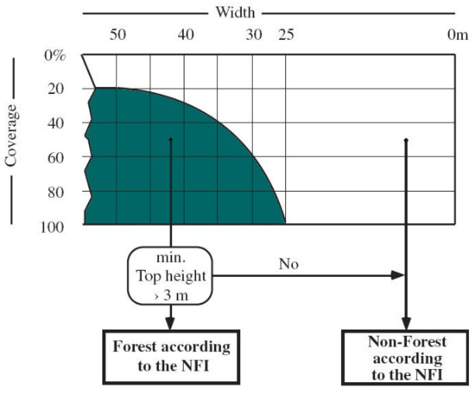
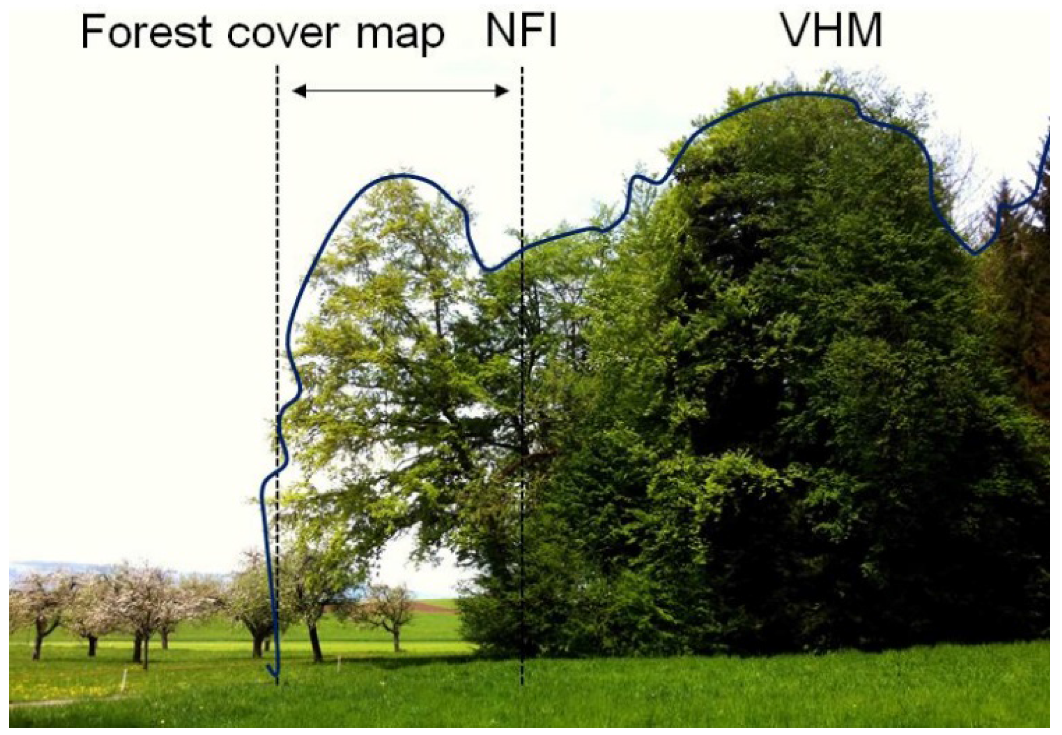
- Existing forest cover maps have often been produced with an oversimplified definition of forest, and are therefore not congruent with the respective NFI definition, which consists mostly of the key criteria: (1) minimum tree height; (2) minimum tree crown coverage; (3) minimum area and/or minimum width; and (4) land use [4].
- (ii)
- Problems arise regarding land use, which is a key parameter in NFI forest definition but hardly assessable when using remotely sensed data—in contrast to land cover which is assessable. For example, a temporary unstocked area, e.g., after impacts such as fire, storm, or harvesting will be identified as non-forest area when using remote sensing data and techniques, but will in fact maintain its status as a forest within the NFI.
- (iii)
- Unavoidable restrictions occur due to the simplified level of detail of existing forest cover maps, which results in an insufficient and inaccurate representation of forest borders, gaps, and parts with open or dense forests.
2. Material
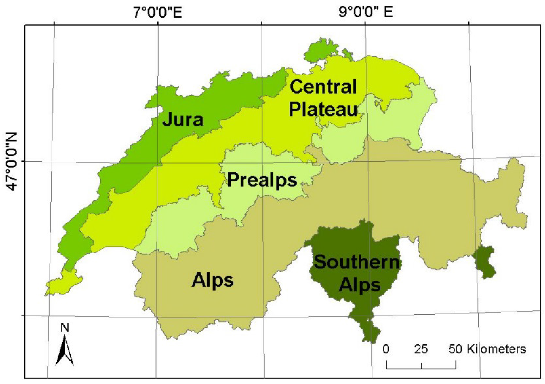
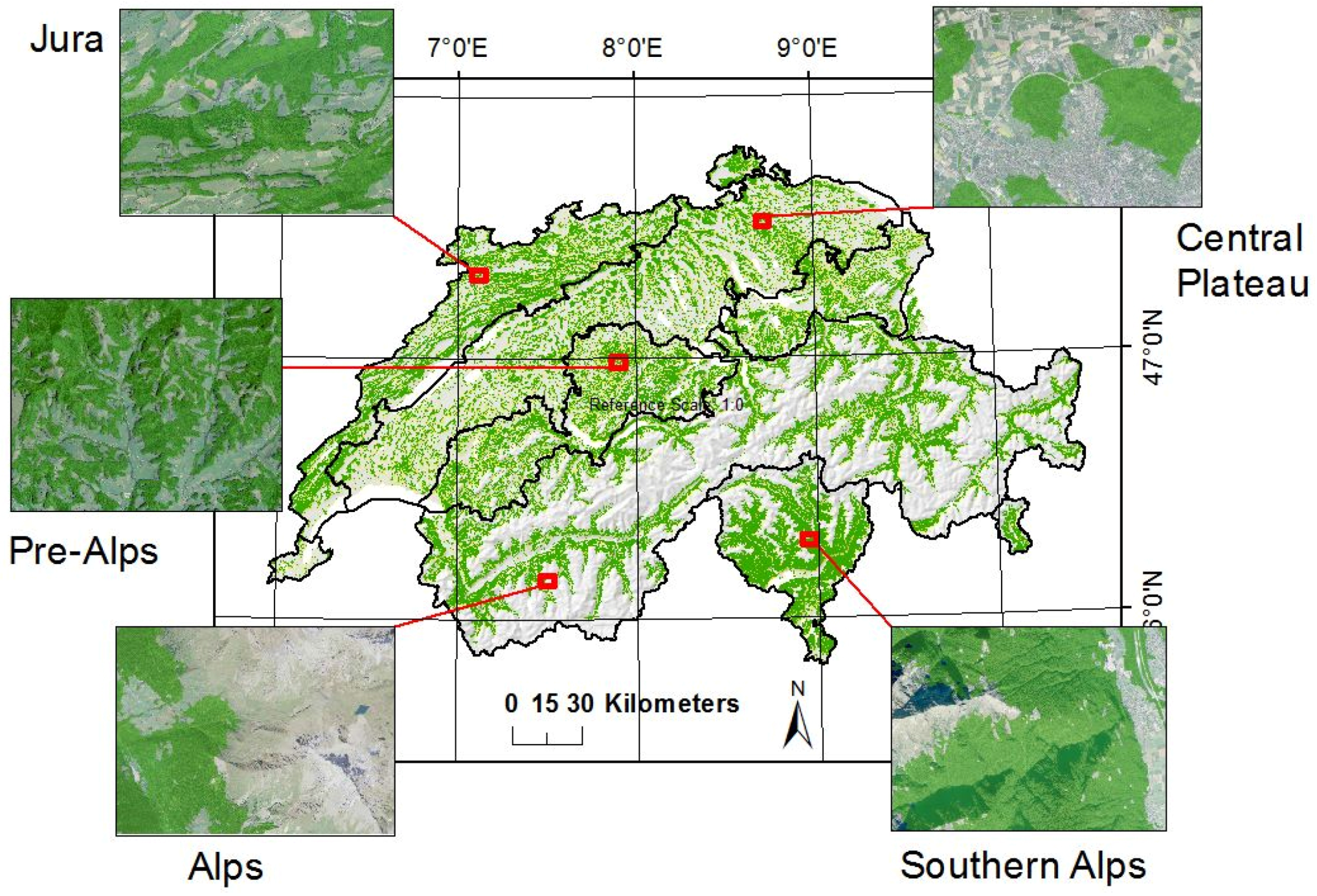
2.1. Study Area

2.2. Remote Sensing Data
2.2.1. Aerial Images

| Parameter | ADS40-SH40 | ADS40-SH52 | ADS80-SH82 |
|---|---|---|---|
| Time of operation | until 2007 | 2008–present | 2009–present |
| Sensor | Three-line CCD scanner | Three-line CCD scanner | Three-line CCD scanner |
| Dynamic range of the CCD | 12-bit | 12-bit | 12-bit |
| Spectral bands (nm) | Panchromatic 465–680 | Panchromatic 465–680 | Panchromatic 465–680 |
| Blue 430–490 | Blue 428–492 | Blue 428–492 | |
| Green 535–585 | Green 533–587 | Green 533–587 | |
| Red 610–660 | Red 608–662 | Red 608–662 | |
| Near infrared 835–885 | Near infrared 833–887 | Near infrared 833–887 | |
| CCD elements | 8 CCD lines with 12,000 pixels each | 12 CCD lines with 12,000 pixels each | 12 CCD lines with 12,000 pixels each |
| Pixel size (μm) | 6.5 | 6.5 | 6.5 |
| Bands used for matching | PAN/RGB | CIR/CIR | CIR/CIR |
2.2.2. Digital Surface Model
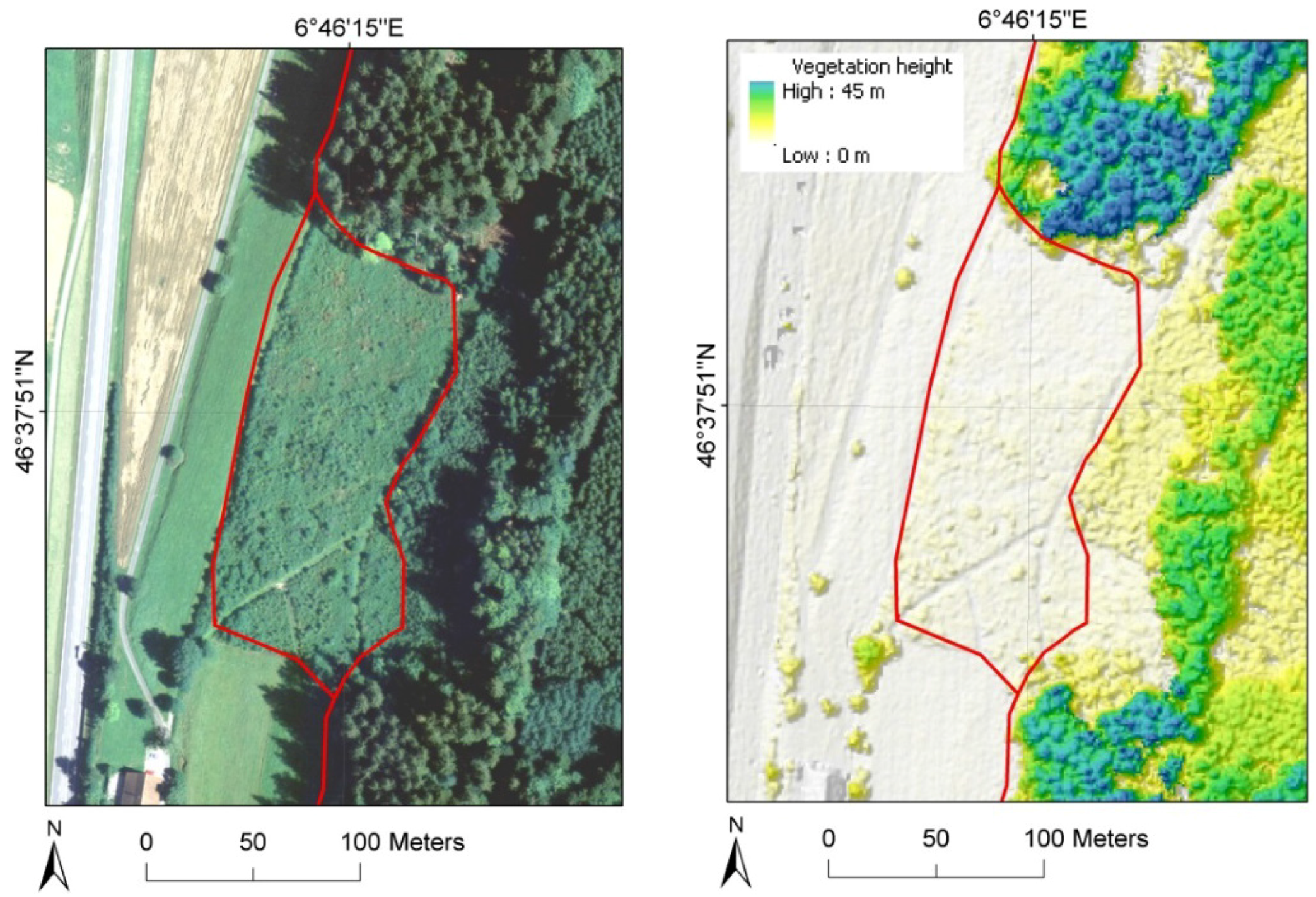
2.2.3. Vegetation Height Model
2.3. Reference Data
3. Method
3.1. Forest Definition of the Swiss National Forest Inventory

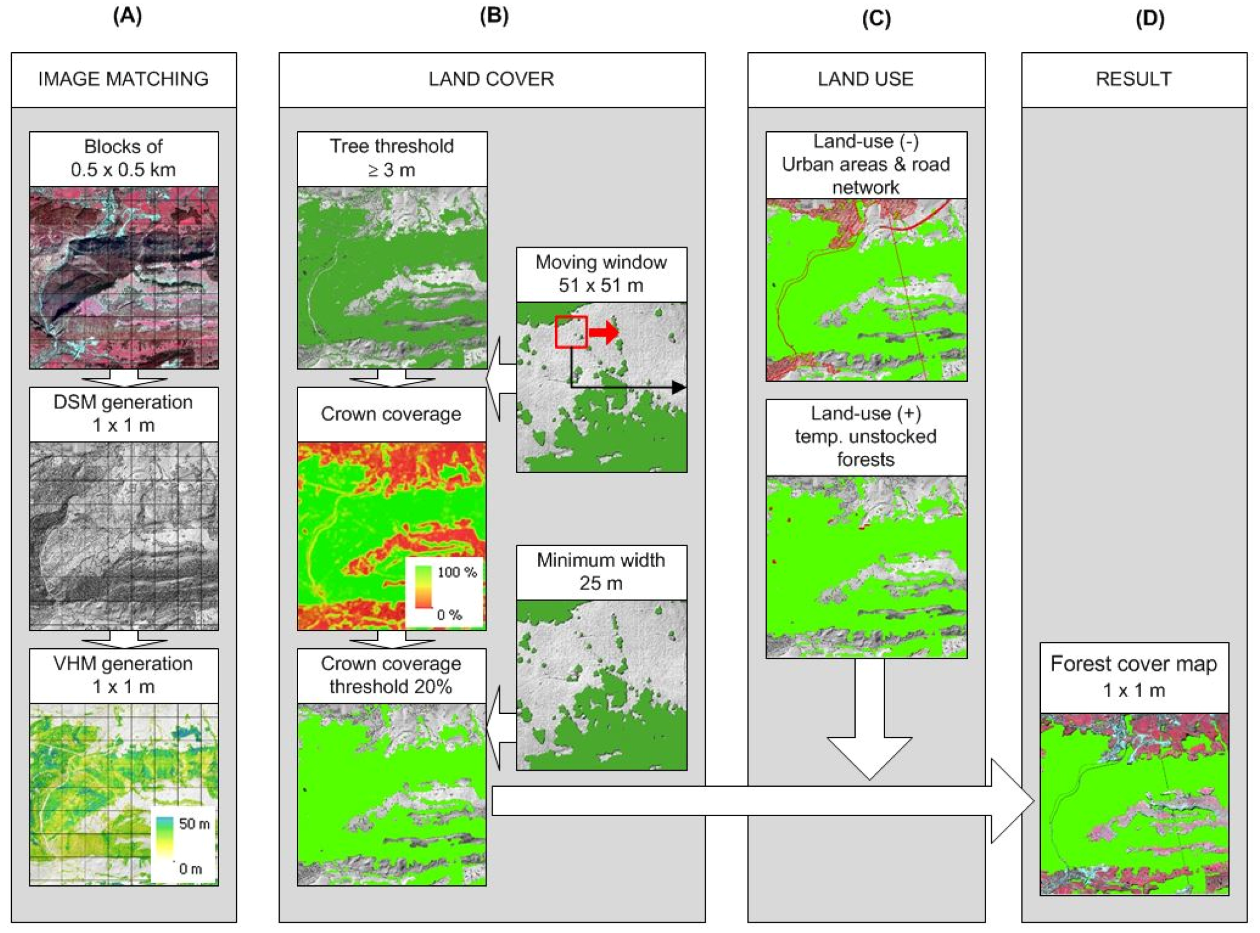
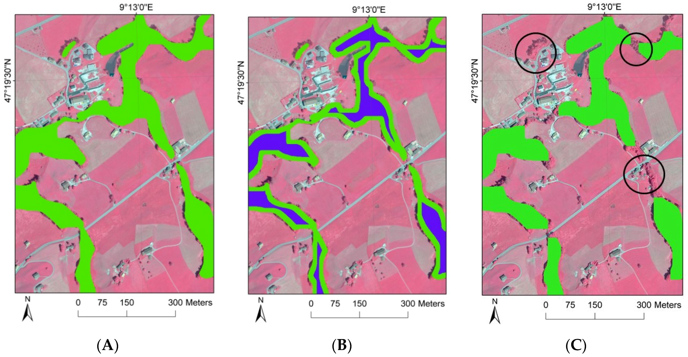
3.2. Workflow of Wall-To-Wall Forest Mapping

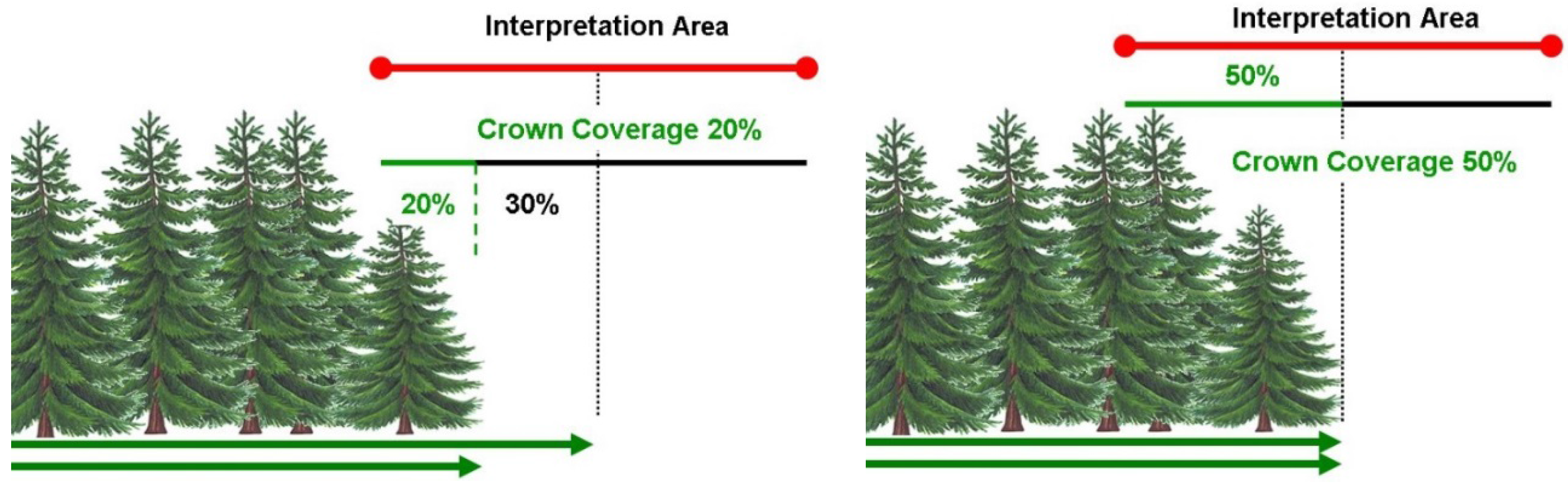
3.3. Land Cover Criteria of the Swiss NFI


3.4. Land Use Criterion

4. Results

4.1. Comparison with NFI Estimations
| Production Region | Forest Cover Map (ha) | NFI (ha) (SE%) | Difference |
|---|---|---|---|
| Jura | 214,824 | 203,669 (1) | 5.5% |
| Central Plateau | 248,285 | 233,454 (1) | 6.4% |
| Prealps | 242,026 | 227,725 (1) | 6.3% |
| Alps | 410,809 | 405,429 (1) | 1.3% |
| Southern Alps | 177,827 | 168,731 (2) | 5.4% |
| Switzerland | 1,293,771 | 1,239,008 (1) | 4.4% |
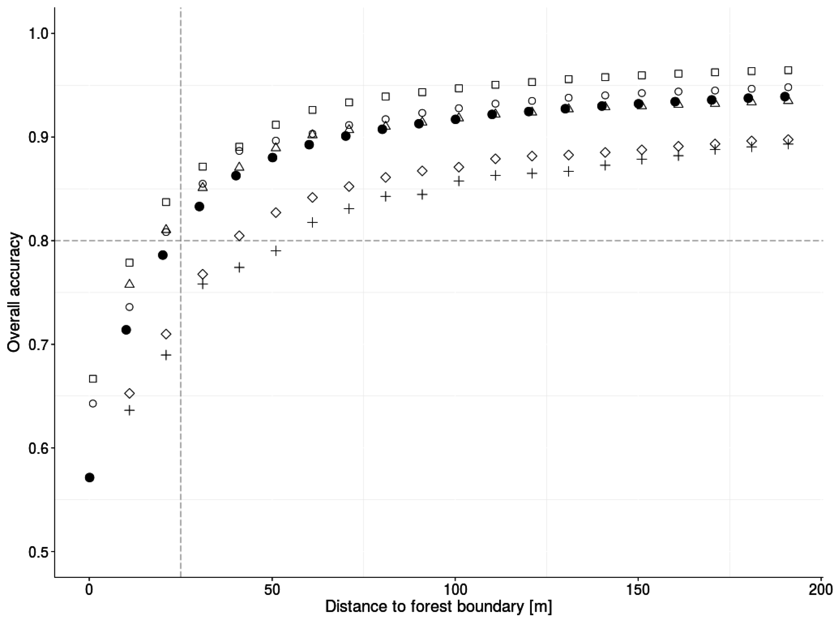
4.2. Comparison with NFI Sample Plot Data
| Validation Based on | N Plots | OA | Error of Omission (%) | Error of Commission (%) | |
|---|---|---|---|---|---|
| All plots | 9984 | 0.97 | 3.8 | 10.1 | |
| Height above sea level [m] | <600 | 2800 | 0.98 | 1.1 | 9.9 |
| 600–1000 | 2105 | 0.96 | 0.7 | 10.1 | |
| 1001–1400 | 1114 | 0.94 | 2.3 | 8.3 | |
| 1401–1800 | 878 | 0.91 | 10.2 | 10.5 | |
| >1800 | 3087 | 0.99 | 19.7 | 17.6 | |
| Deciduous | 797 | 0.98 | 1.5 | 0.8 | |
| Coniferous | 1372 | 0.96 | 4.1 | 0.3 | |
| Production region | Jura | 1307 | 0.97 | 0.4 | 7.1 |
| Central Plateau | 2471 | 0.98 | 1.7 | 7.9 | |
| Prealps | 1549 | 0.95 | 3.6 | 13.5 | |
| Alps | 4075 | 0.97 | 7.0 | 10.9 | |
| Southern Alps | 582 | 0.94 | 8.1 | 15.1 |

5. Discussion and Conclusions
5.1. General Aspects of the Mapping Approach
5.2. Constraints of the Forest Mapping Approach
5.3. Errors of Commission

5.4. Errors of Omission


5.5. Operational Use of the Forest Cover Map
5.6. Outlook and Summary
- -
- Differences between the NFI estimated forest area and the forest cover map can be further reduced by implementing the 1:1 minimum crown coverage and minimum width functions as used in the Swiss NFI.
- -
- The shrinking functions applied to the forest cover map could be adapted, for instance, by using different thresholds for deciduous and coniferous dominated forest borders.
- -
- The effect of different forest pattern on the landscape level, especially regarding forest edges for the proposed method should be further investigated as described in [45].
- -
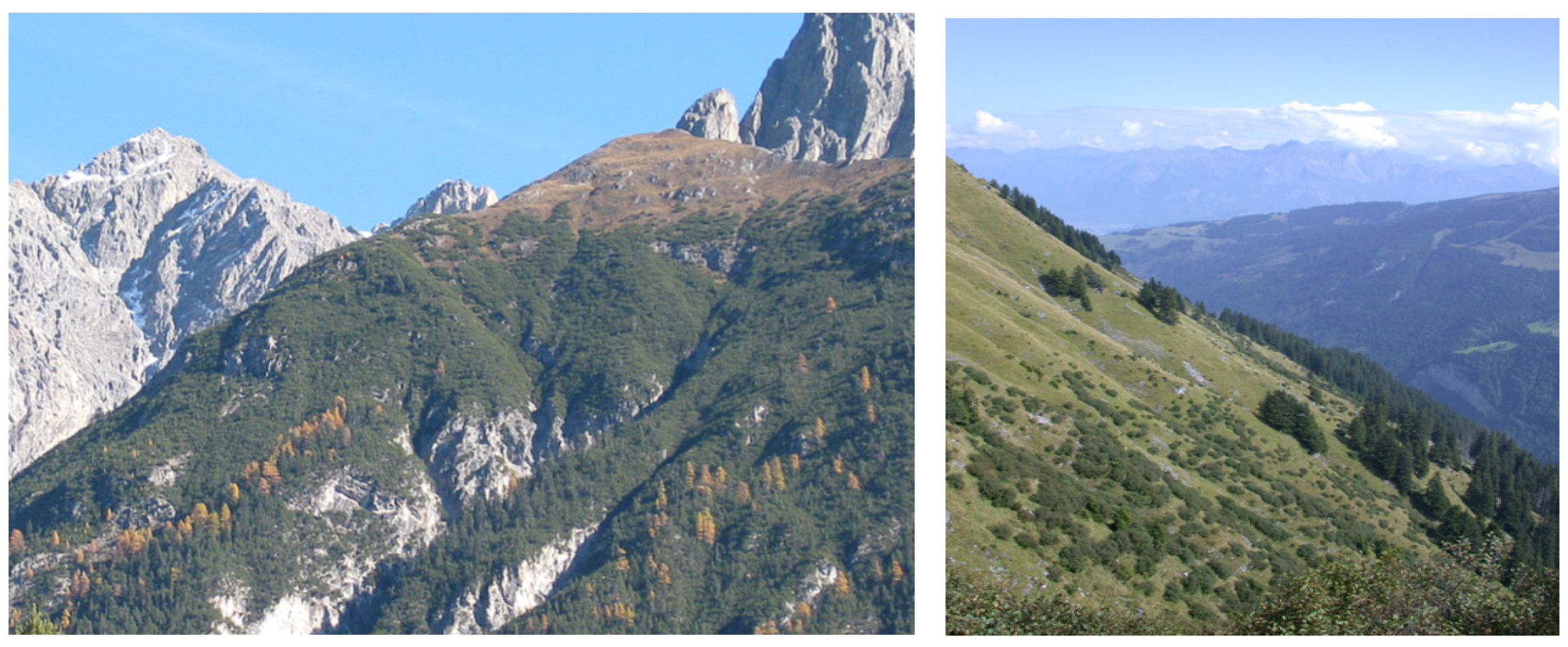
- Further research is also needed to improve the accuracy of the forest cover map at the upper tree line in the Alps. Image matching based on upcoming imagery with the same 25 cm spatial resolution that is standard for the Central Plateau in Switzerland will reduce the number of omitted narrow crowns of coniferous trees.
Acknowledgments
Author Contributions
Conflicts of Interest
References
- Food and Agriculture Organization (FAO). Global Forest Resources Assessment 2010: Main Report; FAO: Rome, Italy, 2010. [Google Scholar]
- Hansen, M.C.; Potapov, P.V.; Moore, R.; Hancher, M.; Turubanova, S.A.; Tyukavina, A.; Thau, D.; Stehman, S.V.; Goetz, S.J.; Loveland, T.R.; et al. High-resolution global maps of 21st-century forest cover change. Science 2013, 342, 850–853. [Google Scholar] [CrossRef] [PubMed]
- Lawrence, M.; McRoberts, R.E.; Tomppo, E.; Thomas, G.; Karl, G. Comparisons of National Forest Inventories. In National Forest Inventories—Pathways for Common Reporting; Tomppo, E., Gschwantner, T., Lawrence, M., McRoberts, R.E., Eds.; Springer Science and Business Media B.V.: Berlin, Germany, 2010; pp. 19–32. [Google Scholar]
- Tomppo, E.; Gschwantner, T.; Lawrence, M.; McRoberts, R.E. National Forest Inventories-Pathways for Common Reporting; Springer Science and Business Media B.V.: Berlin, Germany, 2010; p. 612. [Google Scholar]
- Koch, B.; Dees, M.; van Brusselen, J.; Eriksson, L.; Fransson, J.; Gallaun, H.; Leblon, B.; McRoberts, R.E.; Nilsson, M.; Schardt, M.; et al. Forestry applications. In Advances in Photogrammetry, Remote Sensing and Spatial Information—ISPRS 2008 Congress Book; Li, Z., Chen, J., Baltsavias, E., Eds.; Taylor & Francis Group: London, UK, 2008; pp. 439–468. [Google Scholar]
- Barrett, F.; McRoberts, R.E.; Tomppo, E.; Cienciala, E.; Waser, L.T. A questionnaire-based review of the operational use of remotely sensed data by national forest inventories. Remote Sens. Environ. 2016, in press. [Google Scholar]
- Kleinn, C.; Ramírez, C.; Holmgren, P.; Lobo, S.; Chavez, G. A national forest resources assessment for Costa Rica based on low intensity sampling. For. Ecol. Manag. 2005, 210, 9–23. [Google Scholar] [CrossRef]
- Maltamo, M.; Naesset, E.; Vauhkonen, J. Forestry applications of airborne laser scanning: Concepts and case studies. In Managing Forest Ecosystems 27; Springer Science and Business Media: Dodrecht, The Netherlands, 2014; p. 464. [Google Scholar]
- McRoberts, R.E.; Liknes, G.C.; Domke, G.M. Using a remote sensing-based, percent tree cover map to enhance forest inventory estimation. For. Ecol. Manag. 2014, 331, 12–18. [Google Scholar] [CrossRef]
- McRoberts, R.E.; Tomppo, E.O. Remote sensing support for national forest inventories. Remote Sens. Environ. 2007, 110, 412–419. [Google Scholar] [CrossRef]
- Tomppo, E.; Haakana, M.; Katila, M.; Peräsaari, J. Multi-source national forest inventory-methods and applications. In Managing Forest Ecosystems 18; Springer Science and Business Media B.V.: Berlin, Germany, 2008. [Google Scholar]
- Tomppo, E.; Halme, M. Using coarse scale forest variables as ancillary information and weighting of variables in k-NN estimation: A genetic algorithm approach. Remote Sens. Environ. 2004, 92, 1–20. [Google Scholar] [CrossRef]
- Food and Agriculture Organization (FAO). Global Forest Land-Use Change 1990–2005; FAO: Rome, Italy, 2012. [Google Scholar]
- The Global Forest Watch. Available online: http://www.globalforestwatch.org/map/3/15.00/27.00/ALL/grayscale/loss,forestgain?begin=2001-01-01&end=2015-01-01&threshold=30 (accessed on 5 November 2015).
- Bartholomé, E.; Belward, A.S. GLC2000: A new approach to global land cover mapping from Earth observation data. Int. J. Remote Sens. 2005, 26, 1959–1977. [Google Scholar] [CrossRef]
- World’s First High-Resolution Global Forest/Non-Forest Map. Available online: http://global.jaxa.jp/article/special/geo/shimada_e.html (accessed on 5 November 2015).
- European Joint Research Center JRC. Forest Cover Map—2006. Available online: http://forest.jrc.ec.europa.eu/activities/forest-mapping/forest-cover-map-2006/ (accessed on 5 November 2015).
- Waser, L.T.; Baltsavias, E.; Ecker, K.; Eisenbeiss, H.; Feldmeyer-Christe, E.; Ginzler, C.; Küchler, M.; Zhang, L. Assessing changes of forest area and shrub encroachment in a mire ecosystem using digital surface models and aerial images. Remote Sens. Environ. 2008, 112, 1956–1968. [Google Scholar] [CrossRef]
- Wang, Z.; Ginzler, C.; Waser, L.T. A novel method to assess short-term forest cover changes based on digital surface models from image-based point clouds. Forestry 2015, 88, 429–440. [Google Scholar] [CrossRef]
- Magdon, P.; Fischer, C.; Fuchs, H.; Kleinn, C. Translating criteria of international forest definitions into remote sensing image analysis. Remote Sens. Environ. 2014, 149, 252–262. [Google Scholar] [CrossRef]
- Eriksson, L.E.B.; Santoro, M.; Wiesmann, A.; Schmullius, C.C. Multitemporal JERS repeat-pass coherence for growing-stock volume estimation of siberian forest. IEEE Trans. Geosci. Remote Sens. 2003, 41, 1561–1570. [Google Scholar] [CrossRef]
- Gebhardt, S.; Wehrmann, T.; Ruiz, M.; Maeda, P.; Bishop, J.; Schramm, M.; Kopeinig, R.; Cartus, O.; Kellndorfer, J.; Ressl, R.; et al. MAD-MEX: Automatic wall-to-wall land cover monitoring for the Mexican REDD-MRV program using all Landsat data. Remote Sens. 2014, 6, 3923–3943. [Google Scholar] [CrossRef]
- Schepaschenko, D.; See, L.; Lesiv, M.; McCallum, I.; Fritz, S.; Salk, C.; Moltchanova, E.; Perger, C.; Shchepashchenko, M.; Shvidenko, A.; et al. Development of a global hybrid forest mask through the synergy of remote sensing, crowdsourcing and fao statistics. Remote Sens. Environ. 2015, 162, 208–220. [Google Scholar] [CrossRef]
- Shimada, M.; Itoh, T.; Motooka, T.; Watanabe, M.; Shiraishi, T.; Thapa, R.; Lucas, R. New global forest/non-forest maps from ALOS PALSAR data (2007–2010). Remote Sens. Environ. 2014, 155, 13–31. [Google Scholar] [CrossRef]
- Mustonen, J.; Packalén, P.; Kangas, A. Automatic segmentation of forest stands using a canopy height model and aerial photography. Scand. J. For. Res. 2008, 23, 534–545. [Google Scholar] [CrossRef]
- Straub, C.; Weinacker, H.; Koch, B. A fully automated procedure for delineation and classification of forest and non-forest vegetation based on full waveform laser scanner data. Int. Arch. Photogramm. Remote Sens. Spat. Inf. Sci. 2008, 37, 1013–1019. [Google Scholar]
- Eysn, L.; Hollaus, M.; Schadauer, K.; Pfeifer, N. Forest delineation based on airborne lidar data. Remote Sens. 2012, 4, 762–783. [Google Scholar] [CrossRef]
- White, J.C.; Wulder, M.A.; Vastaranta, M.; Coops, N.C.; Pitt, D.; Woods, M. The utility of image-based point clouds for forest inventory: A comparison with airborne laser scanning. Forests 2013, 4, 518–536. [Google Scholar] [CrossRef]
- Waser, L.T.; Baltsavias, E.; Ecker, K.; Eisenbeiss, H.; Ginzler, C.; Küchler, M.; Thee, P.; Zhang, L. High-resolution digital surface models (DSMs) for modelling fractional shrub/tree cover in a mire environment. Int. J. Remote Sens. 2008, 29, 1261–1276. [Google Scholar] [CrossRef]
- Wang, Z.; Boesch, R. Color-and texture-based image segmentation for improved forest delineation. IEEE Trans. Geosci. Remote Sens. 2007, 45, 3055–3062. [Google Scholar] [CrossRef]
- Debella-Gilo, M.; Bjørkelo, K.; Breidenbach, J.; Rahlf, J. Object-based analysis of aerial photogrammetric point cloud and spectral data for land cover mapping. Int. Arch. Photogramm. Remote Sens. Spat. Inf. Sci. 2013, XL-1/W1, 63–67. [Google Scholar]
- Reese, H.; Nordkvist, K.; Nyström, M.; Bohlin, J.; Olsson, H. Combining point clouds from image matching with SPOT 5 multispectral data for mountain vegetation classification. Int. J. Remote Sens. 2015, 36, 403–416. [Google Scholar] [CrossRef]
- The topographic landscape model TML. Available online: http://www.swisstopo.admin.ch/internet/swisstopo/en/home/topics/geodata/tlm.html (accessed on 6 November 2015).
- Abegg, M.; Brändli, U.-B.; Cioldi, F.; Fischer, C.; Herold-Bonardi, A.; Huber, M.; Keller, M.; Meile, R.; Rösler, E.; Speich, S.; et al. Fourth National Forest Inventory—Result Tables and Maps on the Internet for the NFI 2009–2013 (NFI4b); Swiss Federal Institute for Forest, Snow and Landscape Research WSL: Birmensdorf, Switzerland, 2014. [Google Scholar]
- Brändli, U.-B. Swiss National Forest Inventory. Results of the Third Assessment 2004–2006; Swiss Federal Institute for Forest, Snow and Landscape Research WSL: Birmensdorf, Switzerland, 2010; p. 312. [Google Scholar]
- Waser, L.T. Airborne Remote Sensing Data for Semi-Automated Extraction of Tree Area and Classification of Tree Species. Ph.D. Thesis, ETH Zurich, Zurich, Switzerland, 2012. [Google Scholar]
- Ginzler, C.; Hobi, M. Countrywide stereo-image matching for updating digital surface models in the framework of the Swiss national forest inventory. Remote Sens. 2015, 7, 4343–4370. [Google Scholar] [CrossRef]
- Keller, M. Swiss National Forest Inventory. Manual for Terrestrial Survey; Swiss Federal Institute for Forest, Snow and Landscape Research WSL: Birmensdorf, Switzerland, 2013; p. 214. [Google Scholar]
- R Core teAm. The R Manuals. Available online: http://cran.r-project.org/manuals.html (accessed on 16 September 2015).
- Lund, H.G. Definitions of Forest, Deforestation, Afforestation, and Reforestation. Available online: https://www.researchgate.net/publication/259821294_Definitions_of_Forest_Deforestation_Afforestation_and_Reforestation (accessed on 11 December 2015).
- Lanz, A.; Brändli, U.-B.; Brassel, P.; Ginzler, C.; Kaufmann, E.; Thrürig, E. Switzerland. National Forest Inventories—Pathways for Common Reporting; Tomppo, E., Gschwantner, T., Lawrence, M., McRoberts, R.E., Eds.; Springer Science and Business Media B.V.: Berlin, Germany, 2010; pp. 555–565. [Google Scholar]
- Brassel, P.; Lischke, H. Swiss National Forest Inventory: Methods and Models of the Second Assessment; Swiss Federal Institute for Forest, Snow and Landscape Research WSL: Birmensdorf, Switzerland, 2001. [Google Scholar]
- Mathys, L.; Ginzler, C.; Zimmermann, N.E.; Brassel, P.; Wildi, O. Sensitivity assessment on continuous landscape variables to classify a discrete forest area. For. Ecol. Manag. 2006, 229, 111–119. [Google Scholar] [CrossRef]
- Ginzler, C.; Bärtschi, H.; Bedolla, A.; Brassel, P.; Hägeli, M.; Hauser, M.; Kamphues, M.; Laranjeiro, L.; Mathys, L.; Uebersax, D.; et al. Aerial Image Interpretation LFI 3. Interpretationsanleitung zum Dritten Landesforstinventar; Swiss Federal Institute for Forest, Snow and Landscape Research WSL: Birmensdorf, Switzerland, 2005; p. 87. [Google Scholar]
- Magdon, P.; Kleinn, C. Uncertainties of forest area estimates caused by the minimum crown cover criterion—A scale issue relevant to forest cover monitoring. Environ. Monit. Assess. 2013, 185, 5345–5360. [Google Scholar] [CrossRef] [PubMed]
- Campbell, J.B.; Wynne, R.H. Introduction to Remote Sensing, 5th ed.; The Guilford Press: New York, NY, USA, 2011. [Google Scholar]
© 2015 by the authors; licensee MDPI, Basel, Switzerland. This article is an open access article distributed under the terms and conditions of the Creative Commons by Attribution (CC-BY) license (http://creativecommons.org/licenses/by/4.0/).
Share and Cite
Waser, L.T.; Fischer, C.; Wang, Z.; Ginzler, C. Wall-to-Wall Forest Mapping Based on Digital Surface Models from Image-Based Point Clouds and a NFI Forest Definition. Forests 2015, 6, 4510-4528. https://doi.org/10.3390/f6124386
Waser LT, Fischer C, Wang Z, Ginzler C. Wall-to-Wall Forest Mapping Based on Digital Surface Models from Image-Based Point Clouds and a NFI Forest Definition. Forests. 2015; 6(12):4510-4528. https://doi.org/10.3390/f6124386
Chicago/Turabian StyleWaser, Lars T., Christoph Fischer, Zuyuan Wang, and Christian Ginzler. 2015. "Wall-to-Wall Forest Mapping Based on Digital Surface Models from Image-Based Point Clouds and a NFI Forest Definition" Forests 6, no. 12: 4510-4528. https://doi.org/10.3390/f6124386