Article

A Quantitative Assessment of Forest Cover Change in the Moulouya River Watershed (Morocco) by the Integration of a Subpixel-Based and Object-Based Analysis of Landsat Data

by
Fernando J. Aguilar
1,*,
Abderrahim Nemmaoui
1,
Manuel A. Aguilar
1,
Mimoun Chourak
2,
Yassine Zarhloule
3 and
Andrés M. García Lorca
4
1
Department of Engineering, University of Almería, Ctra. de Sacramento s/n, La Cañada de San Urbano, 04120 Almería, Spain
2
National School of Applied Sciences, University of Mohamed I, Oujda 6000, Morocco
3
High School of Technology, University of Mohamed I, Oujda 6000 Morocco
4
Department of Geography, University of Almería, Ctra Sacramento s/n, La Cañada de San Urbano, 04120 Almería, Spain
*
Author to whom correspondence should be addressed.
Forests 2016, 7(1), 23; https://doi.org/10.3390/f7010023
Submission received: 5 November 2015 / Revised: 6 January 2016 / Accepted: 7 January 2016 / Published: 15 January 2016

Abstract

:
A quantitative assessment of forest cover change in the Moulouya River watershed (Morocco) was carried out by means of an innovative approach from atmospherically corrected reflectance Landsat images corresponding to 1984 (Landsat 5 Thematic Mapper) and 2013 (Landsat 8 Operational Land Imager). An object-based image analysis (OBIA) was undertaken to classify segmented objects as forested or non-forested within the 2013 Landsat orthomosaic. A Random Forest classifier was applied to a set of training data based on a features vector composed of different types of object features such as vegetation indices, mean spectral values and pixel-based fractional cover derived from probabilistic spectral mixture analysis). The very high spatial resolution image data of Google Earth 2013 were employed to train/validate the Random Forest classifier, ranking the NDVI vegetation index and the corresponding pixel-based percentages of photosynthetic vegetation and bare soil as the most statistically significant object features to extract forested and non-forested areas. Regarding classification accuracy, an overall accuracy of 92.34% was achieved. The previously developed classification scheme was applied to the 1984 Landsat data to extract the forest cover change between 1984 and 2013, showing a slight net increase of 5.3% (ca. 8800 ha) in forested areas for the whole region.

1. Introduction

Forests are estimated to account for up to 80% of the earth’s total biomass [1] but cover only 30% of the land surface [2], mainly occurring in temperate, boreal, and tropical regions. Although forests are quantitatively scarce in arid and semiarid regions, their role in those areas is especially relevant to mitigate desertification processes or land degradation due to both climatic and anthropogenic causes [3]. It is widely known that vegetation plays a major role in maintaining soil fertility by limiting the loss of fertile soil due to erosion processes. In fact, Andréassian [4] points out the effects of deforestation on the environment and the consequences that can occur at various levels of the ecosystem. From the hydrological point of view, the vegetation affects water balance, surface or underground, because of its role in the interception of rainfall, infiltration, and evapotranspiration, especially in surface runoff and erosion. Some studies have shown that the rate of erosion and runoff decreases exponentially with increased vegetation cover in Mediterranean semiarid environments [5]. In addition, erosion can also lead to problems of silting in reservoirs and therefore reduce its storage capacity [6]. It is worth noting that future scenarios suggest that the semiarid regions of the planet, which extend over 42% of the globe and in which a third of the world population lives, can be turned into arid areas as a result of the effect of global climate change. In particular, Mediterranean semiarid regions are subject to environmental constraints such as low and unpredictable seasonal rainfall, high mean annual temperatures and high evaporative demand. Those existing constraints are likely to be exacerbated by climate change, with temperatures expected to rise and water supplies to become increasingly scarce [7], particularly in Africa [8].
Forests also perform a critical role in the terrestrial carbon cycle since they are extremely relevant features in the global carbon budget [9,10]. The importance of forests relies on the fact that general forest CO2 uptake by assimilation is greater than CO2 losses through vegetation and soil respiration [11]. In this way, they are considered as valuable carbon sinks, thus yielding a positive net ecosystem production (i.e., a positive net forest carbon balance). This carbon storage capacity can be reasonably computed by modelling the relationship between the net biomass increment and the corresponding carbon uptake, which is typical for each forest typology and vegetal species [12]. Therefore, atmospheric carbon sequestration by forest stands is considered a vital strategy to assume the obligations arising under Article 3.3 of the Kyoto Protocol (UN) in terms of credits earned through carbon set in the forests of new implementations after 1990 [13]. As a reference to the importance of forest in atmospheric carbon sequestration, and focusing on the case of Morocco where this work was conducted, the estimation of net emissions of Greenhouse Gases in 2010 was about 75.4 Mt E-CO2 (2.27 t E-CO2/inhabitant). Notice that only the Moroccan oak forests, mainly localized in the Atlas, were able to store approximately 1/8 of Greenhouse Gases issued by the entire country [14].
Since making right decisions largely depends on the quality of the available information, the aforementioned article of the Kyoto Protocol requires an annual transparent, systematic and consistent report regarding the storage by absorption of CO2 from the land-use change and forestry activities. Thus, an effective and accurate monitoring of forest areas is clearly needed because the vegetation mass continuously changes at time and space scale on account of various natural or anthropic facts. This task can be efficiently undertaken by satellite-based remote sensing methods, which have become a major data source for mapping and monitoring land use and land cover (LULC) dynamic change over time because they can capture land surface information at the time when satellites pass through. Particularly, medium spatial resolution images, especially Landsat images due to their long history of data availability and suitable spectral and spatial resolutions, have become a common data source for making up LULC maps on a regional scale [15,16]. Regarding forest evolution studies, the comparison of multitemporal LULC thematic maps based on multitemporal satellite images has turned out to be an appropriate and simple method for extracting forested and deforested areas (binary change and non-change areas). Since Landsat data are available for public access at no cost, the time series of Landsat images have been largely applied to determine forest change [17,18,19,20,21].
In this sense, it is important to highlight the recently published work by Hansen et al. [21], where results from a time-series analysis of Landsat images in characterizing the global forest extent and change from 2000 through 2013 can be downloaded.
Though an OBIA has recently proved to be a very efficient approach to construct meaningful objects for improving land cover mapping and change analysis, even when working on medium resolution satellite imagery [22,23,24], the hypothesis on which this paper is based claims that there is still room for improvement. In fact, since mixed pixels in medium and coarse spatial resolution images have been regarded as an important factor influencing the LULC results [25,26], subpixel-based methods have been developed to provide a more appropriate representation and accurate area estimation of land covers than per-pixel approaches, especially when coarse spatial resolution data are used [27,28].
On the other hand, the spatial extent of vegetation and bare soil is notoriously difficult to measure in arid and semiarid ecosystems using satellite imagery because variation occurs on the scale of a few meters or less [29]. Moreover, arid and semiarid environments endure strong spatial and temporal variations of climate and land use that result in uniquely dynamic vegetation, cover and leaf area characteristics. As a result, we can deduce that previous remote sensing efforts have not fully captured the spatial heterogeneity of vegetation properties required to carry out an accurate forest monitoring of these ecosystems. From our point of view, new remote-sensing-based methods are needed to cope with this pending issue, and this is precisely the gap that our article is to cover.
Therefore, the main goal and novelty of this paper relies on integrating object-based computed features and subpixel-derived ones to utilize all available information in medium resolution satellite images to help increase class discrimination between forested and non-forested areas in arid and semiarid environments. In this way, a new Landsat imagery processing method was developed and applied to carry out a regional scale quantitative assessment of forest cover change in the semiarid area of the Moulouya River watershed (Morocco) from atmospherically corrected reflectance Landsat images corresponding to 1984 (Landsat 5 Thematic Mapper; TM) and 2013 (Landsat 8 Operational Land Imager; OLI).

2. Study Site and Data Sets

Moroccan forests are mostly composed of fragile, diverse and varied ecosystems covering an area of nearly 9 million hectares, of which 5.8 million hectares correspond to real woodland areas, the rest belonging to shrubland and scrubland ecosystems [30]. The Moroccan government, fully aware of the risk and impact of deforestation processes in Morocco, developed a ten-year programme (2005–2014) for the primary purpose of combating desertification and deforestation through Haut Commissariat aux Eaux et Forêts et à la Lutte Contre la Désertification. The ten-year programme was composed of several sub-projects, which were territorialized projects adapted to local realities, to reforest a total of 400,000 hectares [30]. The general strategic objective of this ten-year programme would be to increase the multifunctionality of forest ecosystems in Morocco by combating desertification, maintaining and developing forest resources and ensuring human development in forest areas and their surroundings.

2.1. Study Site

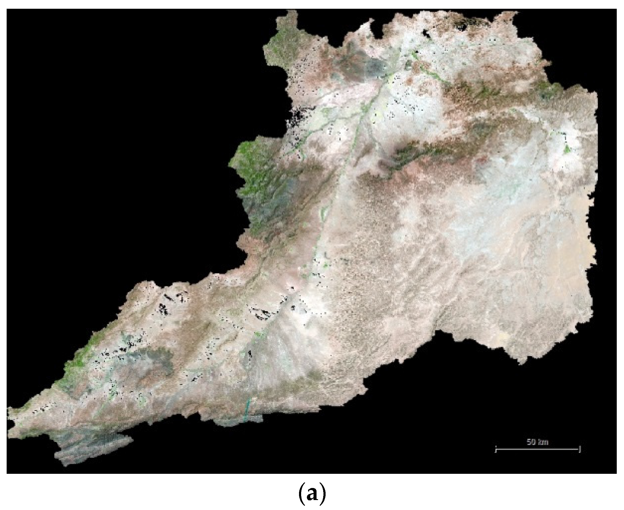
The study area encompassed the Moulouya River watershed upstream of the dam Mohammed V (Figure 1), the largest river basin in Morocco, covering about 55,000 km2. The Moulouya River is the chief river of Northeastern Morocco. Rising in the High Atlas mountains in central Morocco, it flows for around 600 km northeastward through a semiarid valley to the Mediterranean Sea just west of the Algerian border. Along its riverbed we can find the watershed that feeds the dam Mohammed V, consisting of a semiarid plain with low specific degradation in principle, though concentrated forms of erosion can be periodically reactivated.
The study site has a semiarid Mediterranean climate with relatively low and irregular annual rainfall (average annual values between 200 and 400 mm). Average temperatures usually range between 5 °C and 18 °C in the cold seasons and between 18 °C and 31 °C in hot weather.
According to FAO [31], the term “Forest” involves areas that span over more than 0.5 hectares of trees taller than 5 m and canopy cover of more than 10% (or areas of trees able to reach these characteristics in situ). This definition clearly excludes both agricultural and urban areas and shrubland and scrubland ecosystems. In the context of this work, and bearing in mind that we are dealing with Mediterranean arid and semiarid areas in which forest stands are sparse and frequently appear in the form of degraded bush that is clearly lower than 5 m in height, the term “Forest” has been slightly modified to account for forest stands larger than 0.5 hectares, containing trees taller than 2.5 m (as an estimated average height), and presenting a canopy cover of more than 10%. The so-called “alpha grass,” mainly composed of dense perennial herbs and dwarf shrubs such as Stipa tenacissima L. (esparto grass), covers most of the natural forests situated in Northeastern Morocco, representing a surface close to 2.2 million hectares. Another important LC (Land Cover) in the study area would be composed of shrubland vegetation such as Rosmarinus officinalis (rosemary), Lavandula dentate L. (fringed lavender), Thymus vulgaris (thyme), and aromatic and medicinal plants. The forested area, which is the target LC in this work, mostly consisting of conifers and some hardwood forests, represents only 9.4% of the total forest area in the region.
Figure 1. Location and delineation of the Moulouya River watershed upstream of the dam Mohammed V (UTM 30N projection and WGS84 reference system).
Forests 07 00023 g001

2.2. Data Sets

Satellite images were obtained from the NASA Landsat series [32], distributed by the USGS through the display GLOVIS (Global Visualization Viewer). To ensure complete coverage of the study area, five cloud-free Landsat L1T scenes were acquired for both 1984 (sensor Landsat 5 TM) and 2013 (sensor Landsat 8 OLI) (Table 1).
Table 1. Characteristics of the input data (Landsat images). Multispectral bands R, G, B, Nir, Swir1 and Swir2 (30 m ground pixel size) were used in all the cases.
SensorDateSensorDateFootprint: Path/Row
Landsat 5 TM27 August 1984Landsat 8 OLI26 July 2013200/36
Landsat 5 TM27 August 1984Landsat 8 OLI26 July 2013200/37
Landsat 5 TM27 August 1984Landsat 8 OLI26 July 2013200/38
Landsat 5 TM7 October 1984Landsat 8 OLI4 August 2013199/36
Landsat 5 TM7 October 1984Landsat 8 OLI4 August 2013199/37
The Level 1T (L1T) data product provides systematic radiometric and geometric corrections by incorporating ground control points (GCPs), while also employing a digital elevation model (DEM) to undertake terrain correction. L1T products had been previously orthorectified (UTM projection and WGS84 reference system) and corrected for terrain relief. Geodetic accuracy of these products depends on the accuracy of the ground control points and the resolution of the DEM used. According to the corresponding metadata files, the georeferencing mean error (expressed as RMSE2D or planimetric error computed at GCPs) was always notably lower than 30 m (i.e., subpixel error), which means that images may have been considered suitable for the purposes of the study.

3. Methods

3.1. Image Pre-Processing

Raw imagery (i.e., the original pixel digital values for every one of the spectral bands) has to be converted into valuable reflectance data, a critical element in vegetation mapping. Regarding the radiometric corrections, each image was converted from digital number to absolute spectral radiance (units of energy) and then to top of atmosphere spectral reflectance. Subsequently, top of atmosphere reflectance was converted to surface reflectance by applying atmospheric correction, which minimizes the effect of water vapor (humidity), aerosols (from dust, volcanoes, etc.), and other factors. In fact, since the atmospheric conditions at different acquisition dates influence spectral signatures, conversion from top of atmosphere reflectance to surface reflectance using a proper atmospheric calibration method should be accomplished, especially before conducting a change detection analysis [33].
In this case, a variation of the 6S atmospheric radiative transfer model [34], included in the software CLASlite [35], was applied. The 6S model simulates the atmosphere in each satellite image, modelling light passing through the atmosphere, interacting with the land surface, and returning through the atmosphere to the satellite sensor. It requires a number of inputs which include an estimate of aerosol optical thickness (AOT) and water vapor. Within CLASlite, these atmospheric parameters are held in geographic look-up tables derived from the NASA MODIS 1-degree atmospheric products.
Once radiometric and atmospheric corrections were performed on raw images, the five corrected ground reflectance images belonging to both 1984 and 2013 were mosaicked within the ArcGIS 10 environment to obtain the continuous dataset shown in Figure 2.
Figure 2. Orthorectified mosaics (UTM 30N WGS84) of ground reflectance values (RGB combination) covering the whole Moulouya River watershed upstream of the dam Mohammed V. (a) Landsat 5 TM images 1984; (b) Landsat 8 OLI images 2013.
Forests 07 00023 g002aForests 07 00023 g002b

3.2. Spectral Mixture Analysis (Subpixel Approach)

When medium and coarse spatial resolutions images are used for LC classification, mixed pixels are a major problem affecting mapping accuracy because of a lack of purity regarding spectral signatures. Spectral mixture analysis (SMA) is a common method for collecting subpixel information from fractional images [36]. In this case the key is to identify suitable endmembers for unmixing multispectral images into fractional ones [37]. In this work, SMA is performed to decompose image pixels into three principal components such as photosynthetic vegetation (PV; live vegetation at the level of the forest canopy), non-photosynthetic vegetation (NPV; dry carbon compounds such as dead vegetation, senescent vegetation, wood) and bare soil (S; exposed mineral soils, rocks, infrastructure). Regarding Landsat data, it has been proved that the majority of variation in a Landsat image (>98%) can be represented by a combination of three endmembers components [38]. In this sense, SMA has been successfully applied in semiarid ecosystems using Landsat TM data [39].
Most SMA approaches assume that image pixels contain endmember cover fractions that are linearly summed according to the following equation:
R ( λ ) = C P V R P V ( λ ) + C N P V R N P V ( λ ) + C S R S ( λ ) + ε
where R(λ) is the reflectance value of the observed pixel at wavelength λ and CPV, CNPV and CS are the percentages of fractional covers for the aforementioned principal constituents or endmembers, RPV(λ), RNPV(λ) and RS(λ) being the corresponding reflectance at wavelength λ for every one of the three endmembers considered. The term ε would encompass the error.
In this study, the applied SMA method relies on the Monte Carlo unmixing algorithm (AutoMCU). AutoMCU is a probabilistic approach based on the physical characteristics of the forest canopy developed by Asner et al. through different works [22,40,41,42,43]. AutoMCU unmixes the spectra of each pixel into 3 fractions of land cover (PV, NPV and S) using three spectral libraries gathered from field work and hyperspectral sensors that represent standard reflectance properties of PV, NPV and S components. The Monte Carlo approach randomly selects spectra from the PV, NPV, and S libraries and solves a set of linear equations, each of the form of the spectral unmixing Equation (1) but at a different wavelength. In this way, the process of random spectra selection from each library is repeated many times in each pixel until the unmixing equation is solved to obtain the final fractions corresponding to PV, NPV and S. In this work, the whole computation process was carried out by using CLASlite software [35].

3.3. Image Segmentation (Object-Based Approach)

Traditionally, change detection techniques have used individual pixels as their basic units of analysis, which we will refer to hereafter as pixel-based image analysis. While pixel-based image analysis is based on the information in each pixel, OBIA is based on information from a set of similar pixels called image objects. More specifically, image objects are groups of pixels in the image that represent meaningful objects in the scene because they are similar to one another based on a measure of spectral properties, such as size, shape, and texture, as well as context from a neighborhood surrounding the pixels [44]. In this sense, object-based methods can reduce the spectral variation within the same land covers.
In this work, object-based change detection is conducted by applying image segmentation and object-based classification to each one of the previously attained datasets (ground reflectance orthoimages corresponding to 1984 and 2013 shown in Figure 2).
The widely used multiresolution segmentation algorithm implemented in eCognition 8.8 [45] was utilized to create the objects from 1984 and 2013 Landsat orthomosaics. This is a general bottom-up segmentation algorithm based on region-merging and homogeneity definitions. It uses different homogeneity criteria based on several input parameters, such as scale, shape, compactness and band weights, all of which are related to the size and internal heterogeneity of the objects. The optimal determination of these three somewhat abstract parameters is not easy to carry out. A detailed explanation about the multiresolution segmentation algorithm has been previously published [45].
For the current work, the MS bands Red, Nir and Swir1 were used and equally weighted for each ground reflectance orthoimage from 1984 and 2013. The selection followed the recommendations proposed by Campbell et al. [24]. A systematic trial-and-error approach validated by the visual inspection of the quality of the output image objects has previously been carried out for setting the parameters required by the mutiresolution segmentation algorithm [46]. In this case, the shape and compactness parameters took values of 0.1 and 0.5 respectively, while the scale parameter was set at 50. After running the segmentation process, 593,144 and 616,021 image objects were segmented in the orthoimages of 2013 and 1984 respectively.

3.4. Features Vector Used to Carry Out Object-Based Classification

Several features were included in the classification process. The selected attributes were all computed at object level, i.e., an object-based features vector, comprising spectral information, vegetation indices and SMA derived features. The software eCognition v. 8.8 [47] was employed for the extraction of the object-based features from the Landsat orthoimages corresponding to 1984 and 2013. Therefore, a feature space formed by 22 object features categorized in three groups as defined in Table 2 was evaluated by the following criteria: (i) object spectral information based on mean and standard deviation values; (ii) four vegetation indices (VIs) widely applied in vegetation extraction and; (iii) mean and standard deviation values of SMA derived features such as PV, NPV and S fractions for every object. Other object features based on geometric properties such as shape index, density, etc. were not considered because they do not have a consistent contribution in the vegetation identification (e.g., [24]). Textural information has not been included in this study because its contribution to improve classification results is usually poor as compared to spectral features when working on medium resolution satellite images [48]. In fact, the combination of spectral and spatial classification is usually valuable for fine land-cover classification systems in areas with complex landscapes [49]. Moreover, the performance of a textural image varies with the complexity of the study area, the texture measure used, the size of moving window, and the image itself [50]; however, it is widely recognized that textural features are highly suitable for application in very high spatial resolution images [44]. It is worth mentioning that textural information was included in this study by means of standard deviation values, which can be considered as first-order textural features [51].
Table 2. Object attributes selected to characterize “Forest” and “Non-Forest” classes.
Type of FeatureNameDescription
Spectral (Landsat bands)Mean reflectance for Blue, Green, Red, Nir, Swir1, and Swir2 Landsat bandsMean value for every object computed from the corresponding reflectance values of all the pixels belonging to the same object [47]
Standard deviation reflectance for Blue, Green, Red, Nir, Swir1 and Swir2 Landsat bandsStandard deviation (SD) value for every object computed from the corresponding reflectance values of all the pixels belonging to the same object [47]
Vegetation indicesNDVI (Normalized Digital Vegetation Index) [52] N i r R e d N i r + R e d
MSR (Modified Simple Ratio) [53] Nir Red 1 ( Nir Red ) 0.5 + 1
NDSVI (Normalized Differential Senescent Vegetation Index) [54] Swir 1 Red Swir 1 + Red
GVI (Green Vegetation Index) [55] G r e e n R e d G r e e n + R e d
SMA derivedFraction PV, Fraction NPV and Fraction SoilMean value for every object computed from the corresponding SMA fraction of all the pixels belonging to the same object [47]
Standard deviation Fraction PV, Fraction NPV and Fraction SoilStandard deviation (SD) value for every object computed from the corresponding SMA fraction of all the pixels belonging to the same object [47]

3.5. Random Forest Classifier and Classification Accuracy Assessment

Random Forest (RF) was selected to undertake the classification of all the objects previously segmented (see Section 3.3). RF is an ensemble, supervised and non-parametric classifier in which a majority vote over several bootstrapped decision trees is carried out. The idea of a bootstrap is to sample the dataset (ground truth) with a replacement in order to form a training set. For this, a dataset of N instances is sampled N times. After building each decision tree, it is easy to demonstrate that, from a statistical point of view, around 2/3 of the available data will be used to train the classifier, leaving the remaining 1/3 as the test or validation dataset, which is also known as out-of-bag data (OOB). The accuracy of all OOB elements, or OOB accuracy, is an unbiased estimate of the overall classification accuracy and, therefore, an independent test data or cross-validation is not required when RF is employed [56].
RF has performed good classification accuracies in several remote sensing studies (e.g., [57,58]), proving to be relatively robust in spite of training size reduction and noise. Furthermore, the algorithm can estimate the importance of features for the general classification of the land-cover categories and for the classification of each category by means of the Gini Index and OOB estimation [57]. In this work, the Gini index, which measures the impurity of a given element with respect to the rest of the classes, has been used to maximize dissimilarity between classes in RF tree design by helping find the best split selection [59]. Gini measurements were computed as the sum of the products of all pairs of class proportions for classes present at the node. It reaches its maximum value when class sizes at the node are equal, and it is equal to zero if all cases in a node belong to the same class [59]. To assess the importance of each feature, the RF switches one of the input random variables while keeping the rest constant, and it measures the decrease in accuracy that has taken place by means of the OOB error estimation and of the Gini Index decrease [56].
The RF classifier only needs the definition of two parameters for generating a prediction model: the number of classification trees desired (K) and the number of prediction variables (P) used in each node to make the tree grow. Thus, to classify a new dataset, a constant number of P random predictive variables is used, and each of the examples of the dataset is classified by a K number of trees. This way, the final value of the class assigned to each example will be equal to the most frequent value for the total number of K trees generated. The value of P affects both the correlations between the trees and the strength of the individual trees. Reducing P reduces correlation and strength; increasing P increases both. Taking this into account, it is preferable to use a large number of trees (K) and a small number of split variables (P) to reduce the generalization error and the correlation between trees [57]. On the other hand, the number of trees necessary for good performance rises with the number of predictors. In this work, the required number of trees was experimentally tested by checking the OOB error as a function of the number of trees [57] and setting the number of random predictive variables in p = log2 (M + 1), M being the total number of predictor variables [60]. It was thereby found that OOB error remained stable above K = 100 trees. In other words, the addition of more trees neither increases nor decreases the generalization error. Thus, the parameter number of trees was set to 100 in this study.
STATISTICA v10 was used for the application of RF-based classification over a ground truth or reference dataset formed by 1310 objects extracted from the Landsat 2013 orthomosaic. Since the working area was covered by very high resolution and freely accessible Google Earth images collected in July 2013, it represented a very valuable resource for building up the required ground truth (Figure 3).
Due to the hypothesis of a much higher spectral variability in the case of the “Non-Forest” class, 832 “Non-Forest” and 478 “Forest” samples were randomly extracted from a larger database composed of both “Forest” and “Non-Forest” samples previously pre-classified by means of Google Earth (visual-based sampling). The selection of “Forest” and “Non-Forest” objects of the initial database was meant to cover as best as possible the spectral variability of both classes over the whole working area while maintaining a reasonable balance between them. Finally, the randomly extracted forest and non-forest samples were carefully checked by means of Google Earth and field work. Notice that there were some mixed samples (objects) containing forest and non-forest land cover. Those mixed samples were discarded if one fraction was not clearly majority with respect to each other. In those cases, and also when it was not clear whether the sample was consistent with our semantic definition of forest, field work was necessary to help improve the initial Google Earth based ground truth. This field work was carried out in September 2014 by visiting the location of questionable samples and checking the corresponding class by visual inspection.
Regarding the number of instances required to undertake a proper classification accuracy assessment, Congalton [61] suggested that 50 could be a proper number of samples per class when the scene is not too extensive, while a number from 75 to 100 would be advisable for vast areas or predominant classes. It is important to highlight that more than 100 samples for each target class have been allocated in the OOB dataset to carry out the accuracy assessment (Table 4 and Table 6).
Error matrices were calculated for each classification, and overall accuracy (OA), user’s accuracy (UA) and producer’s accuracy (PA) statistics were derived [61]. Additionally, in order to offer significance to the given results, intervals of confidence by the Exact method [62] were calculated (p < 0.05) because it corresponds to the maximum likelihood estimate (i.e., the actual value of the estimated accuracy OA, UA or PA), even when it is not symmetrical.
Figure 3. Image object classified as “Forest” overlaid on very high resolution Google Earth images corresponding to 2013.
Forests 07 00023 g003
Once the RF model trained and validated on the 2013 dataset was accepted, it was also applied to the 1984 image objects dataset to obtain the corresponding classification results. It is worth noting that most of the time it is completely impossible to count on a proper ground truth to train the classifier when working on old images (e.g., those taken in 1984). This is the reason why the need of normalizing the datasets has to be emphasized, that is correcting, both radiometrically and atmospherically, all the multitemporal datasets used. In this way, one of the ideas supporting this study lies in the fact that it is extraordinarily time-consuming and expensive, especially in developing countries, to carry out the ground reference required to train the classifier for every Landsat scene taken on different dates. Moreover, notice that the OBIA approach tends to mitigate pixel variability by computing features over homogeneous objects rather than isolated pixels.

4. Results and Discussion

4.1. Results from Random Forest Classification Including All Object-Based Features

A proper feature selection improves the performance of the classification process by identifying the most relevant features. It reduces the computational complexity and increases the generalization capability of the supervised classifier. The relative importance for the general classification of every feature extracted from the 2013 Landsat dataset according to RF classification and the Gini index is depicted in Table 3. It was found that many different types of features were regarded as important, although all object features based on standard deviation were poorly ranked. Moreover, PV, NPV and S fractions derived from SMA (subpixel approach), along with most vegetation indices, were ranked among the ten best features for “Forest” and “Non-Forest” classifications. Notice that NDVI is located at the top, demonstrating its ability to provide information about the density of green biomass, vegetation status and canopy structure in a given image object [63].
As previously reported by Asner and Heidebrecht [41], the Swir2 spectral region turns out to be one of the best ways to estimate the fractional cover of photosynthetic vegetation, non-photosynthetic vegetation and bare soils in arid regions. In fact, Mean Swir2 was ranked the third feature in relative importance, although it has also been somehow included in the computed fractions of PV, NPV and Soil obtained from SMA approach.
Table 3. Relative importance of every object-based feature according to Random Forest training stage (all object-based features were computed from 2013 Landsat dataset).
FeaturesRelative Importance
NDVI_2013100.00
Mean Green_201392.08
Mean Swir2_201390.53
MSR_201386.35
Fraction PV 201386.14
Mean Red_201382.57
Fraction Soil 201379.92
Mean Blue_201371.63
Fraction NPV 201371.57
GVI_201368.37
NDSVI_201368.34
Standard deviation Fraction NPV 201361.10
Standard deviation Fraction PV 201360.36
Mean Nir_201358.42
Mean Swir1_201355.06
Standard deviation Swir1_201345.58
Standard deviation Fraction Soil 201344.91
Standard deviation Nir_201341.44
Standard deviation Red_201337.58
Standard deviation Blue_201332.98
Standard deviation Swir2_201331.66
Standard deviation Green_201324.90
A summary of the results of the accuracy assessment, along with the 95% confidence intervals for each accuracy descriptor, is presented in Table 4. The overall accuracy (OA) took a value of 89.1%, statistically varying from 85.7% to 92.0%. Those results were considered to be suitable since the OA was always higher than 85%, which has been established as the minimum acceptable value for the classification results by different authors ([64,65]). That minimum seemed to be a reasonable reference for the required accuracy in this work since there was a large variability within the classes that were labelled.
The user’s accuracy (UA) for each target class indicated the expected error when using the classification map in field or commission error (Table 4). The reliability of the classification was very high for the class “Non-Forest”, with a probability of success greater than 91%. However, this probability was slightly lower in the case of the “Forest” class with a value of 84.7%.
The “Non-Forest” class also attained higher values than the “Forest” class with respect to the producer’s accuracy (PA) (Table 4), an accuracy measure related to error of omission that represents the probability of leaving without classifying a pixel belonging to one of the target classes. Briefly, and working with the whole object-based features vector, RF classifier performed worse when dealing with the “Forest” class, likely because of the unexpected high spectral variability of the vegetated ecosystems apparently included in this target class. Indeed, the complexity of landscapes and spectral confusion amongst the different land covers potentially constituting the “Forest” class (fruit crops, shrubland vegetation, croplands, Alpha grass and so on) helped to worsen the expected results.
Table 4. Classification accuracy assessment computed from the Random Forest out-of-bag subset (estimate of misclassification rate). The whole object-based features vector was used in training. Confidence Intervals (CI) were calculated at p < 0.05 signification level according to [62].
Classification Data Predicted by Random Forest ModelTotal
ForestNon-Forest
Observed Data (Ground Truth)Forest12222144
Non-Forest22238260
Total144260404
User’s accuracyProducer’s accuracyOverall accuracy
Forest84.7% (CI: 77.8% to 90.2%)84.7% (CI: 77.8% to 90.2%)89.1% (CI: 85.7% to 92.0%)
Non-Forest91.5% (CI: 87.5% to 94.6%)91.5% (CI: 87.5% to 94.6%)

4.2. Results from Random Forest Classification Only Including Object-Based Indices’ Features

As was said before, by extracting as much information as possible from a given data set while using the smallest number of features, we can save significant computation time and build models that generalize better for unseen data points. According to Yang and Honavar [66], the choice of features used to represent patterns that are presented to a classifier affects several pattern classification aspects, including the accuracy of the learned classification algorithm, the time needed for learning a classification function, the number of training instances needed for learning, and the cost associated with the features. In fact, if two numerical features are perfectly correlated, then one does not add any additional information to the machine learning process and only contributes with confusion, a phenomenon widely known as “the curse of dimensionality”. Thus, if the number of features is too high (relative to the training sample size), then it is usually beneficial to reduce the number of features through a feature space optimization technique based, for example, on the relative importance of every object-based feature, provided in Table 3. Furthermore, it seems reasonable to take advantage of those features computed as ratios (normalized values) more than those based on mean values of ground reflectance. This strategy could help to apply the obtained RF classification model to other Landsat datasets located at similar arid and semiarid areas regardless of the type of atmospheric correction carried out.
In this sense, the original feature space was significantly reduced from 22 features to only 7 based on four vegetation indices and three SMA derived fractions (PV, NPV and Soil). The relative importance of every feature belonging to this new features vector, again according to RF classification and the Gini index, is shown in Table 5. It is worth noting that NDVI continued being the most relevant feature, closely followed by the photosynthetic vegetation fraction provided by SMA approach. A little more detached is the feature fraction of soil.
Table 5. Relative importance of every object-based feature according to Random Forest training stage (only object-based indices’ features for 2013 Landsat dataset).
FeaturesImportance
NDVI_2013100.00
Fraction PV 201397.70
Fraction Soil 201383.43
GVI_201377.34
MSR_201375.31
NDSVI_201374.85
Fraction_NPV_201361.54
The results from applying RF classifier on the new reduced feature space can be observed in Table 6. It is relevant to underline a significant improvement of the initial classification accuracy results shown in Table 4, reaching an OA value of 92.3% with a minimum statistically estimated value of 89.3%. Similarly, the UA and PA indicator notably improved, both for the “Forest” and “Non-Forest” classes, denoting a better performance of the RF classifier working on a significantly reduced features vector. As has been previously reported, the RF classifier usually achieves high accuracy compared to other supervised classifiers such as maximum likelihood, spectral angle, single classification trees ([67,68]) and neural network [69], although there are other non-parametric classifiers that can overcome, in certain conditions, the results provided by RF, such as support vector machines [70]. Furthermore, the RF model provides quantitative measurements of each feature’s relative contribution to the classification result for users to evaluate the importance of input variables.
The accuracy results provided for the “Forest” class continued to be worse than those achieved in the case of the “Non-Forest” class, although they can be considered adequate to reasonably detect a change in the surface components of the vegetation cover or, additionally, spectral/spatial movement of vegetation in time, thereby generating location maps that help in the process of decision-making and possible intervention and correction works.
Table 6. Classification accuracy assessment computed from the Random Forest out-of-bag (estimate of misclassification rate). Only object-based indices’ features were used in training. Confidence intervals (CI) were calculated at p < 0.05 signification level according to [62].
Classification Data Predicted by Random Forest ModelTotal
ForestNon-Forest
Observed data (Ground Truth)Forest12715142
Non-Forest16247263
Total143262405
User’s accuracyProducer’s accuracyOverall accuracy
Forest88.8% (CI: 82.5% to 93.5%)89.4% (CI: 83.2% to 94.0%)92.3% (CI: 89.3% to 94.7%)
Non-Forest94.3% (CI: 90.7% to 96.8%)93.9% (CI: 90.3% to 96.5%)

4.3. Forest Cover Change between 1984 and 2013

The RF model calibrated from the 2013 Landsat dataset was directly applied to the 1984 Landsat dataset, allowing us to obtain binary maps “Forest-Non-Forest” for the Moulouya River watershed for the years 1984 and 2013 (Figure 4 and Figure 5 respectively).
From these maps, it could be estimated that the forest land cover in 1984 was close to 165,061 has, while in 2013 it was about 173,865 has. That meant a very small net increase of forest cover (5.3%) from 1984 to 2013, which can be qualified as a somewhat disappointing situation from the point of view of the aforementioned ten-year programme (2005–2014), meant to mitigate the risk and impact of deforestation processes in Morocco by undertaking an intense plan of reforestation.
Although difficult to pin down since the scheduled hectares for reforestation in the ten-year programme were related to provinces, and the Moulouya River watershed partly occupies several Moroccan ones, it was estimated that the reforested area planned in our working zone should be around 20,000–25,000 has, a value significantly higher than the data provided in this study. In brief, although the reforestation process is ongoing, it should be intensified over the years to come. It is beyond the scope of this article to review the consequences that the failure of this programme may have on the sustainability of the irrigated perimeters located downstream the Mohammed V dam, such as Triffa, Zebra, Garet and Bouareg areas, in the medium to long term.
Figure 4. Binary map Forest-Non-Forest for the Moulouya River watershed (area located upstream the dam Mohammed V) from Landsat image data corresponding to 1984.
Forests 07 00023 g004
Figure 5. Binary map Forest-Non-Forest for the Moulouya River watershed (area located upstream the dam Mohammed V) from Landsat image data corresponding to 2013.
Forests 07 00023 g005
The forested and non-forested areas presented in Figure 4 and Figure 5 can be compared to the results obtained by Hansen et al. [21], corresponding to Landsat image data taken in 2000 (Figure 6). It is interesting to note that the spatial distribution pattern of forested areas turned out to be quite similar, although data from Hansen et al. depicted a significantly smaller forest land cover comprising an area of about 62,995 has. It should be remembered that, according to our results, the forest land cover in 1984 was close to 165,061 has, while in 2013 it was about 173,865 has.
In fact, the study from Hansen et al., despite being very exhaustive and worldwide scale, necessarily tends to generalize with respect to canopy closure for all vegetation taller than 5 m. Notice that within the context of this study, and taking into account the singularity of forests located at arid and semiarid areas, the semantic definition of “Forest” has been slightly changed to only consider those containing trees taller than 2.5 m in average as forest stands. Therefore, global forest land cover maps should be carefully applied to regional or local scale, especially when dealing with arid and semiarid Mediterranean areas where forest stands are sparse and not very strong, and often appear in the form of degraded bush clearly shorter than 5 m. Hence, regarding studies of a more local type, it is important to count on appropriate training that enables the supervised classifier to discriminate between forested/reforested areas and “alpha grass”/shrubland ecosystems typical of semiarid regions.
Figure 6. Binary map Forest-Non-Forest for the Moulouya River watershed (30 m ground spatial resolution). Tree cover in the year 2000, defined as canopy closure for all vegetation taller than 5 m as average height. Data taken from Hansen et al. [21].
Forests 07 00023 g006

5. Conclusions

This study was intended as a methodological approach headed up to integrate subpixel-based (spectral mixture analysis; SMA) and pixel-based information (spectral values and vegetation indices) from Landsat data in the context of an object-based image analysis (OBIA) to efficiently map forest and non-forest areas located in arid and semiarid regions. Random Forest was applied to classify objects according to several object-based computed features.
The accuracy of the results attained in this work, especially the ability to work on a normalized and reduced set of features, makes our approach highly recommended to multi-temporal monitoring of forest evolution on a regional scale in arid and semiarid areas. Notice that most existing methods need the ground reference data to be collected for each image dataset, causing considerable cost in time and labor resources. If a trained classification algorithm could be utilized repeatedly for multiple years without the need for reformulation each year, mapping cost would be significantly reduced and the timeliness of the map products would be improved. Therefore, the approach proposed in this work, based on an innovative method using an OBIA, SMA and Random Forest classifier, has been successfully tested to automatically classify previously segmented multi-temporal Landsat imagery as forest or non-forest image objects. This information can be used to assess the efficacy of past actions and design future strategies to preserve and improve the vulnerable and scarce forests located in the working area.
It is beyond the scope of this paper to discuss the patterns or driving factors of the forest cover change in the Moulouya river watershed. This would require not only a quantitative net balance between forest and non-forest areas, but a spatially focused change detection study designed to locate spatial distribution of change detection results, or even a detailed “ from-to ” change trajectories study. This relevant issue should be addressed through rigorous and exhaustive further works.

Acknowledgments

This work has been supported and co-financed by the European Union under the European Regional Development Fund (FEDER) through the Cross-Border Cooperation Operational Programme Spain-External Borders 2008–2013 (Grant Reference 0065_COPTRUST_3_E). It also takes part of the general research lines promoted by the Agrifood Campus of International Excellence ceiA3 (further information can be retrieved from http://www.ceia3.es/). Thanks are also due to the Spanish Association of Graphic Engineering (INGEGRAF) for its financial contribution to the publication of this article. Finally, we also thank the three anonymous reviewers whose thorough and thoughtful reviews made the manuscript much stronger.

Author Contributions

Fernando J. Aguilar proposed the methodology, designed and conducted the experiments, and contributed extensively in manuscript writing and revision. Abderrahim Nemmaoui collected the input data, performed the experiments, and verified the results of the classification proposed in this study, additionally collaborating in manuscript writing and revision. Manuel A. Aguilar, Mimoun Chourak, Yassine Zarhloule and Andrés M. García Lorca made significant contributions to the research design and manuscript preparation, providing suggestions for the methodology design and conducting the data analysis and manuscript revision. Mimoun Chourak and Yassine Zarhloule also contributed with field work to help improve the initial Google-Earth-based ground truth.

Conflicts of Interest

The authors declare no conflict of interest.

References

  1. Dixon, R.K.; Houghton, R.A.; Solomon, A.M.; Trexler, M.C.; Wisniewski, J. Carbon pools and flux of global forest ecosystems. Science 1994, 263, 185–190. [Google Scholar] [CrossRef] [PubMed]
  2. Barker, T.; Bashmakov, I.; Bernstein, L.; Bogner, J.E.; Bosch, P.; Rutu, D.; Ogunlade, D.; Fisher, B.S.; Gupta, S.; Halsnaes, K.; et al. Technical Summary in Climate Change 2007: Mitigation. Contribution of Working Group III to the Fourth Assessment Report of the Intergovernmental Panel on Climate Change; Cambridge University Press: Cambridge, UK; New York, NY, USA, 2007. [Google Scholar]
  3. Nemmaoui, A.; García-Lorca, A.M.; Aguilar, F.J.; Aguilar, M.A. Time series of vegetation for a destroyed forest model. The case of Tadla Azilal (Morocco). Agrociencia 2013, 47, 267–280. [Google Scholar]
  4. Andréassian, V. Waters and forests: from historical controversy to scientific debate. J. Hydrol. 2004, 291, 1–27. [Google Scholar] [CrossRef]
  5. Geeson, N.A.; Brandt, C.J.; Thornes, J.B. Mediterranean Desertification: A Mosaic of Processes and Responses; John Wiley & Sons: England, UK, 2003. [Google Scholar]
  6. Saldaña, M.M.; Nemmaoui, A.; Cantón, M.Y.; Aguilar, M.A.; Aguilar, F.J. Estimation of the potential erosion in the Moulouya River watershed upstream of the dam Mohammed V. Mapping 2015, 168, 4–16. [Google Scholar]
  7. Rosenzweig, C.; Strzepek, K.M.; Major, D.C.; Iglesias, A.; Yates, D.N.; McCluskey, A.; Hillel, D. Water resources for agriculture in a changing climate: International case studies. Global Environ. Chang. 2004, 14, 345–360. [Google Scholar] [CrossRef]
  8. Orindi, V.A.; Murray, L.A. Adapting to Climate Change in East Africa: A Strategic Approach; Gatekeeper Series No. 117; International Institute for Environment and Development: London, UK, 2005. [Google Scholar]
  9. Dong, J.; Kaufmann, R.K.; Myneni, R.B.; Tucker, C.J.; Kauppi, P.E.; Liski, J.; Buermann, W.; Alexeyev, V.; Hughes, M.K. Remote sensing estimates of boreal and temperate forest woody biomass: Carbon pools, sources, and sinks. Remote Sens. Environ. 2003, 84, 393–410. [Google Scholar] [CrossRef]
  10. Hudiburg, T.; Law, B.; Turner, D.P.; Campbell, J.; Donato, D.; Duane, M. Carbon dynamics of Oregon and Northern California forests and potential land-based carbon storage. Ecol. Appl. 2009, 19, 163–180. [Google Scholar] [CrossRef] [PubMed]
  11. Luyssaert, S.; Schulze, E.D.; Borner, A.; Knohl, A.; Hessenmoller, D.; Law, B.E.; Ciais, P.; Grace, J. Old-growth forests as global carbon sinks. Nature 2008, 455, 213–215. [Google Scholar] [CrossRef] [PubMed]
  12. Balderas Torres, A.; Ontiveros Enríquez, R.; Skutsch, M.; Lovett, J.C. Potential for Climate Change Mitigation in Degraded Forests: A Study from La Primavera, Mexico. Forests 2013, 4, 1032–1054. [Google Scholar] [CrossRef]
  13. Stephens, P.; Watt, P.; Loubser, D.; Haywood, A.; Kimberley, M. Estimation of carbon stocks in New Zealand planted forests using airborne scanning lidar. International Archives of Photogrammetry. Remote Sens. Spat. Inf. Sci. 2007, 36, 389–394. [Google Scholar]
  14. Boulmane, M.; Makhloufi, M.; Bouillet, J.P.; Saint-André, L.; Satrani, B.; Halim, M. Estimation du stock de carbone organique dans les Quercus ilex du Moyen Atlas Marocain. Acta Bot. Gallica 2010, 157, 451–467. [Google Scholar] [CrossRef]
  15. Hansen, M.C.; Loveland, T.R. A review of large area monitoring of land cover change using Landsat data. Remote Sens. Environ. 2012, 122, 66–74. [Google Scholar] [CrossRef]
  16. Xian, G.; Homer, C.; Fry, J. Updating the 2001 National Land Cover Database land cover classification to 2006 by using Landsat imagery change detection methods. Remote Sens. Environ. 2009, 113, 1133–1147. [Google Scholar] [CrossRef]
  17. Wulder, M.A.; Franklin, S.E. Understanding Forest Disturbance and Spatial Pattern: Remote Sensing and GIS Approaches; Taylor & Francis: Boca Ratón, FL, USA, 2007. [Google Scholar]
  18. Kennedy, R.E.; Yang, Z.; Cohen, W.B. Detecting trends in forest disturbance and recovery using yearly Landsat time series: 1. LandTrendr-Temporal segmentation algorithms. Remote Sens. Environ. 2010, 114, 2897–2910. [Google Scholar] [CrossRef]
  19. Huang, C.; Goward, S.N.; Schleeweis, K.; Thomas, N.; Masek, J.G.; Zhu, Z. Dynamics of national forests assessed using the Landsat record: Case studies in eastern United States. Remote Sens. Environ. 2009, 113, 1430–1442. [Google Scholar] [CrossRef]
  20. Pang, C.; Yu, H.; He, J.; Xu, J. Deforestation and Changes in Landscape Patterns from 1979 to 2006 in Suan County, DPR Korea. Forests 2013, 4, 968–983. [Google Scholar] [CrossRef]
  21. Hansen, M.C.; Potapov, P.V.; Moore, R.; Hancher, M.; Turubanova, S.A.; Tyukavina, A.; Thau, D.; Stehman, S.V.; Goetz, S.J.; Loveland, T.R.; et al. High-Resolution Global Maps of 21st-Century Forest Cover Change. Science 2013, 342, 850–853. Available online: http://earthenginepartners.appspot.com/science-2013-global-forest (accessed on 15 December 2015). [Google Scholar] [CrossRef] [PubMed]
  22. Robertson, L.D.; King, D.J. Comparison of pixel- and object-based classification in land cover change mapping. Int. J. Remote Sens. 2011, 32, 1505–1529. [Google Scholar] [CrossRef]
  23. Vieira, M.A.; Formaggio, A.R.; Rennó, C.D.; Atzberger, C.; Aguiar, D.A.; Mello, M.P. Object Based Image Analysis and Data Mining applied to a remotely sensed Landsat time-series to map sugarcane over large areas. Remote Sens. Environ. 2012, 123, 553–562. [Google Scholar] [CrossRef]
  24. Campbell, M.; Congalton, R.G.; Harter, J.; Ducey, M. Optimal Land Cover Mapping and Change Analysis in Northeastern Oregon Using Landsat Imagery. Photogramm. Eng. Remote Sens. 2015, 81, 37–47. [Google Scholar] [CrossRef]
  25. Fisher, P. The pixel: A snare and a delusion. Int. J. Remote Sens. 1997, 18, 679–685. [Google Scholar] [CrossRef]
  26. Cracknell, A.P. Synergy in remote sensing—What’s in a pixel? Int. J. Remote Sens. 1998, 19, 2025–2047. [Google Scholar] [CrossRef]
  27. Foody, G.M.; Cox, D.P. Sub-pixel land cover composition estimation using a linear mixture model and fuzzy membership functions. Int. J. Remote Sens. 1994, 15, 619–631. [Google Scholar] [CrossRef]
  28. Woodcock, C.E.; Gopal, S. Fuzzy set theory and thematic maps: Accuracy assessment and area estimation. Int. J. Geogr. Inf. Sci. 2000, 14, 153–172. [Google Scholar] [CrossRef]
  29. Asner, G.P.; Lobell, D.B. A biogeophisical approach for automated SWIR unmixing of soils and vegetation. Remote Sens. Environ. 2000, 74, 99–112. [Google Scholar] [CrossRef]
  30. Haut Commissaire aux Eaux et Forêts et à la Lutte Contre la Désertification. Bilan des Réalisations du Programme Décennal (2005–2009); HCEFLCD/DPSIC/DSI/SSE: Rabat, Morocco, 2009. Available online: http://www.eauxetforets.gov.ma/admin/telechargement/fr/Bilan_2005_2009_programme_d%C3%A9cennal_forestier.pdf (accessed on 9 July 2014).
  31. FAO. Global Forest Resources Assessment Update 2005. Terms and Definition. Forest Resources Assessment Programme; Working Paper 83; FAO: Roma, Italy, 2005. [Google Scholar]
  32. Woodcock, C.E.; Allen, R.; Anderson, M.; Belward, A.; Bindschadler, R.; Cohen, W.B.; Gao, F.; Goward, S.N.; Helder, D.; Helmer, E.; et al. Free access to Landsat imagery. Science 2008, 320, 1011. [Google Scholar] [CrossRef] [PubMed]
  33. Song, C.; Woodcock, C.E.; Seto, K.C.; Lenney, M.P.; Macomber, S.A. Classification and change detection using Landsat TM data: When and how to correct atmospheric effects? Remote Sens. Environ. 2001, 75, 230–244. [Google Scholar] [CrossRef]
  34. Vermote, E.F.; Tanre, D.; Deuze, J.L.; Herman, M.; Morcrette, J.J. Second simulation of the satellite signal in the solar spectrum, 6S: An overview. IEEE Trans. Geosci. Remote Sens. 1997, 35, 675–686. [Google Scholar] [CrossRef]
  35. Asner, G.P.; Knapp, D.E.; Balaji, A.; Páez-Acosta, G. Automated mapping of tropical deforestation and forest degradation: CLASlite. J. Appl. Remote Sens. 2009, 3, 1–24. [Google Scholar] [CrossRef]
  36. Lu, D.; Moran, E.; Hetrick, S. Detection of impervious surface change with multi-temporal Landsat images in an urban-rural frontier. ISPRS J. Photogramm. Remote Sens. 2011, 66, 298–306. [Google Scholar] [CrossRef] [PubMed]
  37. Lu, D.; Moran, E.; Batistella, M. Linear mixture model applied to Amazonian vegetation classification. Remote Sens. Environ. 2003, 87, 456–469. [Google Scholar] [CrossRef] [Green Version]
  38. Small, C. The Landsat ETM+ spectral mixing space. Remote Sens. Environ. 2004, 93, 1–17. [Google Scholar] [CrossRef]
  39. Elmore, A.J.; Mustard, J.F.; Manning, S.J.; Lobell, D.B. Quantifying vegetation change in semiarid environments. Remote Sens. Environ. 2000, 44, 87–102. [Google Scholar] [CrossRef]
  40. Asner, G.P. Biophysical and biochemical sources of variability in canopy reflectance. Remote Sens. Environ. 1998, 64, 234–253. [Google Scholar] [CrossRef]
  41. Asner, G.P.; Heidebrecht, K.B. Spectral unmixing of vegetation, soil and dry carbon cover in arid regions: comparing multispectral and hyperspectral observations. Int. J. Remote Sens. 2002, 23, 3939–3958. [Google Scholar] [CrossRef]
  42. Asner, G.P.; Keller, M.; Pereira, R.; Zweede, J.C.; Silva, J.N. Canopy damage and recovery after selective logging in Amazonia: Field and satellite studies. Ecol. Appl. 2004, 14, 280–298. [Google Scholar] [CrossRef]
  43. Asner, G.P.; Knapp, D.E.; Broadbent, E.N.; Oliveira, P.J.C.; Keller, M.; Silva, J.N. Selective logging in the Brazilian Amazon. Science 2005, 310, 480–482. [Google Scholar] [CrossRef] [PubMed]
  44. Blaschke, T. Object based image analysis for remote sensing. ISPRS J. Photogramm. Remote Sens. 2010, 65, 2–16. [Google Scholar] [CrossRef]
  45. Baatz, M.; Schäpe, A. Multiresolution segmentation. In Angewandte Geographische Informationsverarbeitung XII: Beiträge zum AGIT-Symposium Salzburg 2000 (German Edition); Strobl, J., Blaschke, T., Griesebner, G., Eds.; Wichmann-Verlag: Heidelberg, Germany, 2000; pp. 12–23. [Google Scholar]
  46. Tian, J.; Chen, D.M. Optimization in multi-scale segmentation of high-resolution satellite images for artificial feature recognition. Int. J. Remote Sens. 2007, 28, 4625–4644. [Google Scholar] [CrossRef]
  47. Trimble Germany GmbH. eCognition Developer 8.8 Reference Book; Trimble Germany GmbH: Munich, Germany, 2012. [Google Scholar]
  48. Peña-Barragán, J.M.; Gutiérrez, P.A.; Hervás-Martínez, C.; Six, J.; Plant, R.E.; López-Granados, F. Object-based image classification of summer crops with machine learning methods. Remote Sens. 2014, 6, 5019–5041. [Google Scholar] [CrossRef]
  49. Lu, D.; Weng, Q. A survey of image classification methods and techniques for improving classification performance. Int. J. Remote Sens. 2007, 28, 823–870. [Google Scholar] [CrossRef]
  50. Chen, D.; Stow, D.A.; Gong, P. Examining the effect of spatial resolution and texture window size on classification accuracy: An urban environment case. Int. J. Remote Sens. 2004, 25, 2177–2192. [Google Scholar] [CrossRef]
  51. Aguilar, M.A.; Vallario, A.; Aguilar, F.J.; García Lorca, A.; Parente, C. Object-Based greenhouse horticultural crop identification from multi-temporal satellite imagery: A case study in Almeria, Spain. Remote Sens. 2015, 7, 7378–7401. [Google Scholar] [CrossRef]
  52. Rouse, J.W.; Haas, R.H.; Schell, J.A.; Deering, D.W. Monitoring vegetation systems in the Great Plains with ERTS. In Proceedings of the Earth Resources Technology Satellite Symposium NASA SP-351, Washington, DC, USA, 10–14 December 1973; Volume 1, pp. 309–317.
  53. Chen, J. Evaluation of vegetation indices and modified simple ratio for boreal applications. Can. J. Remote Sens. 1996, 22, 229–242. [Google Scholar] [CrossRef]
  54. Qi, J.; Marsett, R.; Heilman, P.; Biedenbender, S.; Moran, S.; Goodrich, D. RANGES improves satellite-based information and land cover assessment in southwest United States. Trans. Am. Geophys. Union 2002, 83, 601–606. [Google Scholar] [CrossRef]
  55. Gitelson, A.A.; Kaufman, Y.J.; Stark, R.; Rundquist, D. Novel algorithms for remote estimation of vegetation fraction. Remote Sens. Environ. 2002, 80, 76–87. [Google Scholar] [CrossRef]
  56. Breiman, L. Random forest. Mach. Learn. 2001, 45, 5–32. [Google Scholar] [CrossRef]
  57. Rodríguez-Galiano, V.F.; Ghimire, B.; Rogan, J.; Chica-Olmo, M.; Rigol-Sánchez, J.P. An assessment of the effectiveness of a random forest classifier for land-cover classification. ISPRS J. Photogramm. Remote Sens. 2012, 67, 93–104. [Google Scholar] [CrossRef]
  58. Smith, A. Image segmentation scale parameter optimization and land cover classification using the Random Forest algorithm. J. Spat. Sci. 2010, 55, 69–79. [Google Scholar] [CrossRef]
  59. Breiman, L.; Friedman, J.; Stone, C.J.; Olshen, R.A. Classification and Regression Trees, 1st ed.; Chapman and Hall/CRC: Belmont, CA, USA, 1984. [Google Scholar]
  60. Hill, T.; Lewicki, P. Statistics: Methods and Applications; StatSoft: Tulsa, OK, USA, 2007. [Google Scholar]
  61. Congalton, R.G. A review of assessing the accuracy of classifications of remotely sensed data. Remote Sens. Environ. 1991, 37, 35–46. [Google Scholar] [CrossRef]
  62. Sauro, J.; Lewis, J.R. Estimating completion rates from small samples using binomial confidence intervals: Comparisons and recommendations. In Proceedings of the Human Factors and Ergonomics Society 49th annual meeting, Orlando, FL, USA, 26–30 September 2005; pp. 2100–2104.
  63. Turner, D.P.; Cohen, W.B.; Kennedy, R.E.; Fassnacht, K.S.; Briggs, J.M. Relationships between Leaf Area Index and Landsat TM Spectral Vegetation Indices across three temperate zone sites. Remote Sens. Environ. 1999, 70, 52–68. [Google Scholar] [CrossRef]
  64. Congalton, R.G.; Green, K. Assessing the Accuracy of Remotely Sensed Data, 2nd ed.; CRC Press: Boca Ratón, FL, USA, 2009. [Google Scholar]
  65. Foody, G.M. Status of land cover classification accuracy assessment. Remote Sens. Environ. 2002, 80, 185–201. [Google Scholar] [CrossRef]
  66. Yang, J.; Honavar, V. Feature subset selection using a genetic algorithm. IEEE Intell. Syst. 1998, 13, 44–49. [Google Scholar] [CrossRef]
  67. Lawrence, R.L.; Wood, S.D.; Sheley, R.L. Mapping invasive plants using hyperspectral imagery and Breiman Cutler classifications (Random Forest). Remote Sens. Environ. 2006, 100, 356–362. [Google Scholar] [CrossRef]
  68. Na, X.; Zhang, S.; Li, X.; Yu, H.; Liu, C. Improved land cover mapping using random forest combined with Landsat Thematic Mapper imagery and ancillary geographic data. Photogramm. Eng. Remote Sens. 2010, 76, 833–840. [Google Scholar] [CrossRef]
  69. Chan, J.C.; Paelinckx, D. Evaluation of random forest and AdaBoost tree-based ensemble classification and spectral band selection for ecotope mapping using airborne hyperspectral imagery. Remote Sens. Environ. 2008, 112, 2999–3011. [Google Scholar] [CrossRef]
  70. Mountrakis, G.; Im, J.; Ogole, C. Support vector machines in remote sensing: A review. ISPRS J. Photogramm. Remote Sens. 2011, 66, 247–259. [Google Scholar] [CrossRef]

