Using Spatial Optimization to Create Dynamic Harvest Blocks from LiDAR-Based Small Interpretation Units

Abstract

Spatial and temporal differences in forest features occur on different scales as forest ecosystems evolve. Due to the increased capacity of remote sensing methods to detect these differences, forest planning may now consider forest compartments as transient units which may change in time and depend on the management objectives. This study presents a methodology for implementing these transient units, referred to as dynamic treatment units (DTU). LiDAR (Light Detecting and Ranging) data and field sample plots were used to estimate forest stand characteristics for 500-m² pixels and compartments, and a set of models was developed to enable growth simulations. The DTUs were obtained by maximizing a utility function which aimed at maximizing the aggregation of harvest areas and the ending growing stock volume with even-flow cutting targets for three 10-year periods. Remote sensing techniques, modeling, simulation, and spatial optimization were combined with the aim of having an efficient methodology for assigning cutting treatments to forest stands and delineating compact harvest blocks. Pixel-based planning led to more accurate estimation of stand characteristics and more homogeneity inside the delineated harvest blocks while the compartment-based planning resulted in larger and higher area/perimeter ratio.

1. Introduction

Forest management planning should aim towards efficiently achieving the management objectives set for a given forest area [1]. Detailed and accurate knowledge on the existing forest resources in the target area is needed for developing optimal forest management plans [2]. In this regard, the increasing use of LiDAR (Light Detection and Ranging) has led to new approaches in forest inventory since the 1960s [3] when this technology was first applied to the estimation of forest variables [4]. This is leading to new approaches also in forest management planning with the aim of increasing the efficiency of the management of forest resources.

LiDAR sensors provide a cloud of georeferenced data points from which spatial and structural information can be obtained in order to characterize the vegetation and the terrain of an area of interest. Using an area-based approach [5], one can obtain spatially continuous forest inventory data. High-resolution technologies such as LiDAR make it possible to greatly improve the spatial resolution and accuracy of forest inventories [6]. LiDAR has been shown to provide reliable estimates of stand characteristics such as forest cover [7], biomass and carbon stock [8], crown base height, and stand basal area and volume [9], and tree diameter distribution [10]. The resulting calculation units (e.g., pixels [11] or micro-stands [12]) may be spatially organized using computational methods. For example, cuttings may be aggregated or dispersed [13], and ecological corridors may be created [14].

The traditional forest management approach assumes fixed and predefined boundaries for forest compartments or other treatment units. The approach based on dynamic treatment units (DTU) allows the treatment units to evolve in time based on the spatial variation in the stand. The use of LiDAR gives the possibility to increase the resolution of both forest inventory and management planning as compared to the traditional approach [15], even with low pulse density data [16]. Dynamic treatment units can be derived from LiDAR-based information using spatial optimization methods [16,17,18]. Heuristic methods have been increasingly used in spatial forest planning problems [19] and they have reached satisfactory solutions at a reasonable computational cost [20,21]. Among the existing heuristic optimization techniques, simulated annealing (SA) has proven suitable to deal with the aggregation of small calculation units into larger cutting areas [22].

The aim of this study was to implement a forest management planning methodology based on the utilization of dynamic treatment units in Mediterranean pine forests using LiDAR to estimate forest information at present state. At the first step, a set of models were developed for simulating the stand dynamics. Then, the performance of two approaches was assessed: when calculation units were either predefined compartments or pixels. In both cases, harvests were aggregated using spatial optimization. The study provides insights into state-of-the-art forest planning methods that may be generalized to any forest ecosystem worldwide in order to improve the efficiency of forestry by using transient treatment units.

2. Materials and Methods

2.1. Study Area

The study area is Forest #76, a public forest located within the Model Forest of Urbión in San Leonardo de Yagüe (Soria province, central Spain), which is also a part of the Mediterranean Model Forest Network (Figure 1). The area has a long tradition of intensive forest management based on traditional forest planning methods. The Urbión forest area is the most extensive forest of the Iberian Peninsula, covering more than 100,000 hectares. Pinus sylvestris L. and Pinus pinaster Ait. are the main tree species in the area. Forest #76 covers 221.7 ha hectares (UTM30N coordinates: 479786–478042 West-East; 4635486–4633630 South-North). The average altitude is 1179 m above sea level (1122 m–1243 m) while slope ranges from 0° to 45° (mean slope 7.56°). Southern aspect is more frequent (25.4% of the area) than northern exposures (8.4%). High physiographic variability results in differences in soil characteristic and site quality throughout the study area.

2.2. Forest Inventory

LiDAR data were used in combination with field sample plots to develop local models for predicting stand variables (i.e., number of trees per hectare, stand basal area, and stand volume) for the inventory units. The field work was carried out during autumn 2010 when 44 circular plots of 12.6 m radius (500 m²) were established with the aim of covering all forest types existing in the area. The coordinates of the center of each plot were measured using a global navigation satellite system device (Trimble R6) for precise positioning. Calipers and a hypsometer (Vertex III) were used to measure all trees in every plot for their diameter at breast height (DBH), total height, and height of tree crown. In addition, the ages of 44 trees, a dominant tree in each plot, were measured. On average, each plot contained 33 trees. The proportion of each pine species in each plot was used to divide Forest #76 into two strata: the “Pinaster” stratum (i.e., pure Pinus pinaster stands) and the “Mixed” stratum (i.e., mixed Pinus sylvestris and Pinus pinaster stands) (

Table 1. Summary of field plot data.

Measured variables	Pinaster stratum			Mixed stratum
	30 Sample Plots
	Min	Mean	Max	Min	Mean	Max
Diameter at breast height (cm)	7.1	14.8	22.0	6.3	12.8	19.3
Tree height (m)	7.1	14.8	22.0	6.3	12.8	19.3
Stand density (trees·ha−1)	260.0	604.0	1080.0	360.0	797.1	1440.0
Stand basal area (m2·ha−1)	21.2	47.4	72.1	12.9	31.6	59.2
Stand volume (m3·ha−1)	102.1	363.9	640.0	76.9	219.2	463.3
Dominant height (m)	11.9	17.3	21.8	10.7	15.2	19.0
Age (year)	33.0	56.4	74.0	33.0	42.4	78.0

).

LiDAR data were collected using ALS60 II sensor in 10 April 2014 with a pulse density of 2 points per square meter. Software FUSION [23] was used to compute a large array of LiDAR-derived metrics as detailed in [24]. The stand variables measured from the field sample plots were used as dependent variables in non-linear regression analysis, while selected LiDAR metrics were used as independent variables. The selection of predictors was based on previous literature on similar cases and correlation tests between y-response variables and candidate predictors. The models were fitted to the data using R software [25]. To estimate the stand variables of the case study, models were used with LiDAR metrics calculated for a 22.4-m square grid (500 m²), since this cell size is equal to the plot size (12.6 m radius). This resolution was considered acceptable for this study as the number of trees in each plot was large enough (slightly higher than 30), but different resolutions can be analyzed in further studies.

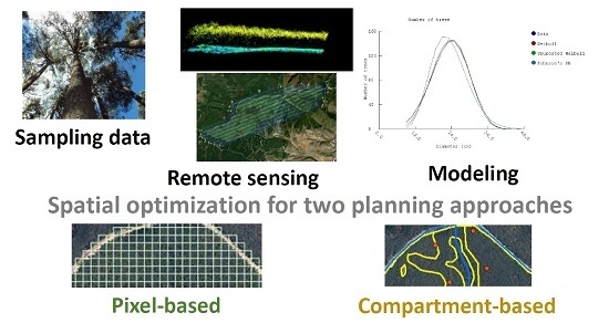
2.3. Stand Delineation

The available spatial information representing the traditional forest management approach consisted of 13 stands, the mean area of which was 17.1 ha (10.3–25.8 ha), and 17 vegetation units (i.e., forest types) differing in stand age, species composition, and/or stand structure. The mean size of the vegetation units was 12.6 ha, ranging from 0.5 to 49.4 ha. Forest compartments (i.e., calculation units in the so-called traditional forest planning) were obtained as the overlay of the two layers, resulting in 68 compartments (Figure 2).

The pixel-based inventory and planning approach used a continuous grid of 500-m² pixels. Stand basal area and number of trees per hectare were predicted for each pixel using models developed in this study. In the compartment approach, the characteristics of each compartment were calculated as the mean of those LiDAR pixels. To avoid the edge effect, we did not consider pixels that were only partly within a compartment.

2.4. Diameter Distribution Modelling

Since the simulation of treatment alternatives was based on individual-tree models, knowledge on the diameter distribution within each calculation unit was required. Therefore, a diameter distribution model was developed based on the truncated two-parameter Weibull density function [26]:

$$f\left(d\right)=\frac{c}{b}{\left(\frac{d}{b}\right)}^{c-1}\exp \left({\left(\frac{t}{b}\right)}^c-{\left(\frac{d}{b}\right)}^c\right)\left(t\le d\le \infty , t,c,b>0\right),$$

(1)

where t is the truncation point (7.5 cm), b is the scale parameter, c is the shape parameter, and d is DBH. The function is truncated at 7.5 cm because this is the lowest measured diameter in the plots.

The parameters of the Weibull density function were estimated by fitting the distribution function to the diameter distribution data of each plot using maximum likelihood. Then, models for the scale and shape parameters were fitted through linear regression analysis. The fitting data consisted of 54 pairs of b and c values. The number of diameter distributions fitted was larger than the number of inventory plots because in mixed stands the diameter distributions were fitted separately for Pinus pinaster and Pinus sylvestris.

2.5. Growth Modelling

Models for predicting the stand dynamics of both species on an individual-tree basis were developed using data from the 2nd and 3rd National Forest Inventory (NFI) of Soria and Burgos provinces. The model set consisted of the following models: (i) diameter-increment; (ii) survival; (iii) height-diameter relationship; and (iv) ingrowth. Tree growth and survival were modeled as a function of competition, tree size, and site quality. The modelling database comprised 11,883 living and 602 dead trees of Pinus pinaster, and 18,411 living and 657 dead trees of Pinus sylvestris. The ingrowth model consisted of two sub-models, one predicting the number of trees per hectare that pass the 7.5-cm limit and the other predicting the mean diameter of ingrowth trees at the end of the 10-year period. The number of ingrowth trees was 764 for Pinus pinaster and 912 for Pinus sylvestris.

Since stand age was available only for very few NFI plots (age was recorded only for plantations) it was not possible to develop age-dominant height models or use stand age or site index as a predictor in the growth models. Therefore, a growth index [27] was computed instead of site index based on the ratio between the measured and the predicted past growth of trees in the NFI plots. The growth index describes the fertility of the site (i.e., its growth potential). However, unlike the NFI plots, past growth measurements were not available for the inventory plots of the case study area. Instead, stand age and dominant height were available. Therefore, the past growth index based on diameter increment was replaced by a growth index based on the ratio between the measured and predicted dominant height. A local model for dominant height development was fitted for this purpose using the inventory plots of the study area and the guide curve method [28]. Three models (i.e., Hossfeld I, modified Hossfeld I, and Chapman-Richards) were tested using the 44 age and dominant height values. The dominant height at the pixel level was estimated using the regression models based on LiDAR metrics, while the dominant height for a compartment was calculated as the mean of all pixel estimates within the compartment perimeter.

2.6. Forest Planning and Spatial Optimization

The planning horizon was set to 30 years and divided into three 10-year periods. In combinatorial optimization it is necessary to define a range of reasonable treatment alternatives for each calculation unit. This was achieved by using three different rotation lengths, three thinning basal areas, and three thinning intensities, leading to 27 combinations (27 simulation rules). The thinning basal area (i.e., the maximum stand basal area allowed prior to thinning) and the corresponding diameter at which final felling should be done were calculated based on the three site index classes observed in our forest. Rotation diameter increased as site index decreased, as trees need more time to reach the same status compared to more productive areas. We used a 2% discount rate to determine whether the stand was financially mature (i.e., ready to cut) or not. Moreover, each rule was used with eight different settings concerning whether cutting is allowed during a certain 10-year period (from 000 = no cuttings to 111 = cutting allowed during every period). Therefore, 8 times 27 simulations representing even-aged management were done for each calculation unit (i.e., either pixels or predefined compartments), and all simulations that produced a different management schedule were maintained. In addition, 8 times 9 schedules representing uneven-aged management were simulated for each stand. The nine different simulation rules were obtained by combining three different thinning basal area levels with three different thinning intensities. In uneven-aged management cuttings were simulated as high thinning, using larger harvest rates for larger diameter classes.

Spatial optimization in forest management planning can be conducted through the maximization or minimization of a utility function getting values from 0 to 1 (Equations (2) and (3)). In the case of multiple management objectives, the total utility can be expressed as the weighted sum of the sub-utility functions of the management goals [21,29]. The forest planning problem can be described as follows:

$$\text{max }U={\sum }_{i=1}^I{a}_i u_i \left(q_i\right)$$

(2)

subject to

q_i = Qi (X), i = 1,…, I

(3)

where U is total utility, a_i is the weight of sub-utility function u_i, and q_i is the quantity of objective variable i. Q_i is the procedure which calculates the value of objective variable i from the information of those treatment schedules that are included in the solution, and X is a vector that contains the code numbers of those schedules that are included in the solution. Sub-utility functions scale all objective variables to the range 0–1.

The following forest management objectives, defined by means of sub-utility functions, were considered in this study: (i) maximizing growing stock volume at the end of the third 10-year period (V₃₀); (ii) cutting exactly 10,000 m³ during each 10-year period (H₁, H₂, H₃); (iii) maximization of cut–cut borders of adjacent forest units (CC); and (iv) minimization of cut–non-cut borders of adjacent calculation units (CNC). Further details on sub-utility functions and their shapes in typical forest planning problems can be found [30]. Cut-cut border is the boundary between two adjacent spatial units which are both cut during the same 10-year period, and cut–non-cut border is the boundary between adjacent units of which one is cut and the other is not cut during a certain 10-year period. Objectives iii and iv both aggregate cuttings but, while the maximization of CC border creates large and continuous harvest blocks, minimization of CNC border leads to compact and circular shapes of the treatment units.

Preliminary tests were used to assign optimal weights to each of the objectives. Once periodical cuttings targets were met, the maximum possible weight was given to CNC to both maximize the isolation among harvest blocks and minimize the presence of isolated pixels, which is not practical in real forestry. The final weights used for the management objectives were: (i) V₃₀ 0.05; (ii) periodic cuttings 0.05 each, 0.15 overall; (iii) CC 0.05; and (iv) CNC 0.75. The following additive utility function was used:

U = 0.05 u₁ (V₃₀) + 0.05 u₂ (H₁) + 0.05 u₃ (H₂)+ 0.05 u₄ (H₃)+ 0.05 u₅ (CC)+ 0.75 u₆ (CNC),

(4)

The optimization algorithm used was simulated annealing (SA) which checks candidate solutions within the specified neighborhood [31]. This technique has been successfully applied in previous studies to solve spatial planning problems [30,32]. SA begins with an initial solution which is the best of a certain number of random combinations of treatment schedules of calculation units. The algorithm checks whether a candidate move would improve the utility function value. In the algorithm used in this study, a move consisted of simultaneous changes in the management schedules of two randomly selected pixels or compartments. The move was accepted if it improved the utility function value, otherwise the previous solution was kept. Inferior solutions (moves that decrease the utility value) were accepted with a small probability (described in [30]), and this probability was decreased during the optimization run. Because SA has stochastic elements, the results of different optimization runs may vary slightly. Thus, several trials are required to check the influence of the intrinsic randomness of the optimization procedure on the results. Based on existing literature [22], five repeated optimizations were carried out to reach the global optimum for each planning problem.

Once the spatial optimizations were ready, the treatment units that consisted of squared-shaped pixels were smoothed in order to produce more realistic DTU boundaries. The smoothing was carried out using the Polynomial Approximation with Exponential Kernel (PAEK) algorithm implemented in ArcGIS 10.2.1 [33]. In the PAEK algorithm, the smoothing depends on a tolerance factor. We used 100 m as the tolerance factor. A shape index (defined as the ratio between perimeter and area of cutting areas) was calculated for each harvest block as an indicator of the compactness of harvest blocks. After that, the efficiency of DTUs based on either predefined compartments or pixels was reassessed by introducing a minimum size criterion for the harvest blocks. We assumed 0.5 ha (i.e., 10 pixels) as the minimum allowed cutting area. The standard deviation of stand basal area for the pixels within each harvest block was used as a measure of the homogeneity of the harvest blocks.

3. Results

3.1. LiDAR-Based Models for Predicting Stand Attributes

The stand-level attributes were predicted using the following models:

H_o = 2.96 Elev_P90^0.8464 Int_P95^0.1089,

(5)

G = FC ^0.4183 Elev_P20^0.7545 Int_P05^0.1089,

(6)

V = FC ^0.3002 Elev_Mean^−1.6721 Int_P05^−0.1070,

(7)

N = 181.76 + FC^2.5417 Elev_P95^−1.6616 Int_P10^−0.1933,

(8)

where H₀ is the dominant height (m), G is the stand basal area (m²·ha⁻¹), V is the growing stock volume (m³·ha⁻¹), and N is the stand density (trees·ha⁻¹). The following predictors were used: FC: forest cover (percentage of first returns above 2-m height-break); Elev_P20, Elev_P90, Elev_P95: 20th, 90th and 95th percentile value of the height distribution of LiDAR pulses, respectively; Elev_Mean: mean height value for canopy return pulses; Int_P05, Int_P10 and Int_P95: 5th, 10th and 95th percentile value of canopy intensity returns, respectively.

The degree of explained variance was high for dominant height (R² = 0.906, RMSE = 1.17), growing stock volume (R² = 0.971, RMSE = 52.46), and stand basal area (R² = 0.809, RMSE = 6.89), and somewhat lower for stand density (R² = 0.640, RMSE = 206.98).

3.2. Diameter Distribution Models

The models for predicting parameters b and c of the truncated Weibull distribution were as follows:

• Pinus pinaster

  b = 98.119 − 15.593 lnN + 14.822 lnG − 0.018 ln(0.01 A),

  (9)

  c = 2.902 − 1.264 Dq + 1.377 b,

  (10)
• Pinus sylvestris

  b = 16.253 − 12.018 lnN + 12.249 lnG + 0.039 ln(0.01 A)

  (11)

  c = 4.49 − 0.514 Dq + 0.533 b,

  (12)

where N is the stand density, G is the stand basal area (m²·ha⁻¹), A is the altitude above sea level of the plot in meters, and Dq is the quadratic mean diameter (cm). The goodness of fit of the model for parameter b was considerably high (R² = 0.97, RMSE = 1.008 for Pinus pinaster, and R² = 0.94, RMSE = 1.645 for Pinus sylvestris) and was reasonably good for parameter c (R² = 0.45, RMSE = 1.607 for Pinus pinaster, and R² = 0.64, RMSE = 0.856 for Pinus sylvestris).

3.3. Growth Models

The Hossfeld I model (Equation (13)) was selected as the guide curve (average dominant height development) using stand age, in years, as the independent variable

$$H_0=\frac{Ag{e}^2}{-3.895+1.345 Age+0.039 Ag{e}^2}$$

(13)

The fitted Hossfeld I model proved to be statistically and biologically consistent for the study site conditions. The predicted dominant height accurately reflected the average development of the sample plots for the age interval of interest (20–80 years). The ratio between the inventory unit’s dominant height and its guide curve value was used as the growth index when Equations (14)–(19) were used to simulate stand development.

The models for the future 10-year over-bark diameter increment in centimeters (I_d) and 10-year survival probability (s) were as follows:

• Pinus pinaster

  $$I_d=1.128 ex{p}^{(1.537 - 0.022 d- 0.095 \frac{BAL}{ln\left(d +1\right)}+ 0.033 BA{L}_{thinned}+ 0.485 GI) }$$

  (14)

  $$s=\frac{1}{1+exp\left(-\left(-1.940-0.0144\frac{BAL}{ln\left(d+1\right)}+0.069 BA{L}_{thinned}+2.548 ln\left(0.01 A\right)\right)\right)}$$

  (15)
• Pinus sylvestris

  $$I_d=1.117 ex{p}^{(0.894 - 0.023 d - 0.088 \frac{BAL}{ln\left(d +1\right)} + 0.033 BA{L}_{thinned}+ 0.561 GI + 0.00026 A) }$$

  (16)

  $$s = \frac{1}{1+\exp \left(-\left(3.293+0.038 d-0.122 \frac{BAL}{ln\left(d+1\right)}+0.033 BA{L}_{thinned}\right)\right)}$$

  (17)

where d is the DBH (cm), BAL is the basal area of trees larger than the subject tree (m²·ha⁻¹), BAL_thinned is the basal area of larger trees thinned during the past 10-year period (m²·ha⁻¹), GI is the growth index of the plot, and A is the altitude in meters. The Snowdon Correction factor [34] was used to remove the backtransformation bias due to the use if log scale.

The diameter increment models predicted decreasing increments with increasing diameter for both species. For a given diameter, higher diameter increments were predicted for Pinus pinaster than for Pinus sylvestris. The predicted diameter growth increased with increasing site quality, as defined by the GI. In addition, competition appeared as a significant factor for diameter growth, decreasing diameter increment. The models explained only 27.6% to 33.4% of the variation in diameter increment, which can be partly explained by measurement errors (diameter increment was obtained as the difference of two independent measurements, both of which have inaccuracies).

According to the survival model results, higher survival rates can be expected for Pinus pinaster than for Pinus sylvestris. Thicker trees have higher probability of survival, whereas increasing competition experienced by a tree results in lower survival rates. Both species showed similar behaviour towards competition (BAL). Predicting the mortality at the individual-tree level is unreliable (R² was less than 0.1 in both cases) but, from the forest planning point of view, mortality at the stand level is more important. Thinning had a positive effect on the survival of the remaining trees.

The height-diameter models were as follows:

• Pinus pinaster

  $$h=\frac{61.058-0.165 GI-44.474 ln\left(A\right)+0.06207 A}{{\left(1+\frac{1912.431}{d^2}\right)}^{0.468}}$$

  (18)
• Pinus sylvestris

  $$h=\frac{-28.889-0.627 GI+35.445ln\left(A\right)–0.02889 A}{{\left(1+\frac{765.697}{d^2}\right)}^{0.623}}$$

  (19)

where h is tree height (m), GI is the growth index, A is the altitude above sea level in meters and d is the DBH (cm). The height-diameter model predicts higher height for Pinus sylvestris than for Pinus pinaster. DBH values ranging from 10 cm to 25 cm correspond to height values 6.1 m to 19.1 m for Pinus pinaster, and from 6.2 to 20.2 m for Pinus sylvestris if GI is set to 1 and altitude is 1200 m. The models explained 63% (Pinus sylvestris) and 70% (Pinus pinaster) of the variance in tree height.

It was also necessary to model the ingrowth for the lower diameter classes and the diameter of the ingrowth trees. The developed models for predicting the number of ingrowth trees at the end of the 10-year period (Fin, trees·ha⁻¹) and their mean diameter (Din, cm) were as follows:

• Pinus pinaster

  $$F_{in}= -295.5+112.3 ln\left(N\right)-139.3 ln\left(G\right)+1524.6 \frac{Gspe}{G}$$

  (20)

  $$D_{in}= -2.186+1.569 ln\left(N\right)-0.152 G$$

  (21)
• Pinus sylvestris

  $$F_{in}= -320.2+119.3 ln\left(N\right)-152.7 ln\left(G\right)+1681.5 \frac{Gspe}{G}$$

  (22)

  $$D_{in}= -0.45+1.150 ln\left(N\right)-0.152 G$$

  (23)

where N is stand density (trees·ha⁻¹), G is the stand basal area (m²·ha⁻¹), and Gspe is the basal area of the species for which ingrowth is predicted (m²·ha⁻¹). The number of ingrowth trees and their mean diameter decreased with increasing stand basal area for both species. The number of stems per hectare and the Gspe/G ratio (i.e., the proportion of basal area of the species) had a positive effect on the number of ingrowth trees. The goodness of fit was rather low for both models and both species (R² values less than 0.25 in the four cases) due to the randomness of ingrowth and the small size of the sample plots.

3.4. DTU Results: Pixels versus Predefined Compartments

The results for the forest planning formulation indicated that the periodical cutting targets for the three 10-year periods were fulfilled in both cases. The CC and CNC sub-utility function values cannot be compared directly because the total boundary length is very different for the compartment-based and the pixel-based planning. The computation of growing stock volume at the end of the 30-year period resulted in similar total values (only 3.1% higher when the optimization was based on compartments instead of pixels). However, the distribution of the total volume among treatment types showed significant differences that affect the spatial layout of resulting harvest blocks. The harvest blocks corresponding to the highest utility function value registered during the five repetitions for each planning problem (0.9189 for pixels and 0.8923 for compartments) are displayed in Figure 3 in order to visually compare the cutting areas defined for each period and planning problem.

Cutting treatments, consisting of three thinning intensities and two final cutting treatments for mature forests, totalled up to 256.6 ha in the compartment-based optimization, while 313.3 ha were cut in the pixel-based optimization (

Table 2. Treated area (hectares) by type along the forest management plan using either pixels or compartments as calculation units.

Treatment	2014–2023		2024–2033		2034–2043		Total
	Pixel	Comp	Pixel	Comp	Pixel	Comp	Pixel	Comp
Light thinning	32.8	40.0	52.3	17.2	56.6	18.4	141.7	75.6
Moderate thinning	16.9	36.4	16.7	12.2	19.5	0.0	53.1	48.6
Heavy thinning	0.7	0.0	1.8	11.7	0.3	10.5	2.8	22.2
Seed tree cut	30.1	23.1	39.0	32.9	9.3	21.5	78.4	77.5
Remove overstory	0.0	0.0	4.9	0.0	32.2	32.9	37.1	32.9
Total	80.5	99.5	114.7	74.0	117.9	83.3	313.3	256.8

). Differences in the light thinning treatment mainly accounted for the cutting areas between the two problems, being 141.7 ha in the pixel-based approach and 75.6 ha in the compartment-based approach.

In the optimization results displayed in Figure 3, 33 aggregations were created for pixels (without considering any minimum harvest block size) and 5 for compartments. The mean harvest block size using compartments (49.97 ha) was higher than using pixels (9.47 ha). The shape index was lower for compartment-based aggregation (0.007) than pixel-based aggregation (0.011). This means that compartment-based DTUs required shorter perimeters to cover the same treatment area than when pixels were used as calculation units. Since assuming very small harvest blocks may not be realistic, the results were also computed after introducing a minimum harvest block size of 0.5 ha. Now the number of harvest blocks based on the pixel-based approach was 17 (mean area of 18.3 ha), which resulted in a shape index of 0.0087. The standard deviation of stand basal area within harvest blocks composed of pixels was lower than within the harvest blocks of compartment-based planning (Figure 3). For example, the area-weighted average of the standard deviations of stand basal area was 11.7 m²·ha⁻¹ for pixel-based harvest blocks and 15.0 m²·ha⁻¹ for compartment-based harvest blocks.

4. Discussion

The models developed for stand attributes showed good accuracy in the prediction of growing stock volume and basal area, as found in other studies [4]. The use of ALS-based forest inventories has solid scientific support and it can lead to more accurate estimates of forest characteristics than the classic forest inventory methods [5]. Large-scale inventories based on low-density LiDAR data, such as our data, usually rely on an area-based approach and gridding [35] to estimate stand-level attributes. Further improvements may be achieved either by using an enhanced area-based approach [36] or by applying individual-tree detection methods [3] for denser point cloud data.

Our models reflected a slightly more bell-shaped diameter distribution in the monospecific Pinus pinaster stands as compared with mixed stands of Pinus pinaster and Pinus sylvestris. The parameters of the distribution function were similar to those obtained in previous research for the same species in a different region [37]. Also, the developed growth models showed similar height-diameter relationships as previous models [38], but the level of accuracy of our height-diameter models was slightly lower than in earlier studies [39,40].

The two forest management planning approaches evaluated in this study resulted in similar growing stock volume at the end of the planning horizon, but the prescriptions necessary to fulfill the cutting targets, as well as the number of harvest blocks, differed considerably between the two planning alternatives compared in this study. Previous research suggests that efficiency of forestry can be improved if boundary delineation is based on interpreted LiDAR data [41] and segmentation methods [42] rather than relying on traditional compartment-based approaches based on predefined stands. In the current study, the result was not so clear as in [22] The described traditional procedure resulted in non-homogeneous compartments, which were assumed homogeneous in the calculations. This most probably led to overestimated growth predictions because if a compartment is composed of sparse and dense patches, their average growth is less than the growth of an average patch of a homogeneous compartment (this is because of the non-linear relationship between stand density and growth). The use of compartments results in losses in the information gained by LiDAR-based inventory, as management units are not defined according to stand-level information but are based on predefined boundaries. Therefore, it may be assumed that the pixel-based DTU approach was more precise in terms of growth predictions and more accurate than the compartment-based alternative.

Small-sized gridding improves the spatial accuracy in locating thinning areas [43]. In addition, the results showed that the pixel-based approach resulted in efficient clustering of cuttings. However, some of the harvest blocks may be too small for practical implementation due to the highly fragmented forest in the southern limit of the study area, which consists of forest patches surrounded by non-forested area (Figure 2). The presence of gaps inside a forest area can cause bias and make it more difficult to achieve good aggregation of calculation units to delineate harvest blocks [16]. In general, the proportion of isolated small harvest blocks was low and these blocks were located in a specific fragmented area. The aggregations presented were more homogenous in terms of stand basal area for the approach based on pixels as compared to the compartment-based DTU (Figure 3).

Decentralized methods could be used in further research to reduce the computational cost of the centralized heuristics in large spatial planning problems. These methods can cope with both global (i.e., forest level) and local (i.e., calculation unit level) planning objectives. Cellular automata [44] and the spatial version of the reduced cost method [45], which both represent decentralized computing methods, have been used to aggregate harvest areas [46], with better harvest block shapes than obtained with centralized heuristics. However, isolated pixels may also appear when decentralized methods are used [16]. Among the centralized heuristic methods, genetic algorithms and tabu search have also been used to aggregate harvested raster cells units resulting in good levels of clustering [20,30]. Another alternative to heuristic techniques is to use exact solution techniques, such as mixed integer programming [47]: this technique was applied to a 22,100-ha forest using the k-nearest neighbor method to estimate stand characteristics. The clustering results indicated satisfactory levels of grouping. However, the dispersion of small-size harvest areas in fragmented forest areas was the shortcoming of the method.

More compactness in harvest areas leads to more efficient harvesting operations with less perimeter [48]. In the absence of constraints concerning the minimum size of treatment units, the compartment-based approach was more efficient in the aggregation of management units. However, the harvest blocks of the compartment-based approach cannot always be treated uniformly in all places, which means, for instance, that their shape indices give a too favorable picture of compartment-based planning. A solution to this problem might be the use of larger but homogeneous calculation units, such as segments or microsegments [16], which are more homogeneous than traditional compartments and more practical than pixels in the estimation of stand-level attributes.

5. Conclusions

This research presented a set of growth models for mixed pine forests in Central Spain to be applied in a forest planning system based on dynamic treatment units. The presented method for creating DTUs from small calculation units can be easily integrated with LiDAR-based forest inventory data to enhance the management of forest ecosystems. The comparison between forest planning approaches (pixels vs. compartments) showed that the homogeneity of the delineated harvest blocks was better in the pixel-based planning. However, the size and area/perimeter ratio of the harvest blocks were better for the compartment approach.

References

1. Kangas, A.; Kangas, J.; Kurttila, M. Introduction. In Decision Support for Forest Management; Managing Forest Ecosystems; Springer: Berlin, Germany, 2008; Volume 16, pp. 1–18. [Google Scholar]
2. Pukkala, T. Introduction to multi-objective forest planning. In Managing Forest Ecosystems: Multi-Objective Forest Planning; Managing Forest Ecosystems; Kluwer Academic Publishers: Dordrecht, The Netherlands, 2002; Volume 6, pp. 1–21. [Google Scholar]
3. Vauhkonen, J.; Maltamo, M.; McRoberts, R.E.; Næsset, E. Introduction to forestry applications of airborne laser scanning. In Forestry Applications of Airborne Laser Scanning: Concepts and Case Studies; Managing Forest Ecosystems; Springer: Berlin, Germany, 2014; Volume 27, pp. 1–21. [Google Scholar]
4. Rempel, K.C.; Parker, A.K. An information note on an airborne laser terrain profiler for micro-relief studies. In Proceedings of the 3rd Symposium on Remote Sensing of Environment; University of Michigan Institute of Science and Technology: Michigan, MI, USA, 1964; pp. 321–337. [Google Scholar]
5. Hyyppä, J.; Hyyppä, H.; Leckie, D.; Gougeon, F.; Yu, X.; Maltamo, M. Review of methods of small-footprint airborne laser scanning for extracting forest inventory data in boreal forests. Int. J. Remote Sens. 2008, 29, 1339–1366. [Google Scholar] [CrossRef]
6. Næsset, E. Area-based inventory in Norway. In Forestry Applications of Airborne Laser Scanning: Concepts and Case Studies; Managing Forest Ecosystems; Springer: Berlin, Germany, 2014; Volume 27, pp. 215–240. [Google Scholar]
7. Næsset, E.; Gobakken, T.; Holmgren, J.; Hyyppä, H.; Hyyppä, J.; Maltamo, M. Laser scanning of forest resources: the Nordic experience. Scand. J. For. Res. 2004, 19, 482–499. [Google Scholar] [CrossRef]
8. Smith, A.M.S.; Falkowski, M.J.; Hudak, A.T.; Evans, J.S.; Robinson, A.P.; Steele, C.M. A cross-comparison of field, spectral, and LiDAR estimates of forest canopy cover. Can. J. Remote Sens. 2009, 35, 447–459. [Google Scholar] [CrossRef]
9. García, M.; Riaño, D.; Chuvieco, E.; Danson, F.M. Estimating biomass carbon stocks for a Mediterranean forest in central Spain using LiDAR height and intensity data. Remote Sens. Environ. 2010, 114, 816–830. [Google Scholar] [CrossRef]
10. González-Olabarria, J.; Rodríguez, F.; Fernández-Landa, A.; Mola-Yudego, B. Mapping fire risk in the Model Forest of Urbión (Spain) based on airborne LiDAR measurements. For. Ecol. Manag. 2012, 282, 145–156. [Google Scholar] [CrossRef]
11. Maltamo, M.; Gobakken, T. Predicting tree diameter distributions. In Forestry Applications of Airborne Laser Scanning: Concepts and Case Studies; Managing Forest Ecosystems; Springer: Berlin, Germany, 2014; Volume 27, pp. 177–192. [Google Scholar]
12. Lu, F.; Eriksson, L. Formation of harvest units with genetic algorithms. For. Ecol. Manag. 2000, 130, 57–67. [Google Scholar] [CrossRef]
13. Pippuri, I.; Kallio, E.; Maltamo, M.; Peltola, H.; Packalén, P. Exploring horizontal area-based metrics to discriminate the spatial pattern of trees and need for the first thinning using airborne laser scanning. Forestry 2012, 85, 305–314. [Google Scholar] [CrossRef]
14. Bettinger, P.; Johnson, D.L.; Johnson, K.N. Spatial forest plan development with ecological and economic goals. Ecol. Model. 2003, 169, 215–236. [Google Scholar] [CrossRef]
15. Strunk, J.; Temesgen, H.; Andersen, H.E.; Flewelling, J.P.; Madsen, L. Effects of lidar pulse density and sample size on a model-assisted approach to estimate forest inventory variables. Can. J. Remote Sens. 2014, 38, 644–654. [Google Scholar] [CrossRef]
16. Magnusson, M.; Fransson, J.E.S.; Holmgren, J. Effects on estimation accuracy of forest variables using different pulse density of laser data. For. Sci. 2007, 53, 619–626. [Google Scholar]
17. Packalén, P.; Heinonen, T.; Pukkala, T.; Vauhkonen, J.; Maltamo, M. Dynamic treatment units in Eucalyptus plantation. For. Sci. 2011, 57, 416–426. [Google Scholar]
18. De-Miguel, S.; Pukkala, T.; Pasalodos, J. Dynamic treatment units: flexible and adaptive forest management and planning by combining spatial optimization methods and LiDAR. Cuadernos de la Sociedad Española de Ciencias Forestales 2013, 37, 49–54. [Google Scholar]
19. Pukkala, T.; Páckalen, P.; Heinonen, T. Dynamic treatment units in forest management planning. In The Management of Industrial Forest Plantations: Theoretical Foundations and Applications; Springer: Berlin, Germany, 2014; Volume 33, pp. 372–392. [Google Scholar]
20. Baskent, E.Z.; Keles, S. Spatial forest planning: A review. Ecol. Model. 2005, 188, 145–173. [Google Scholar] [CrossRef]
21. Lu, F.; Eriksson, L. Formation of harvest units with genetic algorithms. For. Ecol. Manag. 2000, 130, 57–67. [Google Scholar] [CrossRef]
22. Pukkala, T.; Kurttila, M. Examining the performance of six heuristic optimisation techniques in different forest planning problems. Silva Fenn. 2005, 39, 567–80. [Google Scholar] [CrossRef]
23. Pukkala, T.; Heinonen, T. Optimizing heuristic search in forest planning. Nonlinear Anal. 2006, 7, 1284–1297. [Google Scholar] [CrossRef]
24. McGaughey, R.J.; Carson, W.W. FUSION LIDAR data, photographs, and other data using 2D and 3D visualization techniques. In Proceedings of the Terrain Data: Applications and Visualization—Making the Connection, Charleston, SC, USA, 28 October 2003; American Society for Photogrammetry and Remote Sensing: Bethesda, MD, USA, 2003; pp. 16–24. [Google Scholar]
25. Valbuena, R.; Maltamo, M.; Packalen, P. Classification of multilayered forest development classes from low-density national airborne lidar datasets. Forestry 2016, 89, 392–401. [Google Scholar] [CrossRef]
26. R Core Team. R: A language and environment for statistical computing. R Foundation for Statistical Computing: Vienna, Austria, 2013; Available online: http://www.R-project.org/ (accessed on 20 March 2014).
27. Bailey, R.L.; Dell, T.R. Quantifying diameter distributions with the Weibull function. For. Sci. 1973, 19, 97–104. [Google Scholar]
28. Trasobares, A.; Pukkala, T. Using past growth to improve individual-tree diameter growth models for uneven-aged mixtures of Pinus. sylvestris L. and Pinus. nigra Arn. in Catalonia, north-east Spain. Ann. For. Sci. 2004, 61, 409–417. [Google Scholar] [CrossRef]
29. Clutter, J.L.; Fortson, J.C.; Pienaar, L.V.; Brister, G.H.; Bailey, R.L. Timber Management: A Quantitative Approach; John Wiley & Sons: Hoboken, NJ, USA, 1983. [Google Scholar]
30. Heinonen, T. Developing Spatial Optimization in Forest Planning. Master's Thesis, University of Joensuu, Joensuu, Finland, 2007. [Google Scholar]
31. Heinonen, T.; Pukkala, T. A comparison of one- and two-compartment neighborhoods in heuristic search with spatial forest management goals. Silva Fenn. 2004, 38, 319–332. [Google Scholar]
32. Dowsland, K.A. Simulated annealing. In Modern Heuristic Techniques for Combinatorial Problems; John Wiley & Sons: Hoboken, NJ, USA, 1993; pp. 20–63. [Google Scholar]
33. Öhman, K.; Eriksson, L.O. Allowing for spatial consideration in long-term forest planning by linking linear programming with simulated annealing. For. Ecol. Manag. 2002, 161, 221–230. [Google Scholar] [CrossRef]
34. ESRI (Environmental Systems Resource Institute). ArcMap 10.2.1. Smooth Line Command within Data Management Tool; ESRI: Redlands, CA, USA, 2014. [Google Scholar]
35. Snowdon, P. A ratio estimator for bias correction in logarithmic regressions. Can. J. For. 1991, 21, 720–724. [Google Scholar] [CrossRef]
36. Næsset, E. Determination of mean tree height of forest stands using airborne laser scanner data. J. Photogramm. Remote Sens. 1997, 52, 49–56. [Google Scholar] [CrossRef]
37. Packalén, P.; Strunk, J.L.; Pitkänen, J.A.; Temesgen, H.; Maltamo, M. Edge-Tree correction for predicting forest inventory attributes using area-based approach with airborne laser scanning. J. STARS 2015, 8, 1274–1280. [Google Scholar] [CrossRef]
38. Palahí, M.; Pukkala, T.; Trasobares, A. Modelling the diameter distribution of Pinus sylvestris, Pinus nigra and Pinus halepensis forest stands in Catalonia using the truncated Weibull function. Forestry 2006, 79, 553–562. [Google Scholar] [CrossRef]
39. Bravo-Oviedo, A.; Río, M.; Montero, G. Site index curves and growth model for Mediterranean maritime pine (Pinus pinaster Ait.) in Spain. For. Ecol. Manag. 2004, 201, 187–197. [Google Scholar] [CrossRef]
40. Palahí, M.; Miina, J.; Montero, G.; Pukkala, T. Individual-tree growth and mortality models for Scots pine (Pinus sylvestris L.) in north-east Spain. Ann. For. Sci. 2003, 60, 1–10. [Google Scholar] [CrossRef]
41. Lizarralde, I. Dinámica de Rodales y Competencia en las Masas de Pino Silvestre (Pinus sylvestris L.) y Pino Negral (Pinus pinaster Ait.) de los Sistemas Central e Ibérico Meridional. Ph.D. Thesis, University of Valladolid, Victoria, Spain, 2008. [Google Scholar]
42. Pascual, C.; García-Abril, A.; García-Montero, L.G.; Martín-Fernández, S.; Cohen, W.B. Object-based semi-automatic approach for forest structure characterization using lidar data in heterogeneous Pinus sylvestris stands. For. Ecol. Manag. 2008, 255, 3677–3685. [Google Scholar] [CrossRef]
43. Pekkarinen, A. A method for the segmentation of very high spatial resolution images of forested landscapes. Int. J. Remote Sens. 2002, 23, 2817–2836. [Google Scholar] [CrossRef]
44. Næsset, E.; Bjerknes, K.O. Estimating tree heights and number of stems in young forest stands using airborne laser scanner data. Remote Sens. Environ. 2001, 78, 328–340. [Google Scholar] [CrossRef]
45. Heinonen, T.; Pukkala, T. The use of cellular automaton approach in forest planning. Can. J. For. Res. 2007, 37, 2188–2200. [Google Scholar] [CrossRef]
46. Pukkala, T.; Heinonen, T.; Kurttila, M. An application of a reduced cost approach to spatial forest planning. For. Sci. 2009, 55, 13–22. [Google Scholar]
47. Mathey, A.H.; Nelson, J. Decentralized forest planning models—A cellular automata framework. In Designing Green Landscapes; Springer: Berlin, Germany, 2008; Volume 15, pp. 69–185. [Google Scholar]
48. Öhman, K.; Eriksson, L.O. Aggregating harvest activities in long term forest planning by minimizing harvest area perimeters. Silva Fenn. 2010, 44, 77–89. [Google Scholar] [CrossRef]
Figure 1. Study area: (a) Location of Soria and Burgos provinces; (b) Study area location
Forests 07 00220 g001
Figure 2. Stand delineation: (a) Distribution of sample plots and stand delineation made by local managers considering forest type cartography; (b) Forest inventory grid for the Pinaster stratum with the compartments resulting from the combination of compartment and forest type layers
Forests 07 00220 g002
Figure 3. Cutting areas for the first (a); second (c); and third (e) period using pixels as calculation units as well as cutting areas for the first (b); second (d); and third (f) period using compartments. Standard deviation of the stand basal area at the harvest block level is shown beside the largest harvest blocks.
Forests 07 00220 g003aForests 07 00220 g003b