Article

Estimation of Voxel-Based Above-Ground Biomass Using Airborne LiDAR Data in an Intact Tropical Rain Forest, Brunei

1
Department of Climate Environment, Korea University, Seoul 02841, Korea
2
Department of Environmental Science and Ecological Engineering, Korea University, Seoul 02841, Korea
3
Eco, Environment, Education (E3) Co., Ltd., Seoul 07547, Korea
4
Environmental and Life Sciences , Faculty of Science, Universiti Brunei Darussalam, Bandar Seri Begawan BE1410, Brunei Darussalam
*
Author to whom correspondence should be addressed.
Forests 2016, 7(11), 259; https://doi.org/10.3390/f7110259
Submission received: 27 July 2016 / Revised: 23 October 2016 / Accepted: 25 October 2016 / Published: 31 October 2016

Abstract

:
The advancement of LiDAR technology has enabled more detailed evaluations of forest structures. The so-called “Volumetric pixel (voxel)” has emerged as a new comprehensive approach. The purpose of this study was to estimate plot-level above-ground biomass (AGB) in different plot sizes of 20 m × 20 m and 30 m × 30 m, and to develop a regression model for AGB prediction. Both point cloud-based (PCB) and voxel-based (VB) metrics were used to maximize the efficiency of low-density LiDAR data within a dense forest. Multiple regression model AGB prediction performance was found to be greatest in the 30 m × 30 m plots, with R2, adjusted R2, and standard deviation values of 0.92, 0.87, and 35.13 Mg∙ha−1, respectively. Five out of the eight selected independent variables were derived from VB metrics and the other three were derived from PCB metrics. Validation of accuracy yielded RMSE and NRMSE values of 27.8 Mg∙ha−1 and 9.2%, respectively, which is a reasonable estimate for this structurally complex intact forest that has shown high NRMSE values in previous studies. This voxel-based approach enables a greater understanding of complex forest structure and is expected to contribute to the advancement of forest carbon quantification techniques.

1. Introduction

In recent years, awareness of forests under climate change has reached unprecedented levels [1]. The United Nations Framework Convention on Climate Change (UNFCCC) has introduced the REDD+ program, which provides incentives for developing countries to reduce carbon emissions caused by deforestation and forest degradation, and thus going beyond the role of conservation, and sustainable management of forests to enhance forest carbon [1,2]. There have been notable advances in remote sensing technologies in recent decades that have sufficiently enabled the monitoring, reporting, and verification (MRV) systems required by REDD+ [1,2]. The Fifth Assessment Report (AR5) of the United Nations Intergovernmental Panel on Climate Change (IPCC) showed that there are technical opportunities to use remote sensing data toward REDD+ initiatives and that the practicality of the application has been verified through field research in high-biomass forests [2,3]. Nevertheless, most studies have focused on estimating above-ground biomass (AGB) in the relatively low-biomass temperate and boreal forests, while few studies have examined high-biomass tropical forests using Light Detection and Ranging (LiDAR) [4,5]. Tropical forests cover 2.5 billion ha globally, which is 48% of the total global forested area [1]. They store approximately 470 billion tons of carbon in biomass and soil and are responsible for one-third of global terrestrial primary productivity [6]. The importance of tropical forests has been extensively discussed in international discourse and previous studies have investigated whether tropical forests have become more vulnerable to climate change than other forest types in different climate zones. [2,6,7,8].
In particular, completely intact primary tropical rain forests have become extremely rare due to indiscriminate logging and deforestation [4,9], an issue that is expected to contribute to the global greenhouse gas production [4]. In light of this, the current study aims to efficiently estimate plot-level above-ground biomass (AGB) in a government-protected intact tropical rain forest of Brunei using remote sensing data.
Optical imagery has been widely used to estimate AGB in previous studies [10]. However, since this method provides only two-dimensional (2-D) spectral information of the upper canopy, it is ineffective for quantifying AGB and forest carbon stock, especially within dense forests [4,10,11]. The three-dimensional (3-D) point cloud data of LiDAR, however, is a key way to represent and understand structural characteristics of forests [12]. A LiDAR point cloud consists of a number of points that penetrate through the vegetation to the ground, namely from the top canopy layer to the lower canopy layer. It thus provides a more detailed evaluation of the dense and complex forest structure [4,13].
A design of optimal plot size is important in forest inventory because variation in this parameter can reduce or inflate the perceived impact of edge effects when estimating forest stand information [14,15]. LiDAR analysis can be fine-tuned by setting the optimal plot size. For example, a tree with its center located in the boundary of Plot A will be logged in field inventory as belonging to Plot A. However, its crown might broadly extend outside of plot A. To reduce these edge issues, many studies have proposed the use of larger plots [5,16,17], which have smaller perimeter-to-area ratios and are thus less impacted by edge effects. Larger plots, however, require more complicated field measurement [5,18]. Therefore, this study aims to determine the optimal plot size for the study area by analyzing field data collected in both 20 m × 20 m and 30 × 30 m plots.
The use of LiDAR data can be divided into two methods: point cloud-based (PCB) analysis and canopy height model (CHM)-based analysis. Most studies have been performed using CHM, which converts raw LiDAR point cloud data into regular grid format in order to extract individual trees and crown shape, and to estimate biomass [19]. The CHM-based approach has the advantages of relative simplicity and of applicability to various image segmentation methods, such as local minimum and maximum filtering. However, details contained in the original dataset are lost in the process of resampling from 3-D point LiDAR data into the 2-D grid [20,21]. The method therefore does not take advantage of LiDAR’s primary virtue of 3-D point cloud data [22]. PCB approaches that make use of the entire LiDAR point cloud, such as LiDAR height and intensity distributional metrics, have been used in a number of studies. Kwak et al. [23] estimated AGB using height and intensity percentiles, skewness, and kurtosis, etc., and Yoon et al. [24] used these parameters to verify the optimal plot size in the same study area. Additionally, a ‘height bins’ approach has been implemented recently in a number of cases. This approach separates vertical space at various height intervals (e.g., 5 m intervals) and then examines the occurrence and total number of points within each height bin [25,26,27].
The so-called “volumetric pixel (volume pixel or voxel)” emerged as a comprehensive approach to illustrate both vertical and horizontal slices of LiDAR point clouds [26,27,28]. A voxel is defined as an array of 3-D cubes, in the form of either a regular or an irregular grid, separated by user-defined horizontal and vertical resolutions, which are associated with the concept of the horizontal slice and vertical slice (or height bin), respectively [28,29]. In this study, voxel and sub-voxel (SV) arrays were created with user-defined horizontal and vertical resolutions. LiDAR point cloud data were processed to fall within each voxel space and these were used to build voxel-based (VB) metrics. VB metrics enable stratum-specific analyses to be conducted because, unlike PCB metrics, they produce variables using points derived from specific height layers. These height-specific metrics are expected to be useful in tropical rain forests where multi-layer structured vegetation is prevalent. Thus, this study aims to use both PCB and VB metrics to maximize the efficiency of low-density airborne LiDAR data with a 3-D point cloud format and to resolve the optimal plot size for the metrics by comparing the accuracy. Such new voxel-based improvements to LiDAR analysis are expected to produce enhanced methodologies and to contribute to the advancement of plot-level forest AGB and forest carbon quantification techniques.

2. Materials and Methods
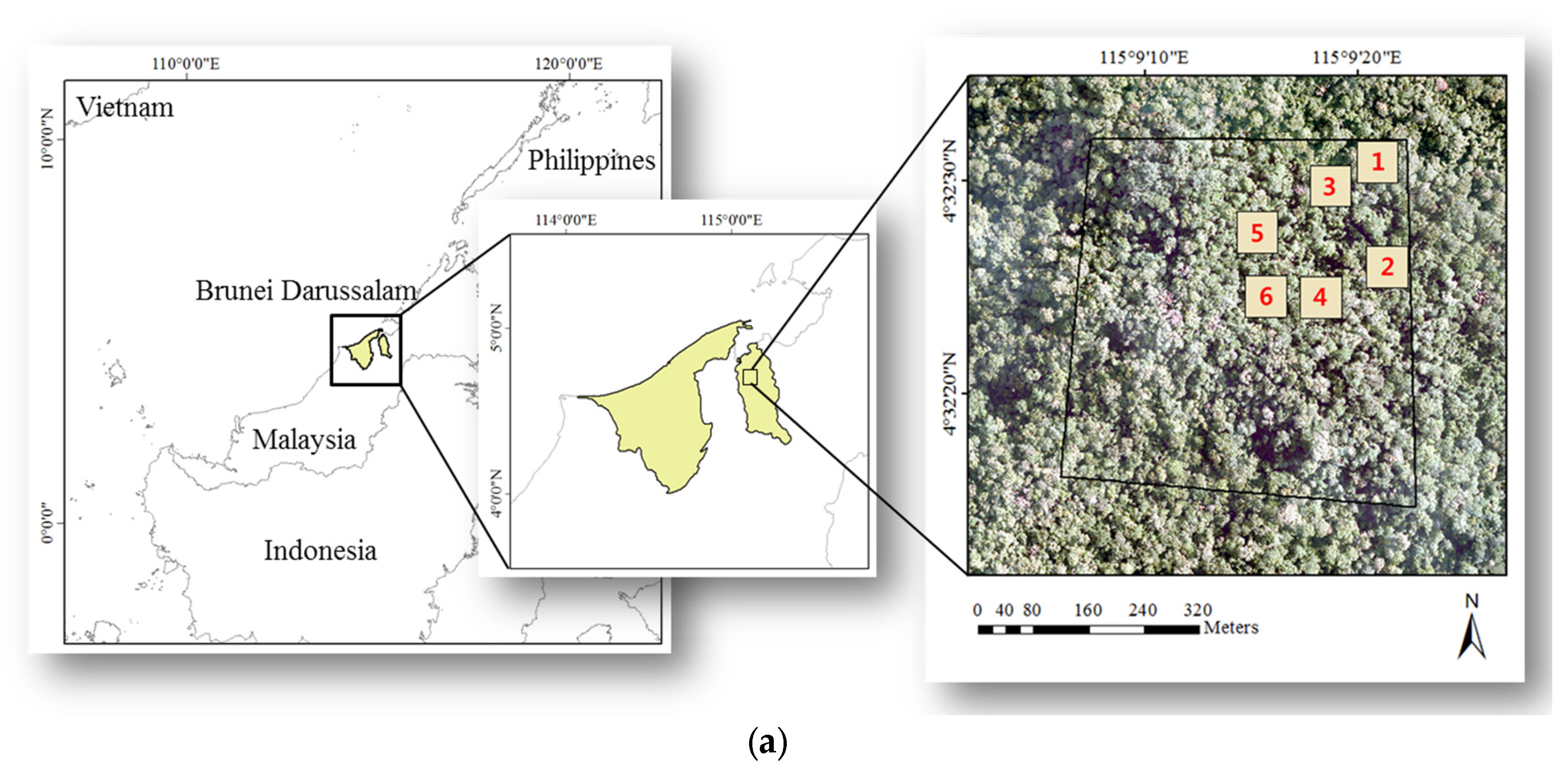
2.1. Study Area

The study area was located in the Kuala Belalong Field Studies Centre (KBFSC; 04°32′50.1″ N, 115°09′29.6″ E) in the Ulu Temburong National Park, Brunei Darussalam. The KBFSC is 25 ha of intact tropical rain forest, which consists of lowland mixed dipterocarp forest (MDF), at an elevation range of 49 m to 307 m above sea level. Meteorological data for the study area were obtained from the Semabat area of Semabat Agricultural Station, which is 9 km west-northwest of the KBFSC. These data were analyzed by collecting climate data from 2007 to 2010 and rainfall data from 2006 to 2010 [9,13,24]. The daily maximum temperature ranged from 30.58 °C to 35.08 °C and the daily minimum temperature ranged from 25.6 °C to 26.2 °C. The average annual rainfall during the study period was 4582 mm, with 240 rain days per year. The spatial pattern of the rainfall was heavily concentrated in a small area over a short period of time [30]. While small and young understory trees had a monopodial crown shape, mature trees had a sympodial crown shape in which the crown width is broader than its height [10,31].
Researchers at the Center for Tropical Forest Science (CTFS) and University of Brunei Darussalam (UBD) established 25 ha of forest dynamics plots for the field study of carbon stock estimation and carbon sequestration, and have monitored the area since 2011 (Figure 1a). Field inventory data for six 60 m × 60 m plots, located in the northeastern part of the forest dynamics plot, were provided by UBD at a horizontal collection interval of 10 m. We subdivided the plots further into 20 m × 20 m and 30 m × 30 m for the estimation of AGB (Figure 1b), for a total of fifty-four 20 m × 20 m plots and twenty-four 30 m × 30 m plots (Figure 1b).
Field inventory data were obtained in 2011 from the CTFS. Data on diameter at breast height (DBH) over 1 cm and the relative position of individual trees in each plot were collected. DBH of individual trees was less than 10 cm in 91% of the study area. Above-ground biomass (AGB) was calculated from trees whose DBH was ≥1 according to the allometric equation, and plot-level AGB of the study area was estimated by summing the number of individual trees located in each plot. The allometric equation was developed in lowland dipterocarp forests by Basuki et al. ([32], Equation (1)).
ln ( TAGB ) = 1.232 + 2.178 × ln ( DBH )
where TAGB is the total above-ground biomass measured in kg/tree and DBH is measured in cm.
The number of individual trees with DBH < 10 cm occupied 91% of the total area and yet their AGB contributed only 8.47% of the total biomass in the 2.16 ha area. In contrast, trees with DBH > 10 cm occupied only 9% of the study site and yet their AGB corresponded to 91.53% of the total biomass in the area (Table 1). To reduce the influence of edge effects, plot-level AGB for 20 m × 20 m and 30 m × 30 m plots was calculated. The edge effect determines that as the size of plot becomes smaller, big trees have greater influence and result in a higher standard deviation (SD). Supporting this theoretical knowledge, the average AGB ± SD of the 20 m and 30 m plots were 313.75 ± 150.81 Mg∙ha−1 and 302.71 ± 98.51 Mg∙ha−1, respectively. Additionally, 20 m plots were characterized by a significantly greater variation in each plot compared with the 30 m plots.

2.2. Airborne LiDAR Data
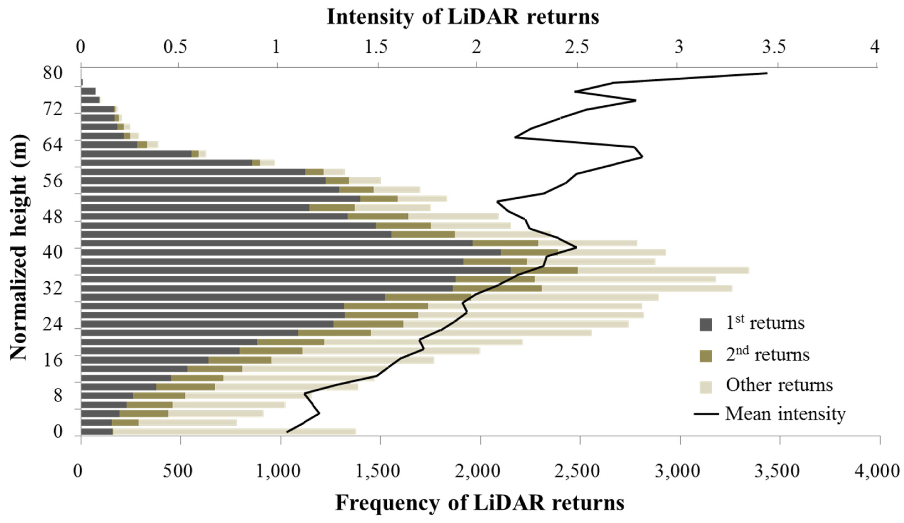
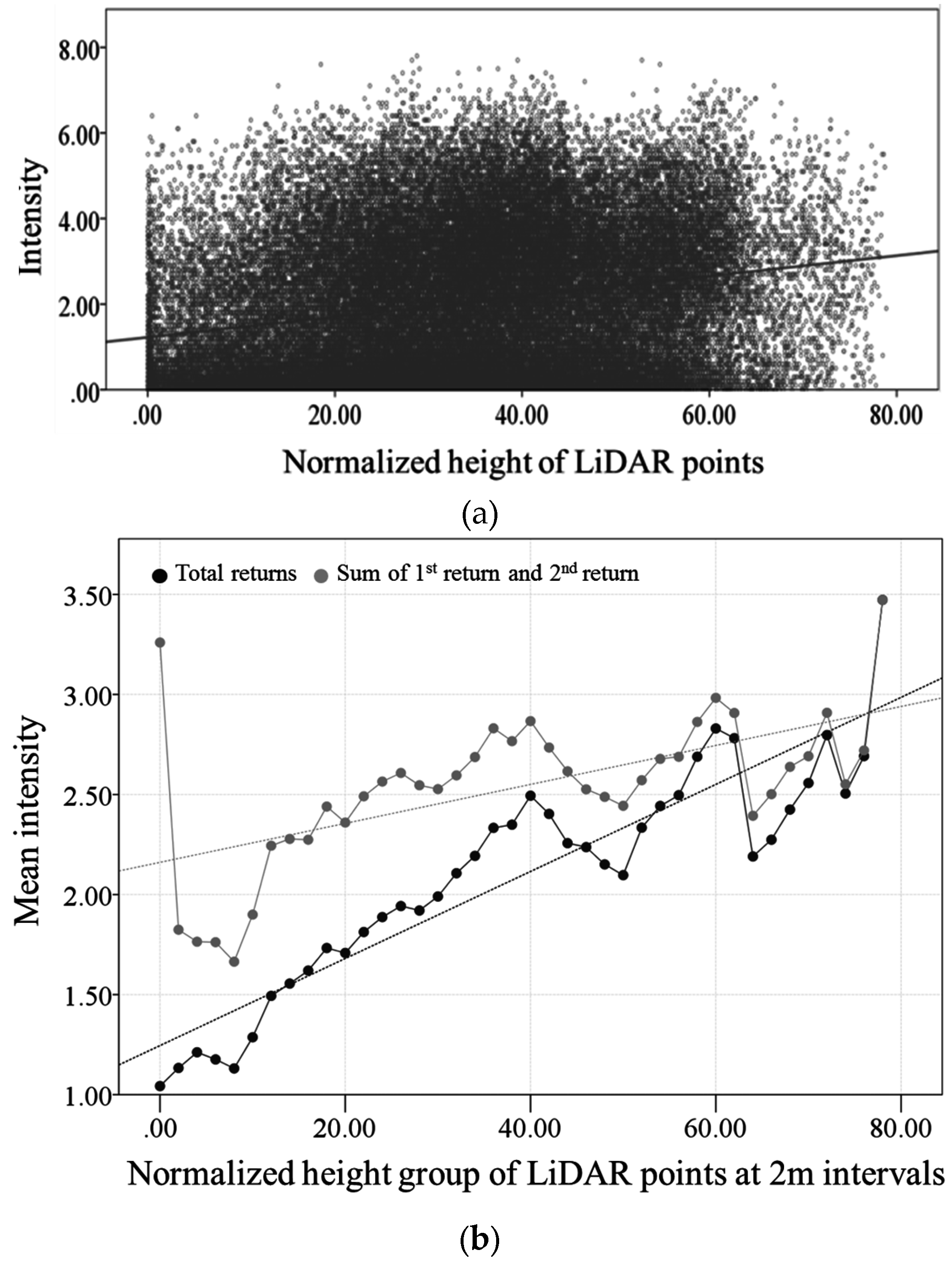
Airborne LiDAR data were acquired at an average of 1400 m above ground level (AGL) in April 2009 with a sampling density of 1.13 pt∙m−2 (Figure 2). LiDAR acquisition was conducted with a laser footprint on the ground of 34 cm and a scan angle of ± 20° at the rate of 35 Hz. The LiDAR system recorded four returns from a single laser pulse; 1st return, intermediate return 1 (2nd), intermediate return 2 (3rd), and last return (4th). Each return contained X, Y, Z, and intensity values.
For the normalization of the raw LiDAR point cloud data, the normalized height, referring to the Z value of terrain, was calculated (Figure 2). First, a digital terrain model (DTM) was generated from last returns using a triangulated irregular network (TIN) interpolation method at a spatial resolution of 1 m [19]. Second, the normalized height values were determined as the height difference between each raw LiDAR point and its corresponding DTM value [10,33,34]. Last, abnormal values such as NULL values and negative height values were removed.

2.3. LiDAR Metrics

Full usage of LiDAR point cloud data allows a more sophisticated and detailed approach, unlike CHM based analysis. Typical examples of full usage are LiDAR height and intensity distributional metrics and statistics such as percentile, maximum height, minimum height, and intensity. Additionally, the volumetric pixel (voxel), implemented in this study, is a comprehensive approach that illustrates both vertical and horizontal slices of LiDAR point cloud data. This study used both point cloud-based (PCB) and voxel-based (VB) metrics to gain a better understanding of the 3-D forest structure in the multi-layered forest of the KBFSC study area (Table 2). In total, 118 LiDAR metrics were derived from the 20 m × 20 m plots and 30 m × 30 m plots.

2.4. Point Cloud Based (PCB) LiDAR Metrics

LiDAR height and intensity distributional parameters were built using the normalized LiDAR point cloud height and intensity values of each point. These were treated as independent variables, which are the explanatory variables for estimating plot-level AGB. A total of 29 variables were classified into three data sets for interpreting the vertical height profile of each plot: (1) height data set; (2) intensity data set; and (3) ratio metrics data set [23,33,35]. These variables were recorded at 10 percentile intervals from 0 to 100 percentile height (HP10, HP20, …, HP100), for the purpose of defining the relationship between AGB and height [36]. In addition, maximum, minimum, average, and median statistics of height and intensity values were also examined. A more detailed description of the variables is presented in Table 2.

2.5. Voxel-Based (VB) Metrics

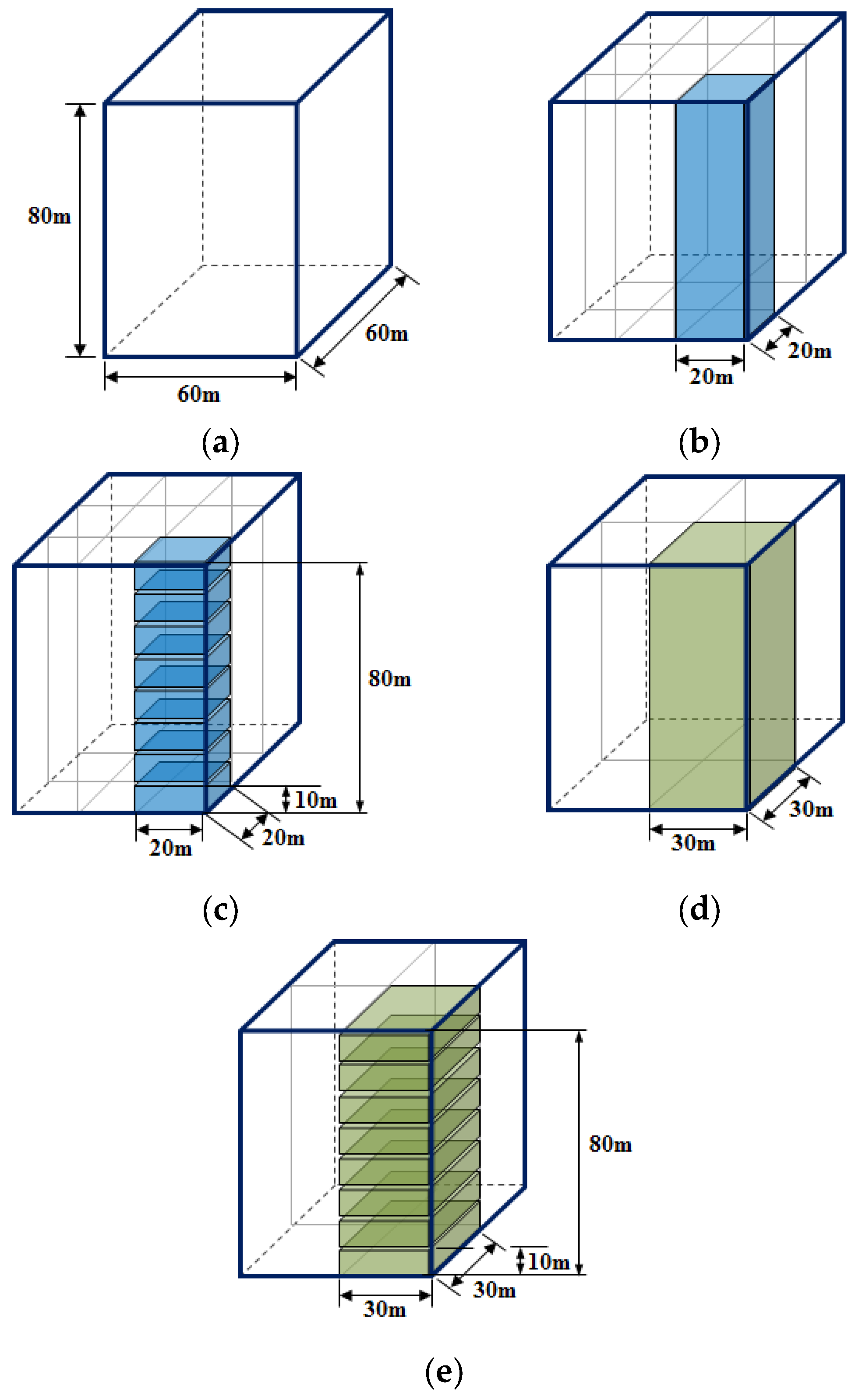
2.5.1. Extraction of LiDAR Point Cloud Data Based on the Voxel Approach

Unless using CHM analysis, full usage of LiDAR points is difficult to achieve due to the massive quantity of points. To solve this issue, we developed an algorithm in this study to conduct a time-efficient voxel-based approach analysis in RStudio (R version 3.2.3). Voxels in the form of a regular 3-D grid (similar to a 3-D cube) were created at a pre-defined horizontal and vertical resolution. In accordance with a pre-defined plot size (60 m × 60 m) for field measurements, the X, Y values were set as 60 m × 60 m and the Z value was set to the maximum LiDAR point height, 80 m (Figure 3a). X, Y values were then subdivided into both 20 m × 10 m and 30 m × 30 m intervals (Figure 3b,d) and the Z value was subdivided into user-defined 10 m vertical intervals (Figure 3c,e).
Finally, the voxel-based LiDAR metrics were computed based on the LiDAR points within each sub-voxel (SV). From this point forward, each SV that was divided into 10-m vertical intervals is referred to as SV1 (0–10 m), …, SV7 (60–70 m), SV8 (70–80 m) (Figure 3c,e).

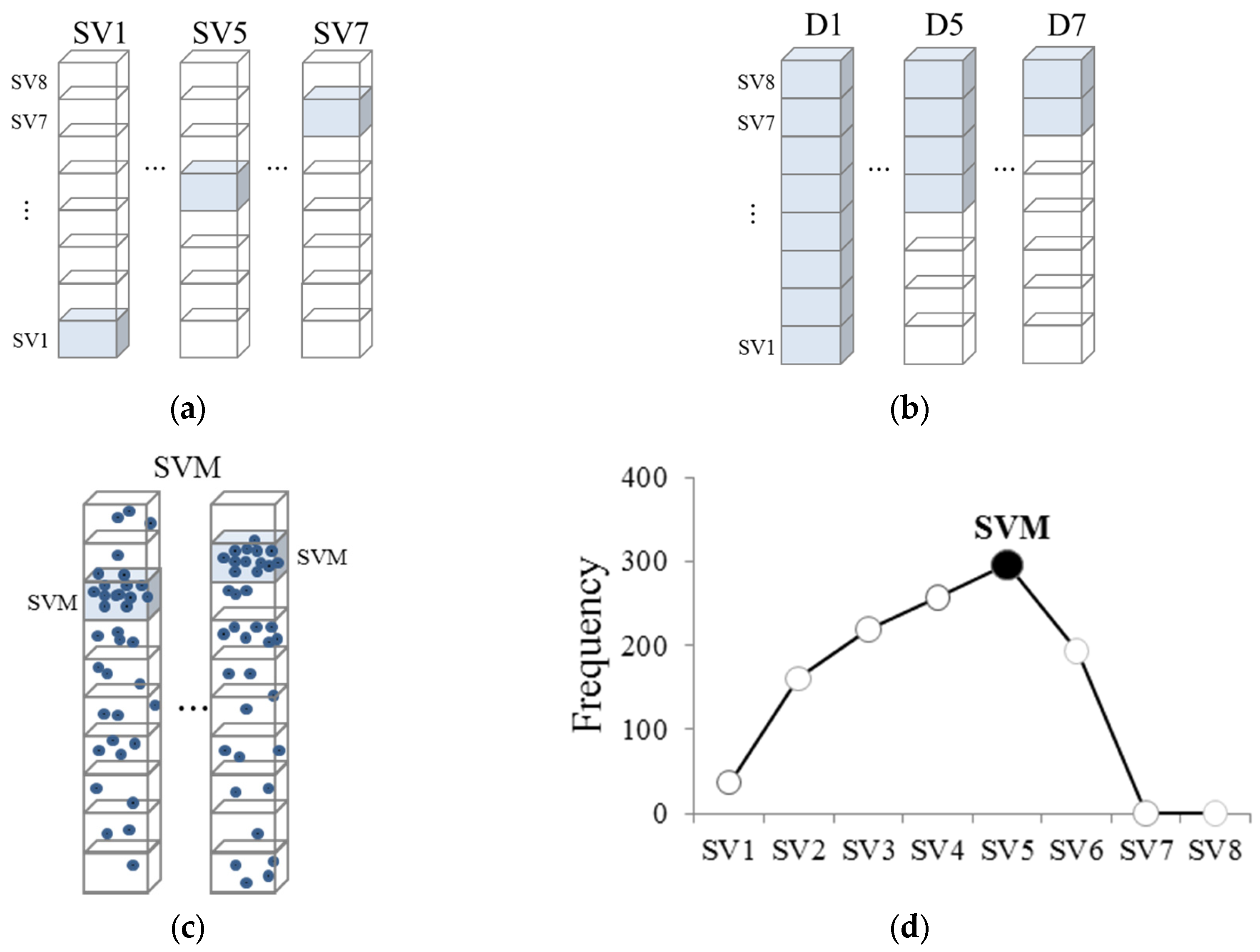
2.5.2. Concepts of Voxel-Based (VB) Metrics

The voxel-based LiDAR metrics employed in this study can be divided into three basic variable concepts as follows; Variable Sub-Voxel i (SVi), Variable Density i (Di), Variable Sub-Voxel Maximum (SVM) (Figure 4a–c). Sheridan et al. [27] proposed the concepts of Variable SVi and Variable Di, and a new variable approach of Variable SVM was added in this study. Using these three concepts for building VB metrics, a number of points, frequency ratios, median intensities, and median height values were calculated (Table 2). To find out how dense the corresponding voxel was compared to all returns, the frequency ratio variable was calculated as the fraction of total LiDAR points versus the points that existed within or above SVi. Variable SVi accounted for the variables derived from the points in their corresponding SV (Figure 4a). For example, P_SV5 represented the total LiDAR returns within SV5, ranging from 40 m to 50 m. In contrast, Variable Di described the cumulative points located above the corresponding SV (Figure 4b). For example, I_D5med represented the median intensity of accumulative LiDAR points above SV5, ranging from 40 m to 80 m. Variable SVM was the location of the greatest point density, where the highest frequency of LiDAR returns occurred within the entire range of SV1 to SV8 (Figure 4c,d). After locating SVM, the points within (SVi) or above (Di) SVM were extracted and used for building further variables. For example, H_SVMmed represented the median height of SV, which exhibited the highest point density throughout SV1 to SV8.
Intermediate return is expected to have high applicability in dealing with multi-layered forests, such as tropical rain forests, because these returns have the ability to reflect mid-canopy forest structure [12]. However, only a few studies have attempted to incorporate intermediate returns (2nd, 3rd returns) on a deeper level [37]. In this study, 2nd returns were added to the database of the 1st and last returns in hopes of increasing the accuracy of the analysis and obtaining a better understanding of the multi-layered forest. For various purposes, all variables were extracted using either total LiDAR returns, first returns only (e.g., for P_DiF), and the sum of 1st and 2nd returns (e.g., for P_DiFS).

2.6. Statistical Analysis

To predict plot-level AGB using LiDAR data, a multiple linear regression analysis (Equation (2); [23]) was performed with a stepwise selection method at a significance level of 0.05 with ten or less predictors as a result.
y = α + β 1 x 1 + β 2 x 2 + + β n x n + ε
where AGB is the plot-level AGB in Mg∙ha−1; x1, x2, …, xn are the selected LiDAR variables as predictors; α is the intercept of the regression; β1, β2, …, βn are the slope coefficients of the regression; and ε is the residual.
Multiple regression analysis was applied separately to the 20 m × 20 m plot and the 30 m × 30 m plot. To determine the optimal model for each by plot size, the statistics coefficient of determination (R2), adjusted coefficient of determination (Adj. R2) and standard error (SE) were calculated for each model using RStudio (R version 3.2.3, RStudio, Inc., Boston, MA, USA) and compared. Furthermore, to avoid multicollinearity among independent variables, a variance inflation factor (VIF) of less than 10 was required for selection as an independent variable [23,27]. To avoid inaccuracies from an excessive number of the predictors, the total number of selected independent variables was limited to 10. Predicted models from multiple regression analyses were validated using root-mean-square error (RMSE) and normalized root-mean-square error in percentage (NRMSE%). RMSE indicates the absolute value of error, whereas NRMSE% is the ratio of RMSE versus the average value of the dependent variables ( y ¯ ) and thus represents the relative value of the error with respect to the average plot-level AGB (Equations (3) and (4)).
RMSE ( Mg · h a 1 ) = i = 1 n ( y o b s e r v e d y p r e d i c t e d ) 2 n
NRMSE ( % ) = R M S E y ¯ × 100
where yobserved is the plot-level field AGB in Mg∙ha−1, ypredicted is the LiDAR-estimated plot-level AGB in Mg∙ha−1, and y ¯ is the average value of plot-level field AGB in Mg∙ha−1.

3. Results and Discussion

3.1. Development of Models for AGB Estimation

Multiple linear regression analysis for each plot size was performed to predict plot-level AGB at a significance level of 0.05. In total, 118 LiDAR metrics combining point cloud based (PCB) metrics and voxel-based (VB) metrics were used for developing and assessing the accuracy of the regression models The R2, Adj. R2, and SE values of the 20 m × 20 m plot model (n = 54) were 0.72, 0.69, and 107.56 Mg∙ha−1, respectively (Table 3). Four independent variables were selected, including one variable from PCB metrics and three variables from VB metrics. The R2, Adj. R2, and SE values of the 30 m × 30 m plots model (n = 24) were 0.92, 0.87, and 35.13 Mg∙ha−1, respectively. The model defined for both scenarios selected more independent variables from VB metrics than from PCB metrics. It is postulated that VB metrics held more power than PCB metrics in explaining AGB in stratum-specific analysis because its variables were produced from points at various height layers, whereas the PCB metrics did not implement height stratification (Table 3).
The coefficients of all selected independent variables were interpreted. Since the coefficients for variables P_SV1, HP10, HP20, and FR_SV1 were negative, it is understood that AGB tends to increase with the number of points in the understory layer of 0 to 20 m. This indicates that in plots where the emergent and canopy layer are dominant, the growth of understory vegetation is hindered because less than 2%–15% of sunlight can reach the ground. On the other hand, plots with less understory vegetation can also be interpreted as having a prevalence of large trees. In this respect, it is determined that the variables representing understory layer have a negative relationship with plot AGB.
Variable “H_SVMmed” was notable as it was selected in both 20 m × 20 m and 30 m × 30 m plot models. This variable is comprised of median height values from SVM, which had the highest point density among SV1 to SV8 (0–80 m). This indicates the greater the elevation of the densest forest layer, the higher its explanatory power of AGB.
Intensity values have often been used for species classification and are one of the key factors used in understanding forest biophysical parameters [23,38,39,40,41,42]. Six intensity related variables were also adopted in this study. VB intensity variables I_SV2med_FS, I_SV3med, I_SV3med_FS, and I_D8med and PCB intensity variables IRange and IStd were selected as the predictors of the regression models. The mean intensity value of points was calculated at 2-m intervals between the heights of 0 m and 80 m, and it was observed that intensity value tended to increase with canopy height (Figure 5a) with a high correlation between height group and mean intensity (Figure 5b). This finding indicates that intensity-related variables and height values of LiDAR points can be representative descriptors of plot AGB.

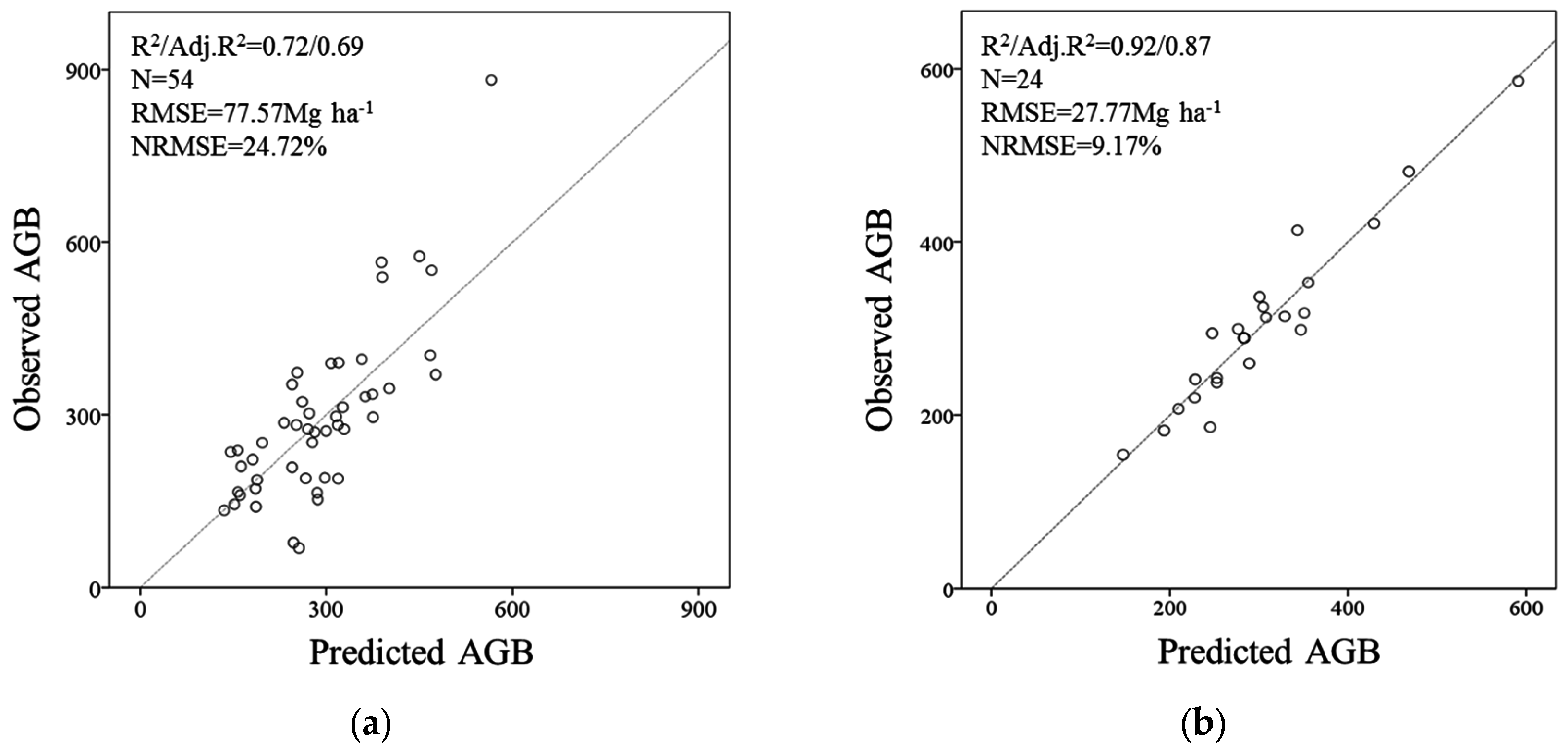
3.2. Statistical Analysis for Model Validation

AGB values predicted using the regression model were assessed for accuracy using field-measured AGB (observed AGB) data (Table 4; Figure 6). To validate the model accuracy, values of RMSE (Mg∙ha−1) and NRMSE% were examined. Model validation for the 20 × 20 m plots yielded RMSE and NRMSE values of 77.57 Mg∙ha−1 and 24.72%, respectively. Observed AGB was 313.75 ± 150.81 Mg∙ha−1, while the LiDAR model under-estimated AGB at 290.85 ± 98.16 Mg∙ha−1. Model validation for the 30 × 30 m plot yielded RMSE and NRMSE% values of 27.77 Mg∙ha−1 and 9.17%, respectively. Observed and predicted AGB in the 30-m plots showed a high level of agreement, as demonstrated by the same average AGB value of 302.71 Mg∙ha−1. The discrepancy in accuracy between the 20-m and 30-m plot AGB predictions may have been caused by the differing sample size available (20-m plots n = 54 and 30-m plots n = 24). However, since the field inventory data indicated that the SE value of the 20-m plots (150.81 Mg∙ha−1) was greater than the 30-m plots (94.33 Mg∙ha−1), it was determined that the smaller plot size is more highly influenced by edge effects. Accordingly, the 30 m × 30 m plots were determined to be more reliable for research purposes than 20 m × 20 m plots in this study area.
Very few studies have focused on high-biomass forests with average AGB over 200 Mg∙ha−1 [3,4,43,44,45]. High-biomass forests such as those found in the tropics could have a significant bias in AGB estimation owing to greater absolute error caused by their more complicated structure relative to other forest types (biomes). To verify how well our high-biomass AGB prediction models performed, we compared our results with those of previous airborne LiDAR studies that were conducted in high-biomass forests (>200 Mg∙ha−1) on 30 m × 30 m plots (Table 5). For quantitative evaluation, average AGB (Mg∙ha−1), LiDAR point density (pts∙m−2), RMSE (Mg∙ha−1), and NRMSE% were reviewed. Overall LiDAR point density of the comparison studies was 2–25 times higher than that used in this study and their average field AGB was 235.5 to 461.9 Mg∙ha−1.
Phua et al. [4] performed a PCB approach on a logged tropical rain forest in Malaysia, close to our study area in Borneo. Their study area was also lowland MDF, akin to our study. They created height percentile variables as predictors and derived R2 and NRMSE values of 0.67% and 22.3%, respectively. Thus the current study yielded higher confidence performance despite a 25-fold lesser LiDAR point density. Ioki et al. [43] also estimated plot-level AGB in Borneo, Malaysia, in the transition zone between lowland and mountain forests through the combined use of mean CHM value and height percentiles derived from the point cloud basis. Their average AGB was 235.5 Mg∙ha−1, which is a relatively lower level than that found in this study. The values of Adj. R2 and NRMSE were 0.81% and 26.0%, respectively. Mauya et al. [3] used the PCB approach for their analysis with optimal plot size in the tropical rain forest of Tanzania. This study concluded with an NRMSE value of 29.2% at the plot size of 2000 m2, with a high LiDAR point density of 10.6 pts∙m−2. Additionally, the study area of Hansen et al. [44] had a considerably high AGB of 461.9 Mg∙ha−1, determined using a PCB approach to describe height and density of the forest canopy for R2 and NRMSE values of 0.71% and 34.4%, respectively. Lastly, Lu et al. [45] predicted an average field AGB of 239.1 Mg∙ha−1 in a temperate rain forest within the USA. The R2 value was 0.76, but NRMSE was relatively high at 34.4%, and LiDAR point density was a low 2 pts∙m−2.
The current study is notable in that it efficiently analyzed the complicated intact tropical rain forest with a high accuracy using the new approach. The lowland MDF of this study area contains a morphologically different crown shape according to the age of each tree. Small and young understory trees have a monopodial crown shape, while mature trees have a sympodial crown shape with a broader crown width than crown height [10,31]. Furthermore, the characteristics of the tropical rain forest, especially ‘intact’ rainforest are more complex and multi-layered than other forests, with different structural objects and a high stand density. The current study implemented a very low LiDAR density (1 pt∙m−2) compared to previous research, which ranged from 2 to 25 pts∙m−2. Nevertheless, the AGB prediction models developed in this study showed more accurate results than previous studies.

4. Conclusions

The present study aimed to estimate plot-level AGB and to develop a regression model through a voxel-based approach using airborne LiDAR data from an intact tropical rain forest. The comprehensive volumetric pixel (voxel) approach illustrated both vertical and horizontal slices of LiDAR point cloud data in the form of a 3-D cube, and was expected to sufficiently represent the structural complexity of the forest.
By using both point cloud-based (PCB) metrics and voxel-based (VB) metrics, we were able to promote the advantages of LiDAR data, which are able to describe 3-D forest structures with 3-D point cloud data. After calculating plot-level field AGB from DBH data of individual trees at two different plot sizes of 20 m × 20 m and 30 m × 30 m, multiple linear regression analyses were performed to derive the best models for estimating AGB at each plot size. The results of regression analysis indicated that the 30 m × 30 m plot model was more accurate in predicting AGB than the 20 m × 20 m plot model, with R2, adj. R2, and SE values of 0.92, 0.87, and 35.13 Mg∙ha−1, respectively. Both 20 m × 20 m and 30 m × 30 m models selected a greater number of independent variables from VB metrics than from PCB metrics. It is postulated that VB metrics were selected because their stratum-specific AGB quantification of AGB provides greater power in AGB prediction. PCB metrics do not have this advantage because they are not derived from points located in specific height layers. We therefore expect the VB metrics to be more applicable in tropical rain forests where multi-layer structured vegetation is prevalent.
Comparing predicted and observed AGB for model validation, the value of RMSE was 27.8 Mg∙ha−1. To relate the value of RMSE to the average field value of AGB, NRMSE% was calculated as 9.2%. This study provides a high confidence estimate for complicated intact tropical rain forest, relative to those found in previous research (NRMSE% from 22.3% to 34.4%), even though the density of our LiDAR returns was low. This new voxel-based approach is expected to contribute to the advancement of forest carbon quantification techniques. However, this study is limited in that it is constrained to an intact MDF forest in a tropical region within a relatively small number of 24 sample plots. This research can be furthered by applying the same techniques in other forest climatic zones (e.g., the temperate forests of Korea) to examine their effectiveness more broadly.

Acknowledgments

This research was supported by the Korea Forest Service (Grant number S121314L130120).

Author Contributions

All of the authors contributed the overall research design. The main author analyzed the data and wrote the early drafts of this manuscript. The others provided comment for the edits.

Conflicts of Interest

The authors declare no conflict of interest.

References

  1. FAO (Food and Agriculture Organization of the United Nations). Global Forest Resources Assessment 2010 Main Report; Food and Agriculture Organization of the United Nations: Rome, Italy, 2010. [Google Scholar]
  2. Pachauri, R.K.; Allen, M.R.; Barros, V.R.; Broome, J.; Cramer, W.; Christ, R.; Church, J.A.; Clarke, L.; Dahe, Q.; Dasgupta, P.; et al. Contribution of working groups I, II and III to the fifth assessment report of the intergovernmental panel on climate change. In Climate Change 2014: Synthesis Report; Intergovernmental Panel on Climate Change: Bonn, Germany, 2014; p. 151. [Google Scholar]
  3. Mauya, E.W.; Hansen, E.H.; Gobakken, T.; Bollandsås, O.M.; Malimbwi, R.E.; Næsset, E. Effects of field plot size on prediction accuracy of aboveground biomass in airborne laser scanning-assisted inventories in tropical rain forests of Tanzania. Carbon Bal. Manag. 2015, 10, 1–14. [Google Scholar] [CrossRef] [PubMed] [Green Version]
  4. Phua, M.H.; Hue, S.W.; Loki, K.; Hashim, M.; Bidin, K.; Musta, B.; Suleiman, M.; Yap, S.W.; Maycock, C.R. Estimating aboveground biomass of a logged-over lowland rainforest in Sabah, Malaysia using airborne LiDAR data. Terr. Atmos. Ocean Sci. 2016, in press. [Google Scholar] [CrossRef]
  5. Réjou-Méchain, M.; Tymen, B.; Blanc, L.; Fauset, S.; Feldpausch, T.R.; Monteagudo, A.; Phillips, O.L.; Richard, H.; Chave, J. Using repeated small-footprint LiDAR acquisitions to infer spatial and temporal variations of a high-biomass Neotropical forest. Remote Sens. Environ. 2015, 169, 93–101. [Google Scholar] [CrossRef] [Green Version]
  6. Huntingford, C.; Zelazowski, P.; Galbraith, D.; Mercado, L.M.; Sitch, S.; Fisher, R.; Lomas, M.; Walker, A.P.; Jones, C.D.; Booth, B.B.; et al. Simulated resilience of tropical rainforests to CO2-induced climate change. Nat. Geosci. 2013, 6, 268–273. [Google Scholar] [CrossRef]
  7. Gumpenberger, M.; Vohland, K.; Heyder, U.; Poulter, B.; Macey, K.; Rammig, A.; Popp, A.; Cramer, W. Predicting pan-tropical climate change induced forest stock gains and losses—Implications for REDD. Environ. Res. Lett. 2010, 5, 1–15. [Google Scholar] [CrossRef]
  8. Cox, P.M.; Pearson, D.; Booth, B.B.; Friedlingstein, P.; Huntingford, C.; Jones, C.D.; Luke, C.M. Sensitivity of tropical carbon to climate change constrained by carbon dioxide variability. Nature 2013, 494, 341–344. [Google Scholar] [CrossRef] [PubMed]
  9. Lee, S.; Lee, D.; Yoon, T.K.; Salim, K.A.; Han, S.; Yun, H.M.; Yoon, M.; Kim, E.; Lee, W.K.; Davies, S.J.; et al. Carbon stocks and its variations with topography in an intact lowland mixed dipterocarp forest in Brunei. J. Ecol. Environ. 2015, 38, 75–84. [Google Scholar] [CrossRef]
  10. Kim, E.; Lee, W.K.; Yoon, M.; Lee, J.Y.; Lee, E.J.; Moon, J.Y. Detecting individual tree position and height using Airborne LiDAR data in Chollipo Arboretum, South Korea. Terr. Atmos. Ocean Sci. 2016. in Press. [Google Scholar] [CrossRef]
  11. Cui, G.S.; Lee, W.K.; Zhu, W.H.; Lee, J.; Kwak, H.; Choi, S.; Kwak, D.A.; Park, T. Vegetation classification and biomass estimation using IKONOS imagery in Mt. ChangBai mountain area. J. Korean For. Soc. 2012, 101, 356–364. [Google Scholar]
  12. Van Aardt, J.A.; Wynne, R.H.; Scrivani, J.A. Lidar-based mapping of forest volume and biomass by taxonomic group using structurally homogenous segments. Photogramm. Eng. Remote Sens. 2008, 74, 1033–1044. [Google Scholar] [CrossRef]
  13. Yoon, M.; Kim, E.; Kwak, D.A.; Lee, W.K.; Lee, J.Y.; Kim, M.I.; Lee, S.; Son, Y.; Salim, K.A. Estimation of stand-level above-ground biomass in intact tropical rain forests of Brunei using airborne LiDAR data. Korean J. Remote Sens. 2015, 31, 127–136. [Google Scholar] [CrossRef]
  14. Lang, M.W.; McCarty, G.W. LiDAR Intensity for Improved Detection of Inundation below the Forest Canopy. Wetlands 2009, 29, 1166–1178. [Google Scholar] [CrossRef]
  15. Ruiz, L.A.; Hermosilla, T.; Mauro, F.; Godino, M. Analysis of the influence of plot size and LiDAR density on forest structure attribute estimates. Forests 2014, 5, 936–951. [Google Scholar] [CrossRef]
  16. Frazer, G.W.; Magnussen, S.; Wulder, M.A.; Niemann, K.O. Simulated impact of sample plot size and co-registration error on the accuracy and uncertainty of LiDAR-derived estimates of forest stand biomass. Remote Sens. Environ. 2011, 115, 636–649. [Google Scholar] [CrossRef]
  17. Mascaro, J.; Detto, M.; Asner, G.P.; Muller-Landau, H.C. Evaluating uncertainty in mapping forest carbon with airborne LiDAR. Remote Sens. Environ. 2011, 115, 3770–3774. [Google Scholar] [CrossRef]
  18. Næsset, E.; Bollandsås, O.M.; Gobakken, T.; Gregoire, T.G.; Ståhl, G. Model-assisted estimation of change in forest biomass over an 11-year period in a sample survey supported by airborne LiDAR: A case study with post-stratification to provide ‘activity data’. Remote Sens. Environ. 2013, 128, 299–314. [Google Scholar] [CrossRef]
  19. Kim, E.M. Extraction of the tree regions in forest areas using LiDAR data and ortho-image. J. Korean Soc. Geospat. Inform. Syst. 2013, 21, 27–34. [Google Scholar] [CrossRef]
  20. Yunfei, B.; Guoping, L.; Chunxiang, C.; Xiaowen, L.; Hao, Z.; Qisheng, H.; Linyan, B.; Chaoyi, C. Classification of LIDAR point cloud and generation of DTM from LIDAR height and intensity data in forested area. Int. Arch. Photogramm. Remote Sens. Spat. Inform. Sci. 2008, 37, 313–318. [Google Scholar]
  21. El-Ashmawy, N.; Shaker, A. Raster vs. point cloud LiDAR data classification. Int. Arch. Photogramm. Remote Sens. Spat. Inform. Sci. 2014, 40, 79. [Google Scholar] [CrossRef]
  22. Hagstrom, S.T. Voxel-Based LIDAR Analysis and Applications. Ph.D. Thesis, Rochester Institute of Technology, New York, NY, USA, 2014. [Google Scholar]
  23. Kwak, D.A.; Cui, G.; Lee, W.K.; Cho, H.K.; Jeon, S.W.; Lee, S.H. Estimating plot volume using LiDAR height and intensity distributional parameters. Int. J. Remote Sens. 2014, 35, 4601–4629. [Google Scholar] [CrossRef]
  24. Yoon, M.; Kim, E.; Lee, W.K.; Kim, M.I.; Lee, S.; Son, Y.; Salim, K.A. Estimating above-ground biomass in intact tropical forest of Brunei using LiDAR data according to plot size. Adv. Space Res. 2016. submitted. [Google Scholar]
  25. Mutlu, M.; Popescu, S. Assessing forest fuel models using LiDAR remote sensing. In Proceedings of the ASPRS 2006 Annual Conference, Reno, NV, USA, 1–5 May 2006.
  26. Popescu, S.C.; Zhao, K. A voxel-based Lidar method for estimating crown base height for deciduous and pine trees. Remote Sens. Environ. 2008, 112, 767–781. [Google Scholar] [CrossRef]
  27. Sheridan, R.D.; Popescu, S.C.; GatSViolis, D.; Morgan, C.L.; Ku, N.W. Modeling forest aboveground biomass and volume using airborne LiDAR metrics and forest inventory and analysis data in the Pacific Northwest. Remote Sens. 2014, 7, 229–255. [Google Scholar] [CrossRef]
  28. Zhao, K.; Popescu, S.; Nelson, R. LiDAR remote sensing of forest biomass: A scale-invariant estimation approach using airborne lasers. Remote Sens. Environ. 2009, 113, 182–196. [Google Scholar] [CrossRef]
  29. Vetter, M.; Höfle, B.; Hollaus, M.; Gschöpf, C.; Mandlburger, G.; Pfeifer, N.; Wagner, W. Vertical vegetation structure analysis and hydraulic roughness determination using dense ALS point cloud data—A voxel based approach. Int. Arch. Photogramm. Remote Sens. Spat. Inform. Sci. 2011, 38, 5. [Google Scholar] [CrossRef]
  30. Dykes, A.P. Climatic patterns in a tropical rainforest in Brunei. Geogr. J. 2000, 166, 63–80. [Google Scholar] [CrossRef]
  31. Kricher, J. Tropical Ecology; Princeton University Press: Princeton, NJ, USA, 2011. [Google Scholar]
  32. Basuki, T.M.; Van Laake, P.E.; Skidmore, A.K.; Hussin, Y.A. Allometric equations for estimating the above-ground biomass in tropical lowland Dipterocarp forests. For. Ecol. Manag. 2009, 257, 1684–1694. [Google Scholar] [CrossRef]
  33. Kwak, D.A.; Lee, W.K.; Cho, H.K.; Lee, S.H.; Son, Y.; Kafatos, M.; Kim, S.R. Estimating stem volume and biomass of Pinus koraiensis using LiDAR data. J. Plant Res. 2010, 123, 421–432. [Google Scholar] [CrossRef] [PubMed]
  34. Wang, Y.; Weinacker, H.; Koch, B. A LiDAR point cloud based procedure for vertical canopy structure analysis and 3-D single tree modelling in forest. Sensors 2008, 8, 3938–3951. [Google Scholar] [CrossRef]
  35. Clark, M.L.; Roberts, D.A.; Ewel, J.J.; Clark, D.B. Estimation of tropical rain forest aboveground biomass with small-footprint LiDAR and hyperspectral sensors. Remote Sens. Environ. 2011, 115, 2931–2942. [Google Scholar] [CrossRef]
  36. García, M.; Riaño, D.; Chuvieco, E.; Danson, F.M. Estimating biomass carbon stocks for a Mediterranean forest in central Spain using LiDAR height and intensity data. Remote Sens. Environ. 2010, 114, 816–830. [Google Scholar] [CrossRef]
  37. Shendryk, I.; Hellström, M.; Klemedtsson, L.; Kljun, N. Low-density LiDAR and optical imagery for biomass estimation over boreal forest in Sweden. Forests 2014, 5, 992–1010. [Google Scholar] [CrossRef]
  38. Cao, L.; Coops, N.C.; Hermosilla, T.; Innes, J.; Dai, J.; She, G. Using small-footprint discrete and full-waveform airborne LiDAR metrics to estimate total biomass and biomass components in subtropical forests. Remote Sens. 2014, 6, 7110–7135. [Google Scholar] [CrossRef]
  39. Martin, M.E.; Newman, S.D.; Aber, J.D.; Congalton, R.G. Determining forest species composition using high spectral resolution remote sensing data. Remote Sens. Environ. 1998, 65, 249–254. [Google Scholar] [CrossRef]
  40. Fung, T.; Fung Yan Ma, H.; Siu, W.L.; Lin, H.; Gong, P. Subtropical tree recognition with hyperspectral data analysis in Hong Kong. Geocarto Int. 2001, 16, 25–34. [Google Scholar] [CrossRef]
  41. Van Aardt, J.A.N.; Wynne, R.H. Spectral Separability among six southern tree species. Photogramm. Eng. Remote Sens. 2001, 67, 1367–1375. [Google Scholar]
  42. Ørka, H.O.; Gobakken, T.; Næsset, E.; Ene, L.; Lien, V. Simultaneously acquired airborne laser scanning and multispectral imagery for individual tree species identification. Can. J. Remote Sens. 2012, 38, 125–138. [Google Scholar] [CrossRef]
  43. Ioki, K.; Tsuyuki, S.; Hirata, Y.; Phua, M.H.; Wong, W.V.C.; Ling, Z.Y.; Saito, H.; Takao, G. Estimating above-ground biomass of tropical rainforest of different degradation levels in Northern Borneo using airborne LiDAR. For. Ecol. Manag. 2014, 328, 335–341. [Google Scholar] [CrossRef]
  44. Hansen, E.H.; Gobakken, T.; Bollandsås, O.M.; Zahabu, E.; Næsset, E. Modeling aboveground biomass in dense tropical submontane rainforest using airborne laser scanner data. Remote Sens. 2015, 7, 788–807. [Google Scholar] [CrossRef] [Green Version]
  45. Lu, D.; Chen, Q.; Wang, G.; Moran, E.; Batistella, M.; Zhang, M.; Vaglio Laurin, G.; Saah, D. Aboveground forest biomass estimation with Landsat and LiDAR data and uncertainty analysis of the estimates. J. Forest Res. 2012, 436537, 16. [Google Scholar] [CrossRef]
Figure 1. (a) Study area, located in the Kuala Belalong Field Studies Centre (KBFSC; 04°32′50.1″ N, 115°09′29.6″ E) in the Ulu Temburong National Park, Brunei Darussalam; (b) Subdivisions of 20 m × 20 m plots and 30 m × 30 m plots. 2.2. Field Above-Ground Biomass (AGB) Estimates.
Forests 07 00259 g001aForests 07 00259 g001b
Figure 2. Distribution of normalized height values and mean intensities of 1st, 2nd and the other remaining returns of the LiDAR data.
Forests 07 00259 g002
Figure 3. Illustration of voxel and sub-voxel configurations. (a) 60 m × 60 m × 80 m voxel; (b) 20 m × 20 m × 80 m sub-voxels (SVs); (c) 20 m × 20 m × 10 m SV1 to SV8; (d) 30 m × 30 m × 80 m SVs; (e) 30 m × 30 m × 10 m SV1 to SV8.
Forests 07 00259 g003
Figure 4. Illustration of the concepts of (a) Variable SVi; (b) Variable Di; (c) Variable SVM; and (d) finding the highest frequency among SVs under the Variable SVM.
Forests 07 00259 g004
Figure 5. The relationship between (a) normalized height and intensity value and (b) normalized height group of LiDAR points at 2-m intervals and mean intensity.
Forests 07 00259 g005
Figure 6. Comparison of predicted and observed AGB for the accuracy assessment of the regression model derived from (a) 20 m × 20 m plots and (b) 30 m × 30 m plots.
Forests 07 00259 g006
Table 1. Descriptive statistics of the field inventory data.
EstimatorStatistics20 m × 20 m Plot30 m × 30 m Plot
DBH (cm)avg.4.6
max.161.5
min.1.0
standard deviaion7.8
Above-ground Biomass (DBH ≥ 1 cm) (Mg∙ha−1)avg.313.75302.71
max.904.63585.88
min.77.39154.12
standard deviation150.8198.51
Table 2. Description of LiDAR point cloud based (PCB) metrics and voxel-based (VB) metrics.
LiDAR MetricsDescription
Point cloud based (PCB) metrics
HeightHP10, HP20, …, HP100Percentile height of total returns at 10 percentile intervals
Hmax, Hmin, Havg, HmedMaximum, minimum, average, and median height of total returns
Hrange, HstdDifference of the maximum and minimum height of total returns, Standard deviation of total returns
IntensityImax, Imin, Iavg, ImedMaximum, minimum, average, and median intensity of total returns
Irange, IstdDifference of the maximum and minimum intensity of total returns, Standard deviation of total returns
RatioPTLiDAR points of total returns
ITSummed intensity of total returns
Voxel-based (VB) metrics (i = 1, 2, …, 8)
SViP_SVi/P_SViF/P_SViFSLiDAR points of total returns/1st returns/the sum of 1st and 2nd returns within each sub-voxel (SVi) a
FR_SVi/FR_SViF/FR_SViFSFrequency ratio of the SVi returns/1st returns/the sum of 1st and 2nd returns over all returns
I_SVimed/I_SVimed_F/I_SVimed_FSMedian intensity of total returns/1st returns/the sum of 1st and 2nd returns within each SVi
DiP_Di/P_DiF/P_DiFSLiDAR points of total returns/1st returns/the sum of 1st and 2nd returns above their corresponding sub-voxel (Di) b
FR_Di/FR_DiF/FR_Di FSFrequency ratio of the Di returns/1st returns/the sum of 1st and 2nd returns over all returns c
I_Dimed/I_Dimed_F/I_Dimed_FSMedian intensity of total returns/1streturns/the sum of 1st and 2nd returns above corresponding sub-voxel (Di) b
SVMH_SVMmed/H_SVMmed_F//H_SVMmed _FSMedian height of total returns/1st returns/the sum of 1st and 2nd returns within SVM
H_SVM_Dmed/H_SVM_Dmed_F/H_SVM_Dmed _FSMedian height of total returns/1st returns/the sum of 1st and 2nd returns above SVM
a ‘P_SV1’ was removed to avoid duplication; b Both ‘P_D1’ and ‘P_D8’ were removed to avoid duplication; c Both ‘FR_D1’ and ‘FR_D8’ were removed to avoid duplication.
Table 3. Results of multiple regression analysis on 20 m × 20 m and 30 m × 30 m plot size.
Plot SizeVariablesEstimateStandard Errort ValuePr (>|t|)VIF
20 m × 20 m (0.04 ha)Intercept710.10187.413.790.00
VBP_SV1−1.740.56−3.120.004.89
I_SV2med_FS−60.1927.15−2.220.031.86
H_SVMmed9.771.556.310.001.36
PCBHP20−25.985.98−4.340.007.31
30 m × 30 m (0.09 ha)Intercept757.02186.194.070.00
VBFR_SV1−3048.11806.61−3.780.004.41
I_SV3med110.2727.344.030.004.36
I_SV3med_FS52.2613.253.950.001.54
I_D8med94.0319.184.900.002.36
H_SVMmed3.060.793.870.001.70
PCBHP10−12.344.32−2.860.016.40
Irange−149.3841.78−3.580.006.66
Istd232.0487.582.650.022.37
Table 4. Summary of field-measured (observed) above-ground biomass (AGB) and LiDAR-predicted (predicted) AGB (Mg∙ha−1) by plot size.
Plot sizeEstimatorAverageStandard ErrorMinMaxn
20 m × 20 m (0.04 ha)Observed AGB313.75150.8177.39904.6354
Predicted AGB290.8598.16135.23565.954
30 m × 30 m (0.09 ha)Observed AGB302.7198.51154.12585.8824
Predicted AGB302.7194.33147.59591.1724
Table 5. Comparison of preceding plot-level AGB estimation studies.
StudyForest BiomesNationMethodAverage AGB a (Mg∙ha−1)LiDAR Point Density (pts∙m−2)R2/Adj. R2RMSE (Mg∙ha−1)NRMSE%
This Study (2016)Intact tropical rain forestBruneiVB + PCB302.7 b,c (DBH ≥ 1)1.10.92/0.8727.89.2
Phua et al. (2016)Tropical rain forestMalaysiaPCB358.6 (DBH ≥ 10)25.00.67/- c80.022.3
Ioki et al. (2014)Tropical rain forestMalaysiaPCM + CHMB235.5 (DBH ≥ 10)14.9- c/0.8161.2626.0
Mauya et al. (2015)Tropical rain forestTanzaniaPCB359.4 (DBH ≥ 5)10.6- d/0.74- c29.2
Hansen et al. (2015)Tropical submontane rain forestTanzaniaPCB461.9 (DBH ≥ 10)10.00.71/- d158.034.4
Lu et al. (2012)Temperate rain forestUSAPCM + CHMB239.1 (DBH ≥ 5)2.00.76/- d82.134.3
VB, Voxel-based; PCB, Point cloud based; CHMB, Canopy Height Model based; a Field measured AGB; b the reference to 30 m × 30 m plots; c 302.5 Mg∙ha−1 (DBH ≥ 5 cm) and 302.3 Mg∙ha−1 (DBH ≥ 10 cm); d Corresponding information is not given.

