Article

Modeling the Boundaries of Plant Ecotones of Mountain Ecosystems

1
Institute of Biophysics, Siberian Branch, Russian Academy of Sciences, Federal Research Center “Krasnoyarsk Science Center SB RAS”, Academgorodok 50-50, 600036 Krasnoyarsk, Russia
2
V.N. Sukachev Institute of Forest, Siberian Branch, Russian Academy of Sciences, Federal Research Center “Krasnoyarsk Science Center SB RAS”, Academgorodok 50-28, 600036 Krasnoyarsk, Russia
*
Author to whom correspondence should be addressed.
Forests 2016, 7(11), 271; https://doi.org/10.3390/f7110271
Submission received: 30 August 2016 / Revised: 28 October 2016 / Accepted: 5 November 2016 / Published: 12 November 2016

Abstract

:
The ecological second-order phase transition model has been used to describe height-dependent changes in the species composition of mountain forest ecosystems. Forest inventory data on the distribution of various tree species in the Sayan Mountains (south Middle Siberia) are in good agreement with the model proposed in this study. The model was used to estimate critical heights for different altitudinal belts of vegetation, determine the boundaries and extents of ecotones between different vegetation belts, and reveal differences in the ecotone boundaries between the north- and south-facing transects. An additional model is proposed to describe ecotone boundary shifts caused by climate change.

1. Introduction

Any plant community has its own species composition and spatial structure. Within the space occupied by the community, it may be regarded as uniform and characterized by spatially invariable parameters. The boundaries of a community are determined by the effects of external modifying factors (such as temperature) on the plants and competitive interactions between the species that are not characteristic of this community but are present in the neighboring one [1,2]. In past millennia, the boundaries of the natural zones have shifted many times. It is generally accepted that human-induced climate change caused the geographical redistribution of some plant species in the 20th and 21st centuries. Certain plant species have moved upwards, to higher latitude regions [3,4,5,6]; altitudinal boundaries of the plant communities in the mountainous regions have also shifted [7,8,9,10,11,12,13,14]. Climate change may be a reason for the shifts of the boundaries of the natural zones, but the effect of the climate is often combined with the effects of the interactions between ecosystem components and, certainly, with the industrial impact and other human-related factors [15,16,17].
It is very important to determine the shifts of the geographical boundaries and to find the factors influencing this process both for theoretical ecology and for effective ecological management. The transition between biomes—ecotone—is a spatially non-uniform community that is different from the ecosystems separated by it. The word ecotone was coined from a combination of eco-plus-tone from the Greek oikos, or house, and tonus, or tension, in 1903 by B. Livingston. The author of the term emphasized a particular “tension” of life, i.e., the quantitative development and the increase in the species richness in the transition zones as compared with the adjacent regions and the high frequency of stressful events caused by the influence of abiotic factors on the environment. Thus, ecotones are transition areas between different natural systems (ecosystems, landscapes), between natural and anthropogenic systems, between different media (water-land), and between biomes. Ecotones occur in nature very frequently, and they play an important part in the life of biotic communities. These transition areas have a specific structure, enabling formation and preservation of species and biological diversity.
Although the properties of ecotones have attracted great attention from researchers [18,19,20,21,22], no generally accepted methodological and theoretical tools for describing and explaining the dynamics of ecotones as independent study systems have been developed yet. The properties of ecotones have been described by the methods of fuzzy set theory [23,24,25]. The ecotones have been characterized by using a sigmoid wave approach combined with variance analysis [26,27]. Ecotone edges were identified by various hierarchical methods based on wavelet analysis and by bivariate techniques of edge detection, using filters and kernels [28,29]. Both field measurements and remote sensing data are used to detect and describe ecotone properties and analyze changes of their boundaries [30,31,32,33,34,35].
In the present study, we have adapted models used to describe qualitative changes—phase transitions in physical systems to describe ecotones.

2. Materials and Methods

Analysis of the properties of ecotones should be performed on plant communities that are minimally affected by human activities and with few external factors influencing the plants. Mountain forest communities seem to satisfy these requirements. These forests form altitudinal belts, which differ in their species composition and the diversity of the species of trees, shrubs, and herbs. Altitudinal belts often overlap, creating ecotones.
To model ecotones, we used the data on altitudinal zonation of forest vegetation of the medium-altitude rain-barrier landscapes in the West Sayan Mountains [36]. The model was constructed for the forest ecosystems situated on the Kulumys Ridge (Figure 1). The study site was described by using a geographic information system based on forest management data of the Tanzybey Forestry (forest stand maps, 1:50,000) and the SRTM radar data. The layers from the scanned forest stand maps were vectorized in the Easy Trace 7.99 software package.
To analyze changes in the altitudinal zonation of woody vegetation, we chose two transects about 45 km long, with the average width about 3 km and with the minimal height of 320 m a.s.l. and the maximal height of 1700 m a.s.l. Transect 1 comprised 858 plots and Transect 2 included 506 plots, totaling 7908 and 9799 ha, respectively. The species composition of the stands was as follows: birch Betula pendula Roth, aspen Populis tremula L., Siberian fir Abies sibirica Ledeb, Siberian pine Pinus sibirica Du Tour, and Scots pine Pinus sylvestris L.
Forest inventory data provided such parameters as the plot area; the formula of the composition of the first and second layers in the tree stand and their density; the average heights of the major species in the first and second layers and their ages; and the species composition of the shrubs and the herbaceous layer [37].
To analyze altitudinal changes in the species composition of the stands, we used absolute height, H, a.s.l., and relative height of the tree stand, h = HH0, where Н0 = 320 m, the height of the lowermost points of the transects. At regular intervals of 47.6 m along the transects, we estimated the areas and the species compositions of the forest stands. It was assumed that the fraction of the total area of the plot occupied by trees of a certain species was proportional to the percentage of trees of this species growing on the plot. The area Sij occupied by trees of species i in the altitudinal belt j was determined as follows:
S i j = k = 1 k = n j p i j k S j k
where i is the index characterizing the tree species (i = 1,…m); j is the index of the altitudinal belt; k is the number of the plot within the jth altitudinal belt; pijk is the percentage of the trees of species i on plot k of altitudinal belt j; and Sjk is the area of the kth plot within the jth altitudinal belt.
Part wj of the area within altitudinal belt j was treeless. The species composition of the forest community along the transect was characterized by portions p i j = S i j S j of the area occupied by species i of woody plants within altitudinal belt j of area Sj. Condition w j + i = 1 m p i j = 1 is true for each total altitudinal belt j.

Ecotone Boundary Model

We take two plant communities, I and II, located at heights between Н0 and Н1. These communities will be characterized by the fraction qa(H) of the area occupied by the major species, A, of community I at height H and the fraction qb(H) of the area occupied by the major species, B, of community II at height H. If only two species, A and B, occur at all heights, q a ( H ) + q b ( H ) = 1 for any height H along transects. The ecotone is an extended ecological entity if the following condition holds for the relative frequency of occurrence qa(Н) of species A:
q a ( H ) = { q 1 , H 0 H < H c 1 q ( H ) , H c 1 H H c 2 q 2 , H c 2 < H H 1
where q1 = 1 is the relative frequency of occurrence of species A in community I at heights between Н0 and Нс1, q2 = 0 is the relative frequency of occurrence of species A in community II at heights above Нс2, and 0 < q ( H ) < 1 is the relative frequency of occurrence of species A in the ecotone zone located between two critical heights, Hc1 and Hc2.
The critical heights, Нc1 and Нc2, at which the ecotone is created are determined by the particular species composition of plant communities and physiological properties of the major plant species. If q a ( H ) + q b ( H ) < 1 for any values of H, there are not only A and B but also other species in the communities. The total abundance s ( H ) = 1 q a ( H ) q b ( H ) of these species may also change with the height along the ecotone.
We assume that in the model ecotone, the species structures of the neighboring plant communities have reached stability after a more or less long transition stage, and, thus, time as a model variable need not be taken into account. This assumption is quite realistic in the case when changes in the species composition occur at a slow rate; moreover, it makes the model substantially simpler.
In this study, qualitative changes in the species composition of the plants in the neighboring communities that occur when the external regulating factors (e.g., the height or the height-associated temperature of the environment) reach their critical values are treated as analogs of phase transitions in physical systems. There are two types of phase transitions. A classic example of the first-order phase transitions is boiling of liquids, when, upon reaching the boiling point (100 °C for water), the density of the substance changes discontinuously, and liquid turns into gas. During second-order phase transitions, the properties of the object change gradually. A characteristic example of the second-order phase transition is the acquisition of magnetic properties by a piece of iron cooled below the critical temperature—the Curie point [38].
The presence of the ecotone as the area with intermediate values of the properties of the plant communities suggests that changes in the species composition of plant communities that occur with the height can be treated as second-order phase transitions.
In physical systems, changes in the state of the system during second-order phase transitions are described by using a certain macroscopic characteristic of the environment—the order parameter, q. In ecological systems, the order parameter will be represented by the fraction q(H) of the area occupied by a particular tree species at height H. The probability of different states of plant communities will be characterized by a special value—potential G. We assume that under stationary conditions, the value of potential G tends to the minimum—the most probable value of the state of the system in exactly the same way as it happens in physical systems [39]. In the general case, the value of G depends on a larger number m of variables Х1, ..., Xm of the ecosystem and external factors Y1, …, Yk; both the form of the function G ( X 1 , X 2 , ... , X m , Y 1 , ... , Y k ) and the number of the variables are unknown.
By using the approach proposed by L. Landau [38], we assume that potential G may depend on the value of the order parameter, q, and function G(q) can be expanded into the Taylor series for even powers of q. The stable states of the ecosystem will correspond to the minima of function G(q), and the height, H, which is closely related to the annual average temperature of the air, T, decreasing, on average, by 5 °C with every kilometer upwards, will be used as the external regulating factor that causes changes in q [40]. Then, using Landau’s model to describe the change in the tree species composition in the mountain forest communities with height, we can write:
G ( q ) = G 0 + a ( H H c ) q 2 + b q 4
where а, b are constants, Hс is the critical value of H on the transect, at which the species composition begins to change.
Stable states of the plant community will be characterized by the minima of function G(q), which can be found by using standard conditions G q = 0 and 2 G q 2 > 0 :
G q = 2 a ( H H c ) q + 4 b q 3 = 0
From (4) we obtain:
q 2 = { 0 , H > H c a 2 b ( H c H ) , H H c
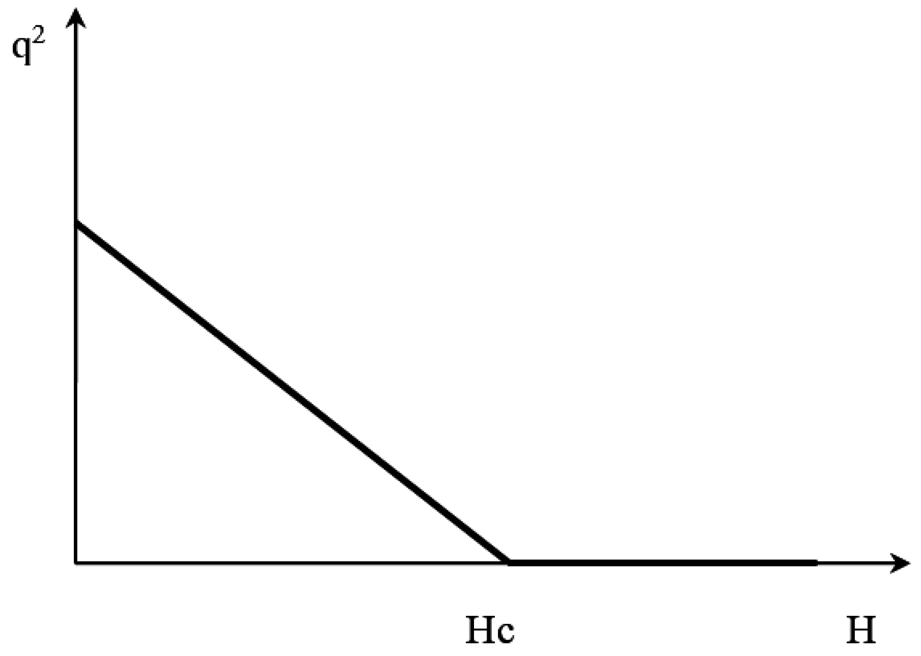
Figure 2 shows a graphical solution of (5), shaped as a phase transition hockey stick. Thus, if the relationship between the order parameter (i.e., the relative abundance of the tree species) and the height of the habitat is described by model (5), we can conclude that the processes leading to the formation of altitudinal vegetation belts can be modeled by using an ecological analog of the model of the second-order phase transitions.

3. Results

Height-dependent changes in the species composition of forest communities can be described by the model of ecological second-order phase transitions. According to this model, there must be a critical height, Hr, from which upwards, the squared relative frequency of occurrence of a particular species, q2(H), and the height, H, of its habitat will be linearly related. Analysis of the forest inventory data for the Sayan Mountains (the south of Middle Siberia) showed that the inventory data on the distribution of different tree species along the height transects were in good agreement with the model proposed in this study. By using the model of second-order phase transitions, we calculated the critical heights for different altitudinal belts of vegetation, determined the boundaries and lengths of the ecotones between different vegetation belts, and found the differences in the critical heights of the ecotones between the south- and north-facing transects.
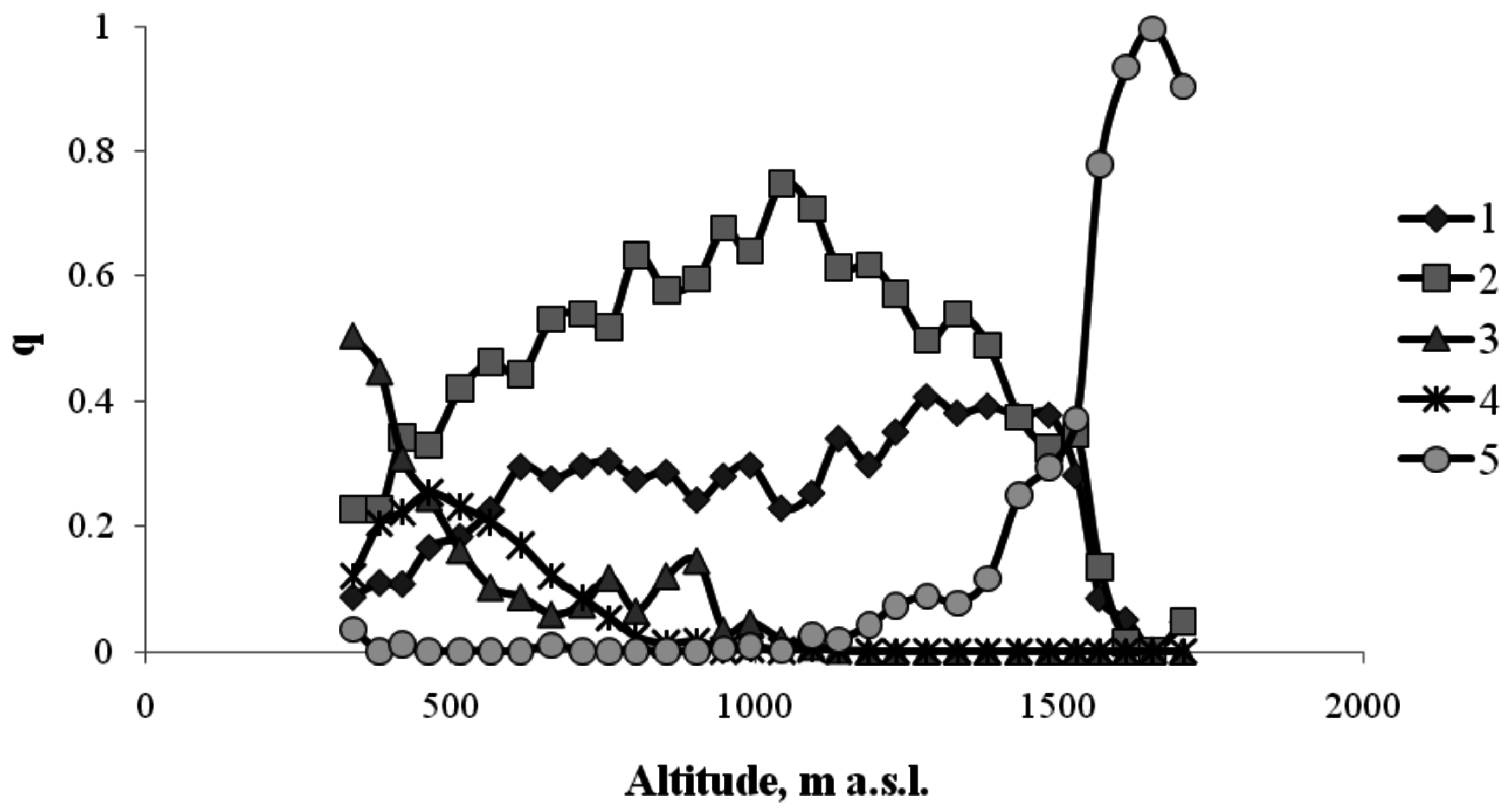
In the altitudinal forest belts of the Sayan Mountains, trees occupy up to 90%–95% of the area. Within the mountain meadow, where there are few or no trees, this percentage is close to zero. Figure 3 shows the frequencies of occurrence of different tree species and species of the meadow community.
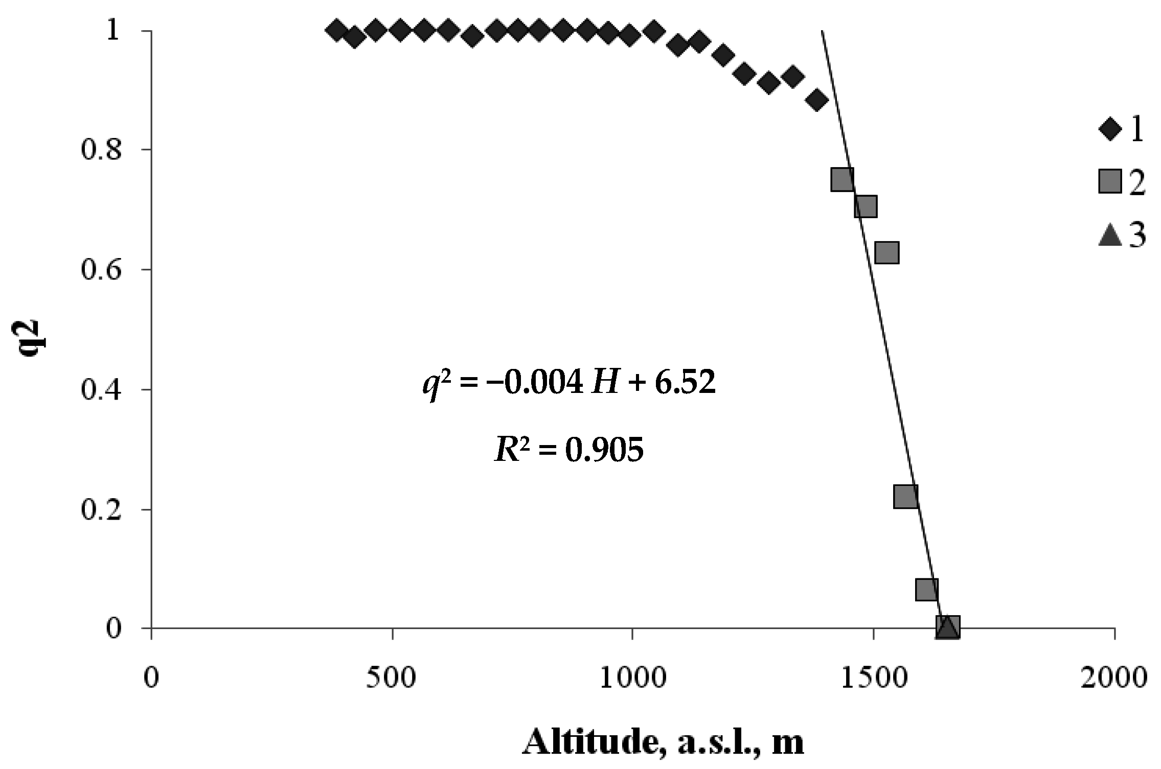
Let us first examine the transition between the mountain forest and the mountain meadow. Here, the order parameter q (0 ≤ q ≤ 1) will be defined as the fraction of the area occupied by forest vegetation at height H. Figure 4 shows the relationship between the value of q2— the squared order parameter and the value of H for the zone of transition between forest vegetation and meadow vegetation.
As shown in Figure 4, below ~1500 m a.s.l., the transect area is almost completely occupied by woody plants (i.e., q ≈ 1 and, hence, q2 ≈ 1). From the critical height, ~1500 m a.s.l., upwards, the squared area occupied by plants monotonically decreases, and at a height of about 1700 m a.s.l., there are almost no woody plants, and this is the boundary of the mountain meadow. The form of the regression equation describing the relationship between q2 and H is similar to the form of theoretical Equation (5). The critical height, Нс, at which the forest is completely replaced by the meadow, is found through the relationship between the regression equation coefficients: H c = 6.52 0.004 = 1629 m. The height, Нm, at which meadow vegetation almost completely vanishes, can be found from the condition, 1 = A B H m i.e., H max = 1380 m. Thus, the vertical extent of the forest–meadow ecotone is about 250 m.
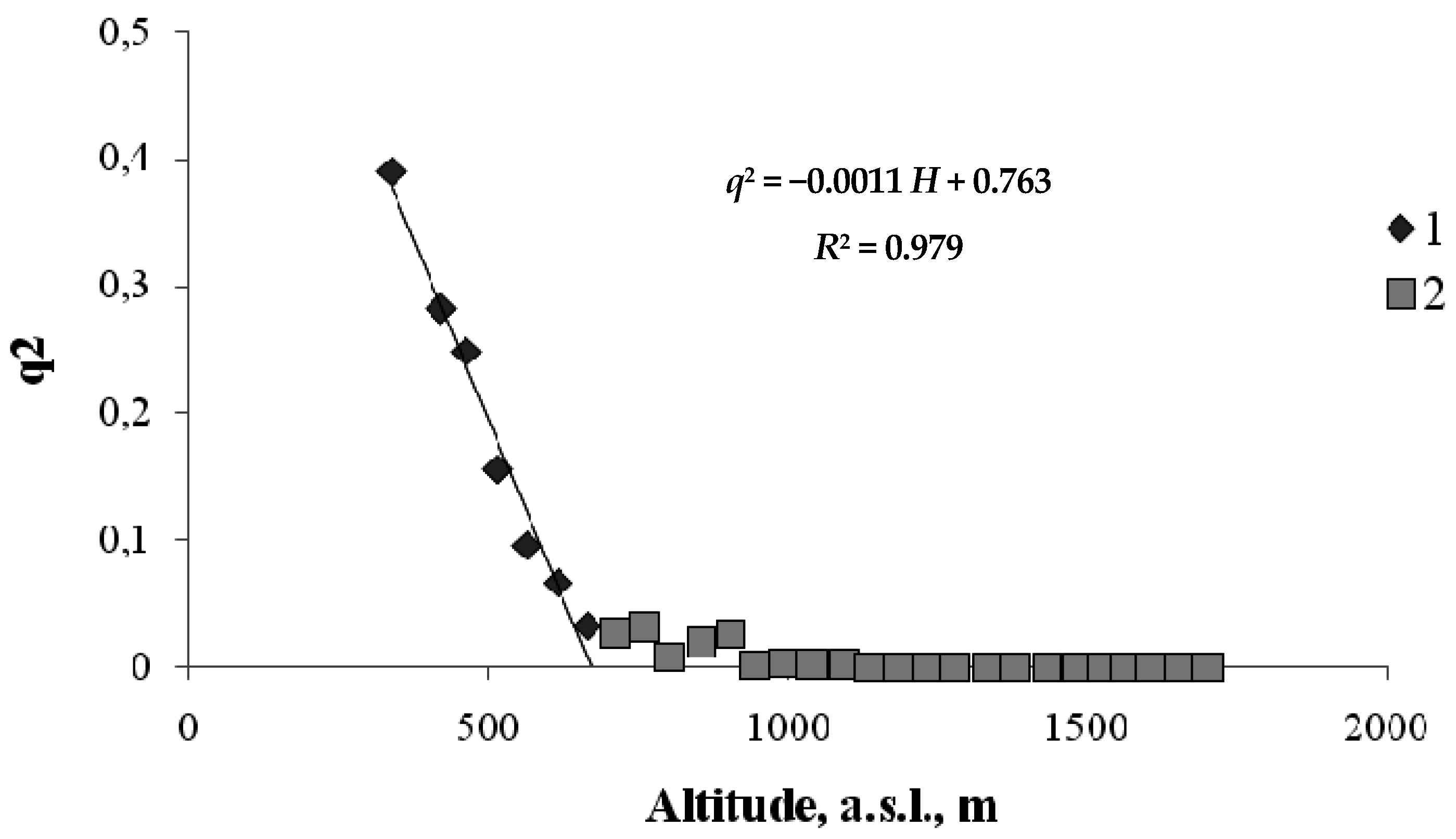
A similar relationship between the squared order parameter and the height of the habitat is found when hardwood tree species (birch and aspen) are replaced by coniferous species (Siberian fir, Siberian pine, and Scots pine) (Figure 5). In this case, the order parameter, q, is the fraction of the area unoccupied by hardwood tree species.
From Figure 5 we can see that hardwood trees occur up to a certain critical height, and, then, conifers completely replace them. From the regression equation for the relationship between q2 and H shown in Figure 5, we can obtain the critical height H d = 0.763 0.0011 = 694   m   a . s . l . at which the coniferous tree belt begins.
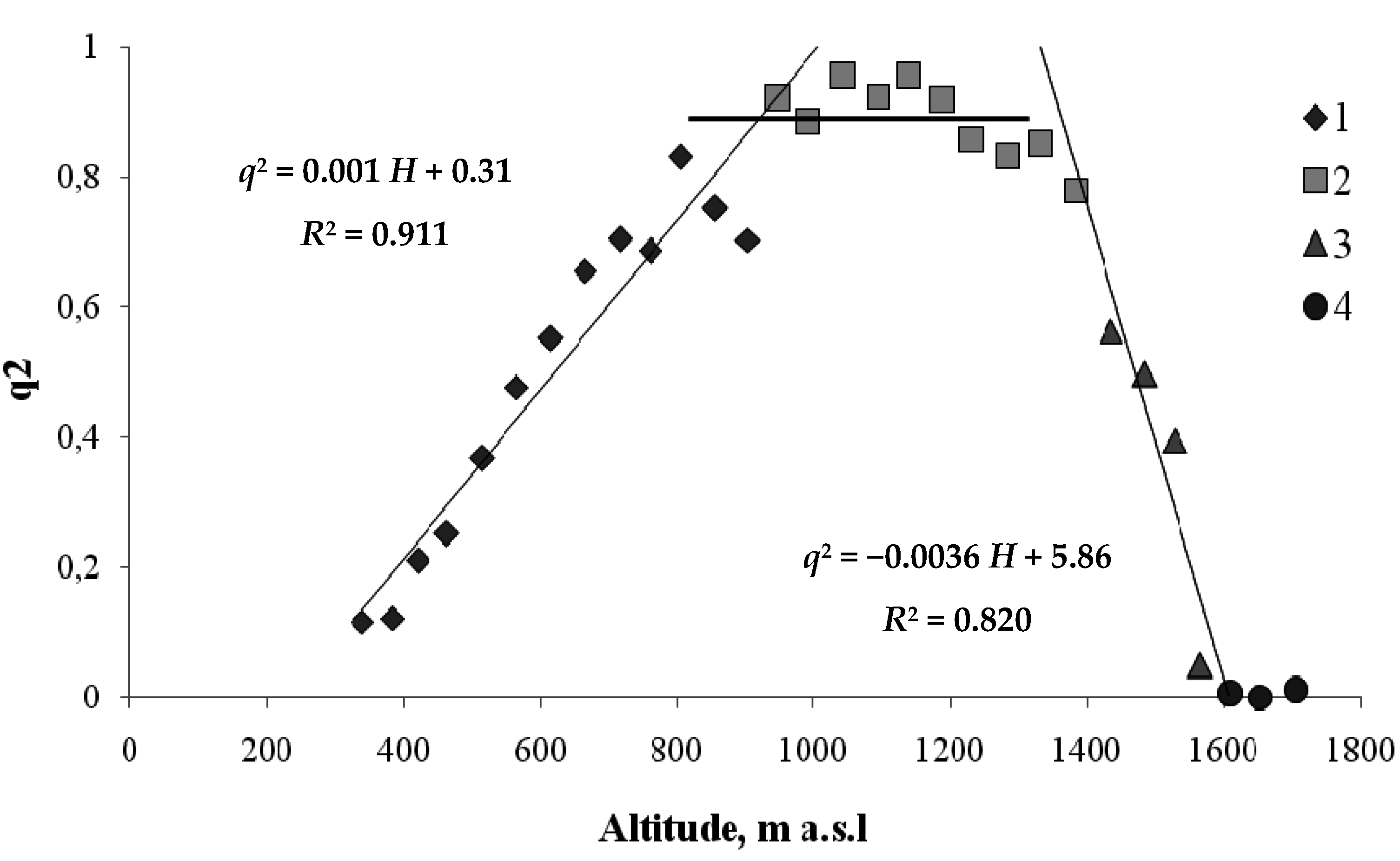
We need a somewhat more complex model to describe the coniferous belt, which in the Sayan Mountains mainly consists of Siberian fir trees. Figure 6 shows the relationship between the squared order parameter q—the fraction of the area occupied by coniferous trees—and the height, H, of the coniferous tree habitat.
As shown in Figure 6, coniferous species, which form a separate belt, prevail at heights between 700 and 1380 m. At heights above 1380, coniferous trees are gradually replaced by meadow vegetation in the ecotone. At heights below 700 m, there is an ecotone in which coniferous trees are gradually replaced by hardwood species.

4. Discussion

Thus, transitions between the altitudinal belt of hardwood trees and the belt of coniferous trees and between the forest belt and the mountain meadow are very well described by the ecological analog of the model of second-order phase transitions. Table 1 characterizes the forest–meadow and hardwood–conifer ecotones for the transects chosen for this study.
As can be seen from Table 1, the upper boundaries of the conifer–mountain meadow ecotones were located at nearly the same heights on the north- and south-facing transects. The lower boundary of the conifer–mountain meadow ecotone of the north-facing transect was, however, 200 m higher than the lower boundary of the corresponding ecotone on the south-facing transect. In addition to that, the vertical extent of the conifer–mountain meadow ecotone was somewhat greater on the south-facing transect.
The transition from the forest belt to the mountain meadow may be caused by the temperature decrease with height and the impairment of the growing conditions for all tree species. Gradual ousting of coniferous trees by hardwood species may characterize interactions between these two groups, additionally modulated by the environmental factors.

4.1. Interactions between Various Tree Species within the Same Altitudinal Belt

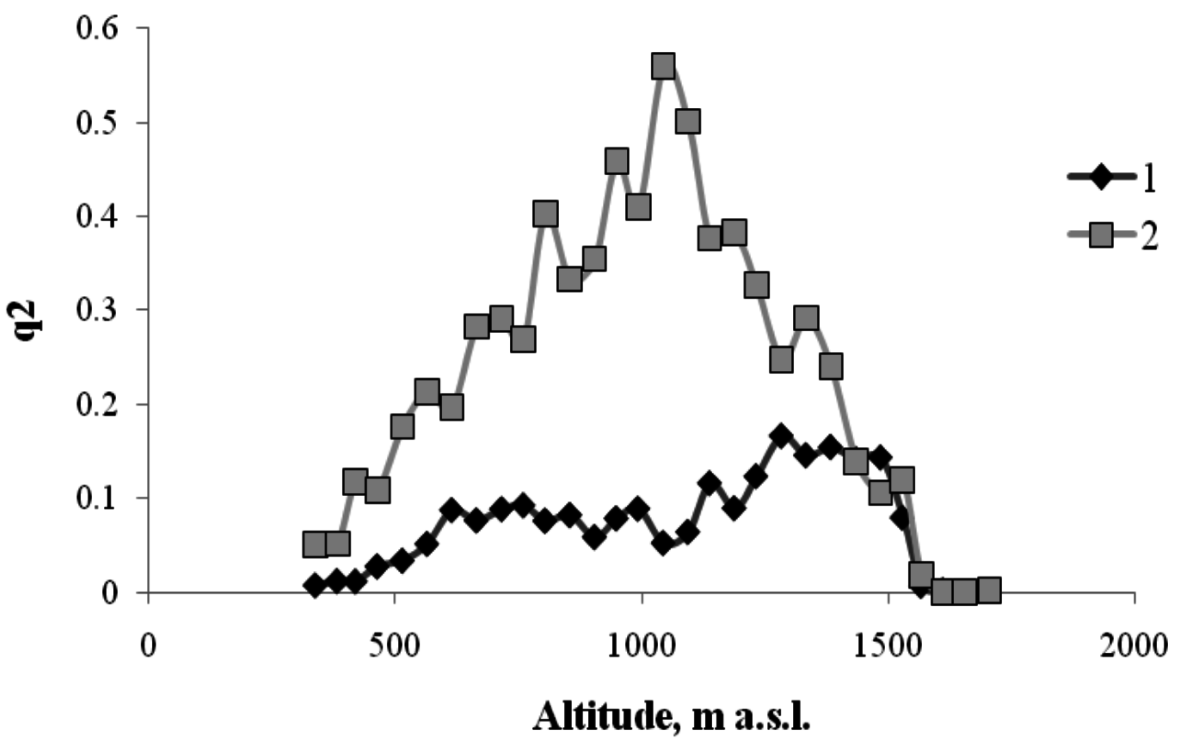
To evaluate interactions between different tree species on the transect, let us examine the coherence of the relationships between the squared order parameter and the inverse height of the habitat of the Siberian fir and Siberian pine (the Siberian pine is a minor species in this community, occupying about 10% of the total area of the transect) (Figure 7).
As shown in Figure 7, within the conifer–mountain meadow ecotone, the values of the order parameters for the fir and the pine decrease synchronously. However, at heights below 1100 m a.s.l., where the order parameter for the fir begins to decline monotonically, the values of the order parameter for the pine remain stable down to about 800 m a.s.l. This may be explained by either the absence of the temperature dependence of the Siberian pine frequency of occurrence or the cooperative effect of Siberian pine–hardwood interactions. The latter seems a more probable reason. Then, by analyzing the coherence of the models of second-order phase transitions for different tree species, we may obtain more data on interactions between different tree species.
Comparison of the properties of the conifer–hardwood ecotones on the north- and south-facing transects confirms temperature dependence of the altitudinal zonation. On the south-facing transect, the conifer–hardwood ecotone is situated between 400 and 600 m a.s.l., while on the north-facing transect, it is situated between 300 and 700 m a.s.l.

4.2. Climate Factors in the Model

Climate is one of the major factors influencing the growth of woody plants. A number of studies have addressed the relationship between temperature and growth of woody plants in the context of global climate change [41,42,43,44,45]. However, models analyzing the relationship between climate factors and tree phytomass increase usually use empirical susceptibility functions, which characterize the effect of temperature on woody plant productivity [46], or accept rather arbitrary rules of the shift of boundaries between ecosystems [47]. The occurrence of the species, though, is influenced not only by climate factors but also by interspecific competition and soil properties. Therefore, it is not correct to describe the spatial structure of woody plants by using only the functions of response to climate factors [48]. In contrast to those models, the proposed theoretical model describes the relationship between survival of the trees of a definite species and ambient temperature. The model can be used to determine the altitudinal threshold (actually related to ambient temperature T) at which trees of the definite species can still grow and estimate the width of the ecotone.
A number of different approaches can be used to describe the influence of climate factors on the position and extent of ecotones using the model of second-order phase transitions. One approach is to renormalize the relationship between temperature T and height H. Under current conditions, this relationship is described by equation T = T0 + kH, but under climate change (e.g., warming), this relationship will be expressed by equation T = T0 + kH + Tadd. Then, according to the model (7), the boundaries of all ecotones will be shifted upwards, i.e., both the upper and the lower boundaries of the conifer–mountain meadow ecotone must be located higher on the south-facing transect. This conclusion, however, is not consistent with the data in Table 1, showing that the upper boundaries of the conifer–mountain meadow ecotone are located at similar heights on the north- and south-facing transects, while the lower boundary of this ecotone is almost 200 m higher on the north-facing transect.
Another approach to describing the influence of climate changes on the position and extent of the ecotone on the mountains is to treat rather small temperature shifts as an additional “field”, h, influencing the particular plant community. Then, Equation (3) can be written as follows:
G ( q ) = G 0 + a ( H H c ) q 2 + b q 4 q h
The stable state of the plant community for model (6) will be also characterized by the minimum of function G(q):
G q = 2 a ( H H c ) q + 4 b q 3 h = 0
If additive term h, describing external field, is introduced into Equation (6) for the potential function, there is no solution q = 0 in Equation (7). However, at low values of h and small differences between height H and critical height Hc, approximate solutions can be used. Then, phase transitions can be still regarded as second-order phase transitions. It would be very interesting to estimate the likelihood of the shift of the conifer–mountain meadow boundary under climate warming. If an additional temperature field, h, is small, in the region where H > Hc and q → 0 (i.e., above the upper boundary of the conifer–mountain meadow ecotone), in model (7), ignoring term q3, we obtain q h 2 a ( H c H ) > 0 . In this case, we should expect the upper boundary of the conifer–meadow ecotone to shift upwards. The higher the value of h and the lower the value of coefficient a, the more the boundary of the conifer–mountain meadow ecotone will rise.
In the region where H < Hc, we can roughly write:
q ( a 2 b ( H c H ) ) 1 / 2 + h 4 a ( H c H )
The first term in (8) is the value of the order parameter if there is no additional field. The second term in (8) depends on the value of the additional field, coefficient a, and the difference ( H c H ) . The greater the values of a and ( H c H ) , the less the order parameter will be different from its value in the absence of the additional field. Thus, for the conifer–meadow phase transition, according to model (8), the lower boundary of the ecotone should not be expected to shift upwards over a considerable distance due to the influence of the additional field.
To describe the effect of temperature changes on the order parameter, which reflects the frequency of occurrence of the particular tree species, one can introduce the susceptibility function, x = q h . The greater the value of the susceptibility function, the greater the change in the plant species composition under temperature change. If, however, x 0 temperature does not influence the plant species composition. The susceptibility function can be written by differentiating (8):
χ = q h = 1 4 a ( H H c )
If | H H c | , then q h 0 , and the effect of the additional temperature field on vegetation will be insignificant.
Thus, an increase in the temperature under possible climate change will primarily influence the position of the upper boundary of the conifer–mountain meadow ecotone and may cause the ecotone to expand.

5. Conclusions

The study shows that the model of ecological second-order phase transitions accurately describes height-dependent changes in the species composition of forest ecosystems. Analysis of forest inventory data for the Sayan Mountains (south Middle Siberia) proved that inventory data on the distribution of different tree species along altitudinal transects are in good agreement with the proposed model. The model of second-order phase transitions can be used to estimate critical heights for different altitudinal belts of vegetation, determine the boundaries and extents of ecotones between different vegetation belts, and reveal differences in the critical heights between ecotones at south- and north-facing transects.
A supplementary model was proposed to describe the shifts of ecotone boundaries due to climate change. The approach proposed in this study can be used to determine the boundaries between plant communities, to estimate the sizes of ecotones between the neighboring communities, and to analyze the shifts in the positions of the communities.
Models of second-order phase transitions are universal models, and, thus, they are successfully used to describe processes that differ considerably from phase transitions in physical systems.
As previously mentioned, the model of second-order phase transitions is static and, unfortunately, cannot describe the dynamics of the ecotone boundary shift. Since the characteristic lifespan of woody plants is several decades or a few hundred years, while the lifespan of herbs is a few years, the upward shift of the forest–meadow on the mountains may be rather quick while the shift of the hardwood–conifer ecotone may take a much longer time. Interactions between different tree species seem to play a significant part in the establishment of the boundaries and the extent of the hardwood–conifer ecotone.

Acknowledgments

The study was supported by RFBR and Krasnoyarsk Regional Science Foundation grant No. 15-45-04034 r_sibir_a.

Author Contributions

V. Soukhovolsky is responsible for the idea to use the second-order phase transition model to describe height-dependent changes in the species composition of mountain forest ecosystems; Y. Ivanova analyzed the data and wrote the main part of the paper.

Conflicts of Interest

The authors declare no conflict of interest.

References

  1. Odum, E.P. Fundamentals of Ecology; W.B. Saunders Company: Philadelphia, PA, USA, 1953; p. 384. [Google Scholar]
  2. Whittaker, R.H. Communities and Ecosystems; Macmillan Publishing Co., Inc.: New York, NY, USA, 1975; p. 158. [Google Scholar]
  3. Auer, S.K.; King, D.I. Ecological and life-history traits explain recent boundary shifts in elevation and latitude of western North American songbirds. Glob. Ecol. Biogeogr. 2014, 23, 867–875. [Google Scholar] [CrossRef]
  4. Chen, I.-C.; Hill, J.K.; Ohlemuller, R.; Roy, D.B.; Thomas, C.D. Rapid range shifts of species associated with high levels of climate warming. Science 2011, 333, 1024–1026. [Google Scholar] [CrossRef] [PubMed]
  5. Pacifici, M.; Foden, W.B.; Visconti, P.; Watson, J.E.M.; Butchart, S.H.M.; Kovacs, K.M.; Scheffers, B.R.; Hole, D.G.; Martin, T.G.; Akcakaya, H.R.; et al. Assessing species vulnerability to climate change. Nat. Clim. Chang. 2015, 5, 215–224. [Google Scholar] [CrossRef] [Green Version]
  6. Parmesan, C.; Yohe, G. A globally coherent fingerprint of climate change impacts across natural systems. Nature 2003, 421, 37–42. [Google Scholar] [CrossRef] [PubMed]
  7. Feagan, R. The place of food: Mapping out the ‘local’ in local food systems. Prog. Hum. Geogr. 2007, 31, 23–42. [Google Scholar] [CrossRef]
  8. Kelly, A.E.; Goulden, M.L. Rapid shifts in plant distribution with recent climate change. Proc. Natl. Acad. Sci. USA 2008, 105, 11823–11826. [Google Scholar] [CrossRef] [PubMed]
  9. Lenoir, J.; Gugout, J.C.; Marquet, P.A.; de Ruffray, P.; Brisse, H. A significant upward shift in plant species optimum elevation during the 20th century. Science 2008, 320, 1768–1771. [Google Scholar] [CrossRef] [PubMed]
  10. Moritz, C.; Agudo, R. The future of species under climate change: Resilience or decline? Science 2013, 341, 504–508. [Google Scholar] [CrossRef] [PubMed]
  11. Parmesan, C. Ecological and evolutionary responses to recent climate change. Annu. Rev. Ecol. Evol. Syst. 2006, 37, 637–669. [Google Scholar] [CrossRef]
  12. Root, T.L.; Price, J.T.; Hall, K.R.; Schneider, S.H.; Rosenzweig, C.; Pounds, J.A. Fingerprints of global warming on wild animals and plants. Nature 2003, 421, 57–60. [Google Scholar] [CrossRef] [PubMed]
  13. Walther, G.-R.; Beizner, S.; Burga, C.A. Trends in the upward shift of alpine plants. J. Veg. Sci. 2005, 16, 541–548. [Google Scholar] [CrossRef]
  14. Grabherr, G.; Gottfried, M.; Pauli, H. Climate effects on mountain plants. Nature 1994, 369, 448. [Google Scholar] [CrossRef] [PubMed]
  15. Loarie, S.R.; Duffy, P.B.; Hamilton, H.; Asner, G.P.; Field, C.B.; Ackerly, D.D. The velocity of climate change. Nature 2009, 462, 1052–1055. [Google Scholar] [CrossRef] [PubMed]
  16. Ordonez, A.; Williams, J.W. Climatic and biotic velocities for woody taxa distributions over the last 16,000 years in eastern North America. Ecol. Lett. 2013, 16, 773–781. [Google Scholar] [CrossRef] [PubMed]
  17. Kosanic, A.; Anderson, K.; Frure, C.H.; Harrison, S. Regional vegetation change and implications for local conservation: An example from West Cornwall (United Kingdom). Glob. Ecol. Concerv. 2015, 4, 405–413. [Google Scholar] [CrossRef]
  18. Prach, K.; Rauch, O. On filter effects of ecotones. Ecologia (CSFR) 1992, 11, 293–298. [Google Scholar]
  19. Janik, J. Ecotone and ecocline: Two questenable concepts in ecology. Ecologia (CSFR) 1992, 11, 243–250. [Google Scholar]
  20. Hickey, M.B.C.; Doran, B. A review of the efficiency of buffer strips for the maintenance and enhancement of riparian ecosystems. Water Qual. Res. J. Can. 2004, 39, 311–317. [Google Scholar]
  21. Chen, X.-W. Modeling the effects of global climate change at the ecotone of boreal larch forest and temperate forest in Northeast China. Clim. Chang. 2002, 55, 77–97. [Google Scholar] [CrossRef]
  22. Peters, D.P.C.; Gosz, J.R.; Pockman, W.T.; Small, E.E.; Parmenter, R.R.; Collins, S.L.; Muldavin, E. Integrating patch and boundary dynamics to understand and predict biotic transitions at multiple scales. Landsc. Ecol. 2006, 21, 19–33. [Google Scholar] [CrossRef]
  23. Fortin, M.-J. Edge detection algorithms for two-dimensional ecological data. Ecology 1994, 75, 956–965. [Google Scholar] [CrossRef]
  24. Jacquez, G.M.; Maruca, S.; Fortin, M.J. From fields to objects: A review of geographic boundary analysis. J. Geogr. Syst. 2000, 2, 221–241. [Google Scholar] [CrossRef]
  25. Fisher, P.; Arnot, C.; Wadsworth, R.; Wellens, J. Detecting change in vague interpretations of landscapes. Ecol. Inform. 2006, 1, 163–178. [Google Scholar] [CrossRef]
  26. Hufkens, K.; Ceulemans, R.; Scheunders, P. Estimating the ecotone width in patchy ecotones using a sigmoid wave approach. Ecol. Inform. 2008, 3, 97–104. [Google Scholar] [CrossRef]
  27. Hufkens, K.; Scheunders, P.; Ceulemans, R. Ecotones: Methodology and definitions revisited. Ecol. Res. 2009, 24, 977–986. [Google Scholar] [CrossRef]
  28. Hobbs, R.J. Remote sensing of spatial and temporal dynamics of vegetation. In Remote Sensing of Biosphere Functioning; Hobbs, R.J., Mooney, H.A., Eds.; Springer: New York, NY, USA, 1990; pp. 203–219. [Google Scholar]
  29. Csillag, F.; Kabos, S. Wavelets, boundaries, and the spatial analysis of landscape pattern. Ecoscience 2002, 9, 177–190. [Google Scholar] [CrossRef]
  30. Nystrom, M.; Holmgren, J.; Olsson, H. Prediction of tree biomass in the forest–tundra ecotone using airborne laser scanning. Remote Sens. Environ. 2012, 123, 271–279. [Google Scholar] [CrossRef]
  31. Heiskanen, J. Estimating aboveground tree biomass and leaf area index in a mountain birch forest using ASTER satellite data. Int. J. Remote Sens. 2006, 27, 1135–1158. [Google Scholar] [CrossRef]
  32. Hill, R.A.; Granica, K.; Smith, G.M.; Schardt, M. Representation of an alpine treeline ecotone in SPOT 5 HRG data. Remote Sens. Environ. 2007, 110, 458–467. [Google Scholar] [CrossRef]
  33. Ranson, K.J.; Sun, G.; Kharuk, V.I.; Kovacs, K. Assessing tundra-taiga boundary with multi-sensor satellite data. Remote Sens. Environ. 2004, 93, 283–295. [Google Scholar] [CrossRef]
  34. Weiss, D.J.; Walsh, S.J. Remote sensing of mountain environments. Geogr. Compass 2009, 3, 1–21. [Google Scholar] [CrossRef]
  35. Zhang, Y.J.; Xu, M.; Adams, J.; Wang, X.C. Can Landsat imagery detect tree line dynamics? Int. J. Remote Sens. 2009, 30, 1327–1340. [Google Scholar] [CrossRef]
  36. Polikarpov, N.P.; Chebakova, N.M.; Nazimova, D.I. Klimat i Gornyye Lesa Yuzhnoy Sibiri (Climate and Mountain Forests in South Siberia); Novosibirsk: Nauka, Russia, 1986; p. 225. (In Russian) [Google Scholar]
  37. Soukhovolsky, V.G.; Ovchinnikova, T.M.; Baboy, S.D. Altitudinal zonation of tree species in the Sayan Mountains: A model of ecological second-order phase transitions. Zhurnal Obshchey Biologii 2014, 75, 38–47. (In Russian) [Google Scholar]
  38. Landau, L.D.; Lifshitz, E.M. Statistical Physics; Pergamon Press: Oxford, UK, 1980; pp. 501–535. [Google Scholar]
  39. Bruce, A.D.; Cowley, R.A. Structural Phase Transitions; Taylor & Francis: London, UK, 1981; pp. 97–125. [Google Scholar]
  40. Ricklefs, R.E.; Miller, G.L. Ecology; W.H. Freeman & Co.: New York, NY, USA, 2000; p. 822. [Google Scholar]
  41. Matala, J.; Ojansuu, R.; Peltola, H.; Raitio, H.; Kellomaki, S. Modelling the response of tree growth to temperature and CO2 elevation as related to the fertility and current temperature sum of a site. Ecol. Model. 2006, 199, 39–52. [Google Scholar] [CrossRef]
  42. Chmura, D.J.; Anderson, P.D.; Howe, G.T.; Harrington, C.A.; Halofsky, J.E.; Peterson, D.L.; Shaw, D.C.; St. Clair, J.B. Forest responses to climate change in the northwestern United States: Ecophysiological foundations for adaptive management. For. Ecol. Manag. 2011, 261, 1121–1142. [Google Scholar] [CrossRef]
  43. Dale, V.H.; Joyce, L.A.; McNulty, S.; Neilson, R.P.; Ayres, M.P.; Flannigan, M.D.; Hanson, P.J.; Irland, L.C.; Lugo, A.E.; Peterson, C.J.; et al. Climate change and forest disturbances. Bioscience 2001, 51, 723–734. [Google Scholar] [CrossRef]
  44. Briceno-Elizondo, E.; Garcia-Gonzalo, J.; Peltola, H.; Matala, J.; Kellomaki, S. Sensitivity of growth of Scots pine, Norway spruce and silver birch to climate change and forest management in boreal conditions. For. Ecol. Manag. 2006, 232, 152–167. [Google Scholar] [CrossRef]
  45. Bergh, J.; Freeman, M.; Sigurdsson, B.; Kellomäki, S.; Laitinen, K.; Niinistö, S.; Peltola, H.; Linder, S. Modelling the short-term effects of climate change on the productivity of selected tree species in Nordic countries. For. Ecol. Manag. 2003, 183, 327–340. [Google Scholar] [CrossRef]
  46. Condés, S.; García-Robredo, F. An empirical mixed model to quantify climate influence on the growth of Pinus halepensis Mill. stands in South-Eastern Spain. For. Ecol. Manag. 2012, 284, 59–68. [Google Scholar] [CrossRef] [Green Version]
  47. Favier, C.; Chave, J.; Fabing, A.; Schwartz, D.; Dubois, M. Modelling forest–savanna mosaic dynamics in man-influenced environments: Effects of fire, climate and soil heterogeneity. Ecol. Model. 2004, 171, 85–102. [Google Scholar] [CrossRef]
  48. Loehle, C.; LeBlanc, D. Model-based assessments of climate change effects on forests: A critical review. Ecol. Model. 1996, 90, 1–31. [Google Scholar] [CrossRef]
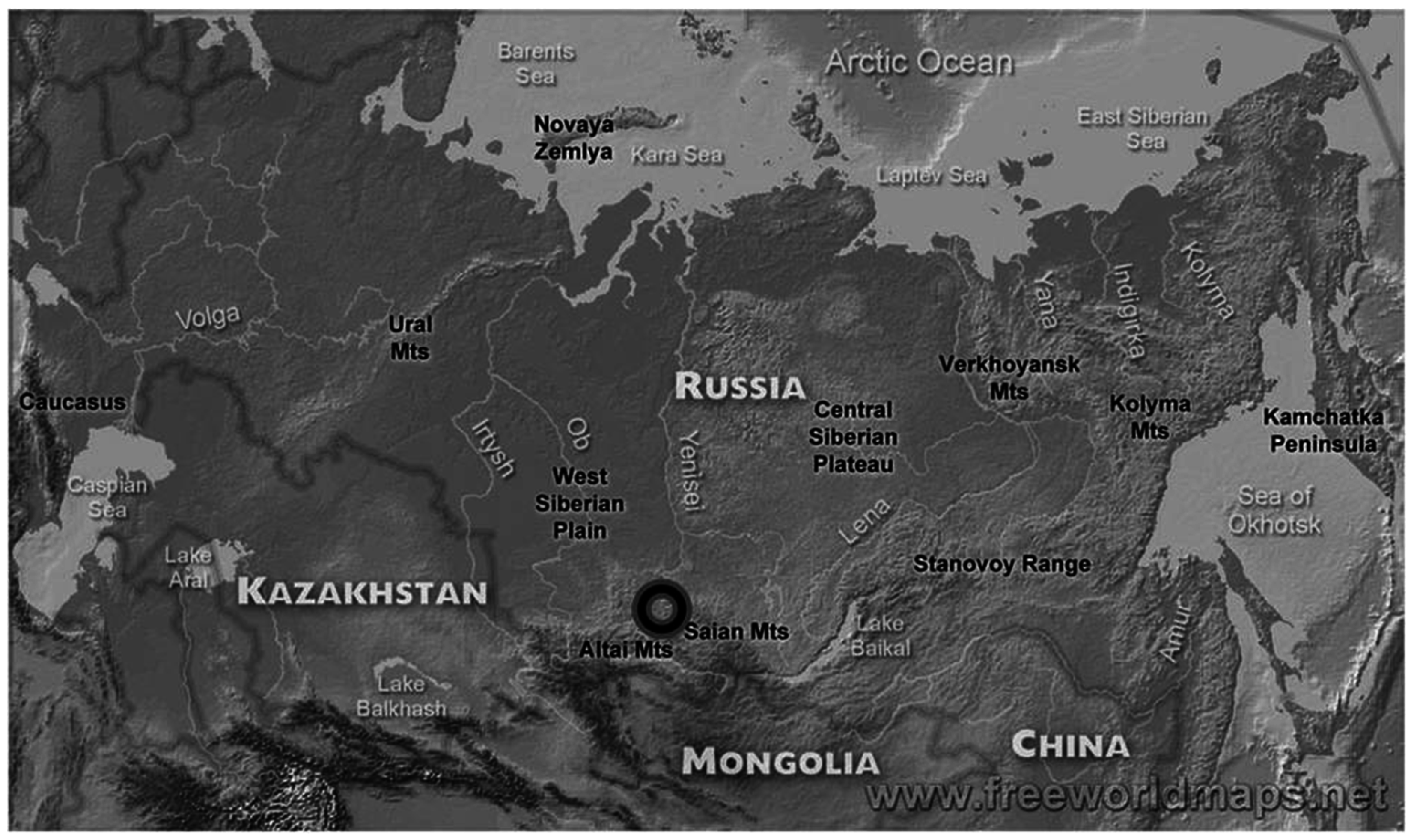
Figure 1. Study site location.
Forests 07 00271 g001
Figure 2. Graphical solution of Equation (5).
Forests 07 00271 g002
Figure 3. The frequency of occurrence of different plant species in the Sayan Mountains along the north-facing transect (1—Siberian pine; 2—Siberian fir; 3—birch; 4—aspen; 5—mountain meadow).
Forests 07 00271 g003
Figure 4. The frequency of occurrence of the trees versus the height of the habitats along the north-facing transect (1—forest belt (hardwood and coniferous); 2—the forest—mountain meadow ecotone; 3—the mountain meadow belt).
Forests 07 00271 g004
Figure 5. Order parameter versus height for the hardwood–conifer ecotone on the north-facing transect (1—ecotone; 2—coniferous belt).
Forests 07 00271 g005
Figure 6. Order parameter versus height for the boundaries of coniferous tree habitats on the north-facing transect (1—hardwood–conifer ecotone; 2—the range of coniferous trees; 3—conifer–mountain meadow ecotone; 4—mountain meadow).
Forests 07 00271 g006
Figure 7. Height-related changes in the values of squared order parameter, q2, for the Siberian fir and Siberian pine (1—Siberian pine; 2—fir; order parameters—fractions of the area at heights H occupied by the trees of these species).
Forests 07 00271 g007
Table 1. Characteristics of the meadow and hardwood conifer ecotones *.
SlopeCritical Heights *Ecotone
Hardwood–ConiferConifer–Meadow
South-facingLB4201157
UB6001610
Н180453
North-facingLB3081380
UB6941627
Н386247
* LB—the lower boundary of the ecotone, m a.s.l.; UB—the upper boundary of the ecotone, m a.s.l.; H—the vertical extent of the ecotone, m.