
Assessment of Aboveground Woody Biomass Dynamics Using Terrestrial Laser Scanner and L-Band ALOS PALSAR Data in South African Savanna

 ,
,
Abstract
:1. Introduction
2. Materials and Methods
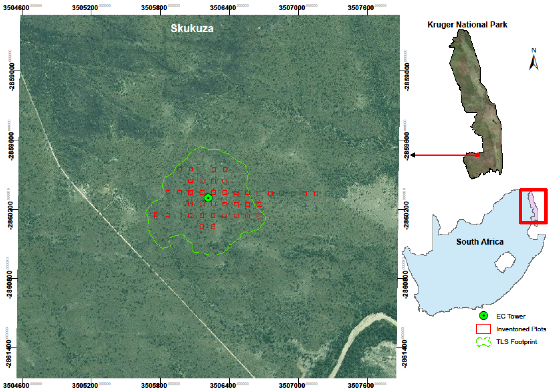
2.1. Study Area
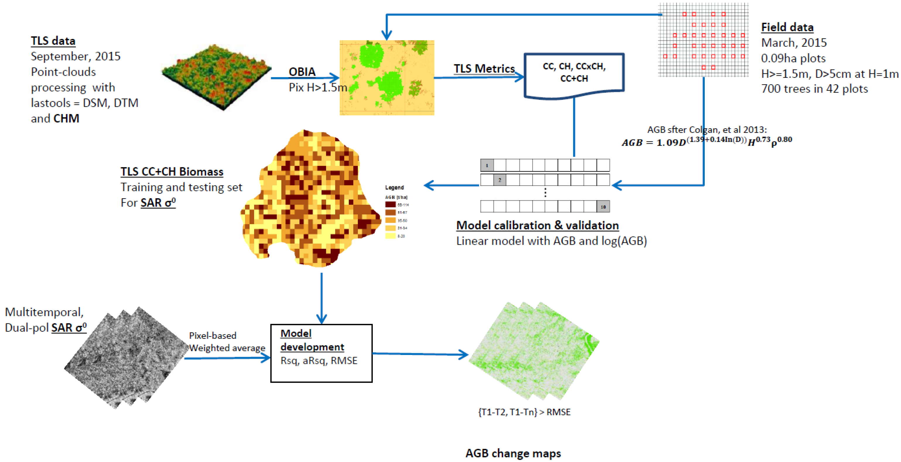
2.2. Summary on Methodology
2.3. Data Acquisition and Processing
2.3.1. Field Inventory Data
2.3.2. Terrestrial Laser Scanner (TLS) Canopy Height Model (CHM)
2.3.3. LOS PALSAR L-Band Data
2.4. Aboveground Biomass (AGB) Modeling
2.4.1. Field Derived Biomass
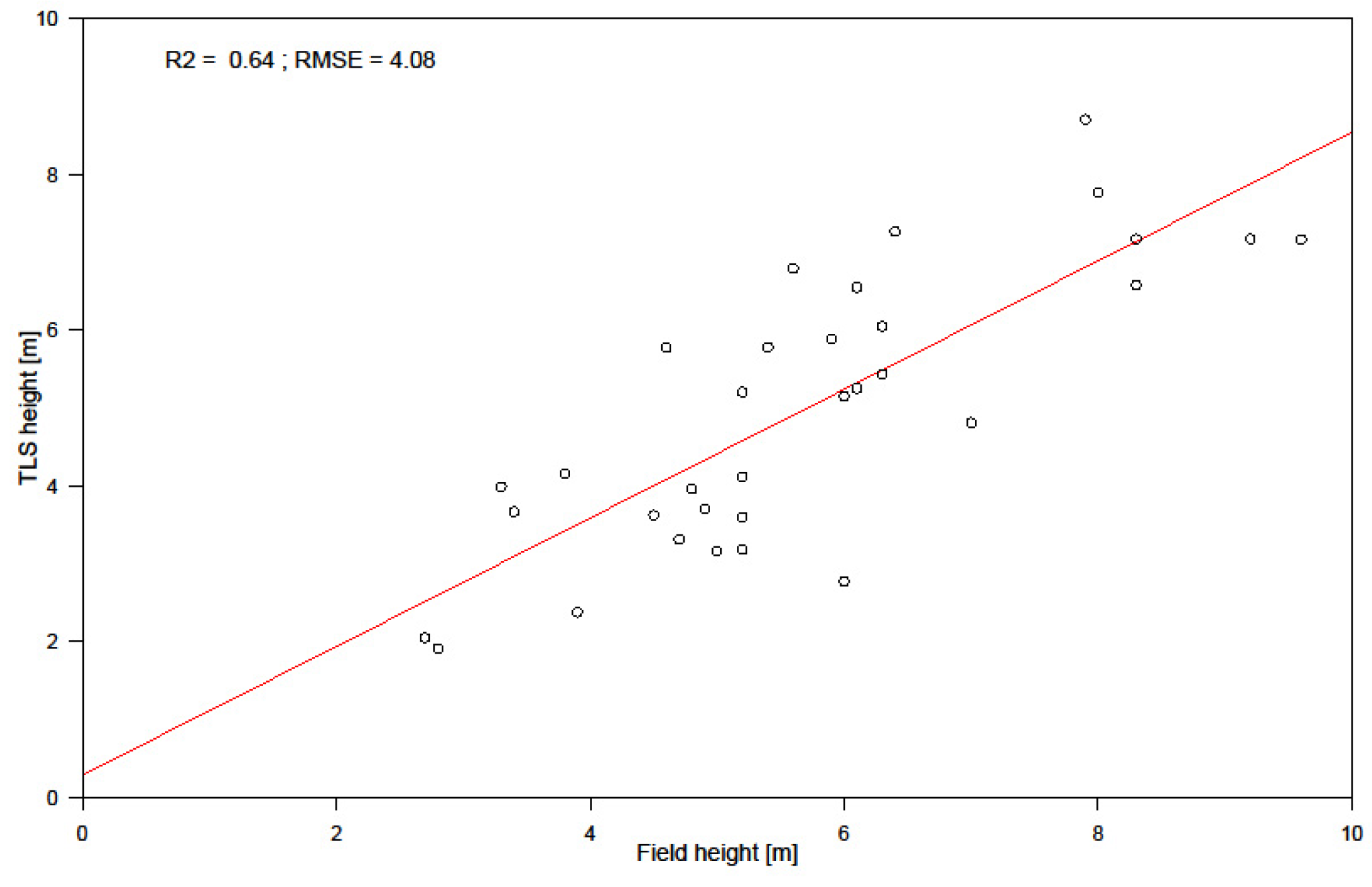
2.4.2. TLS CHM-Derived Biomass
2.4.3. Estimating Aboveground Biomass from SAR
2.4.4. Aboveground Biomass Change Analysis
3. Results
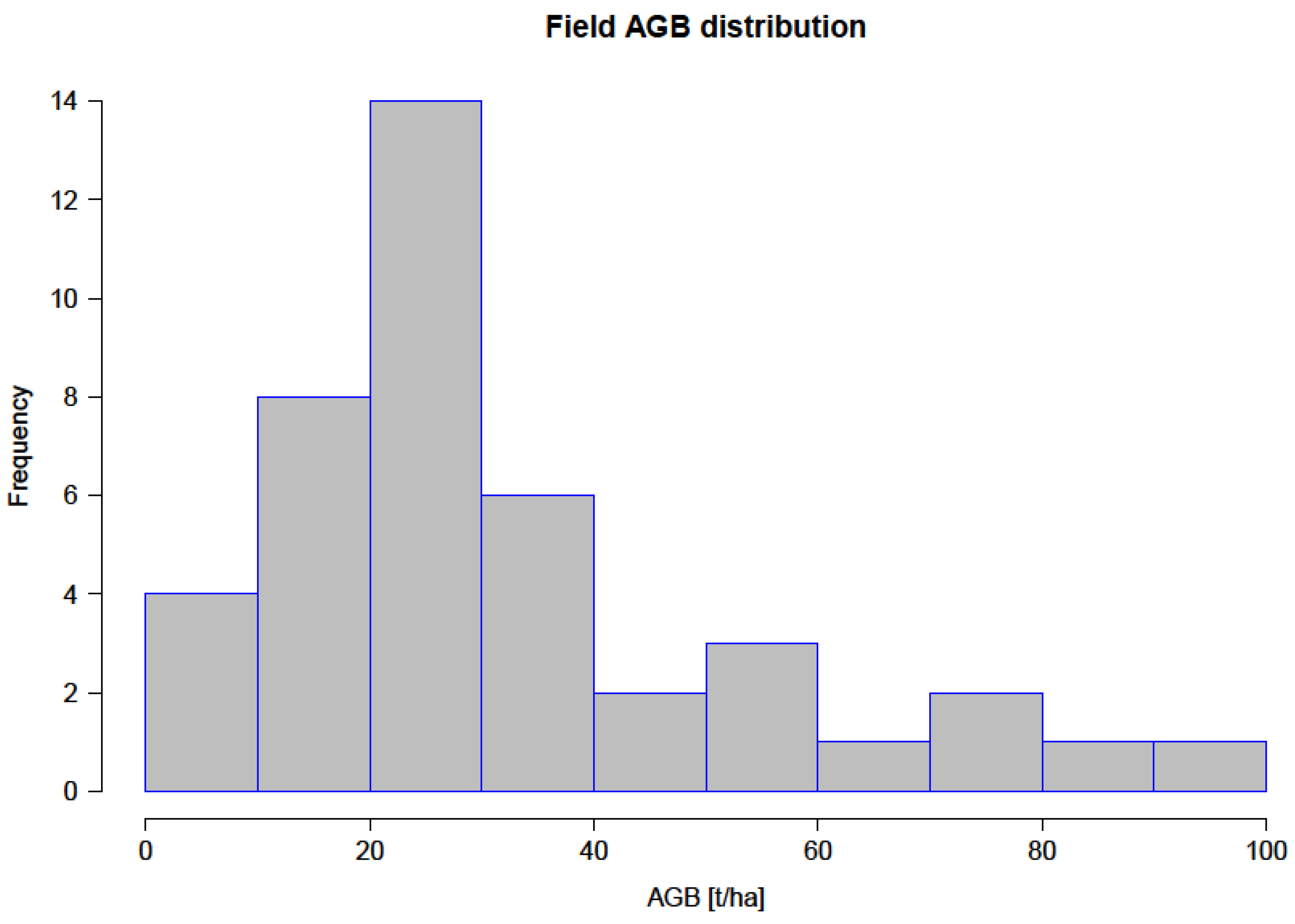
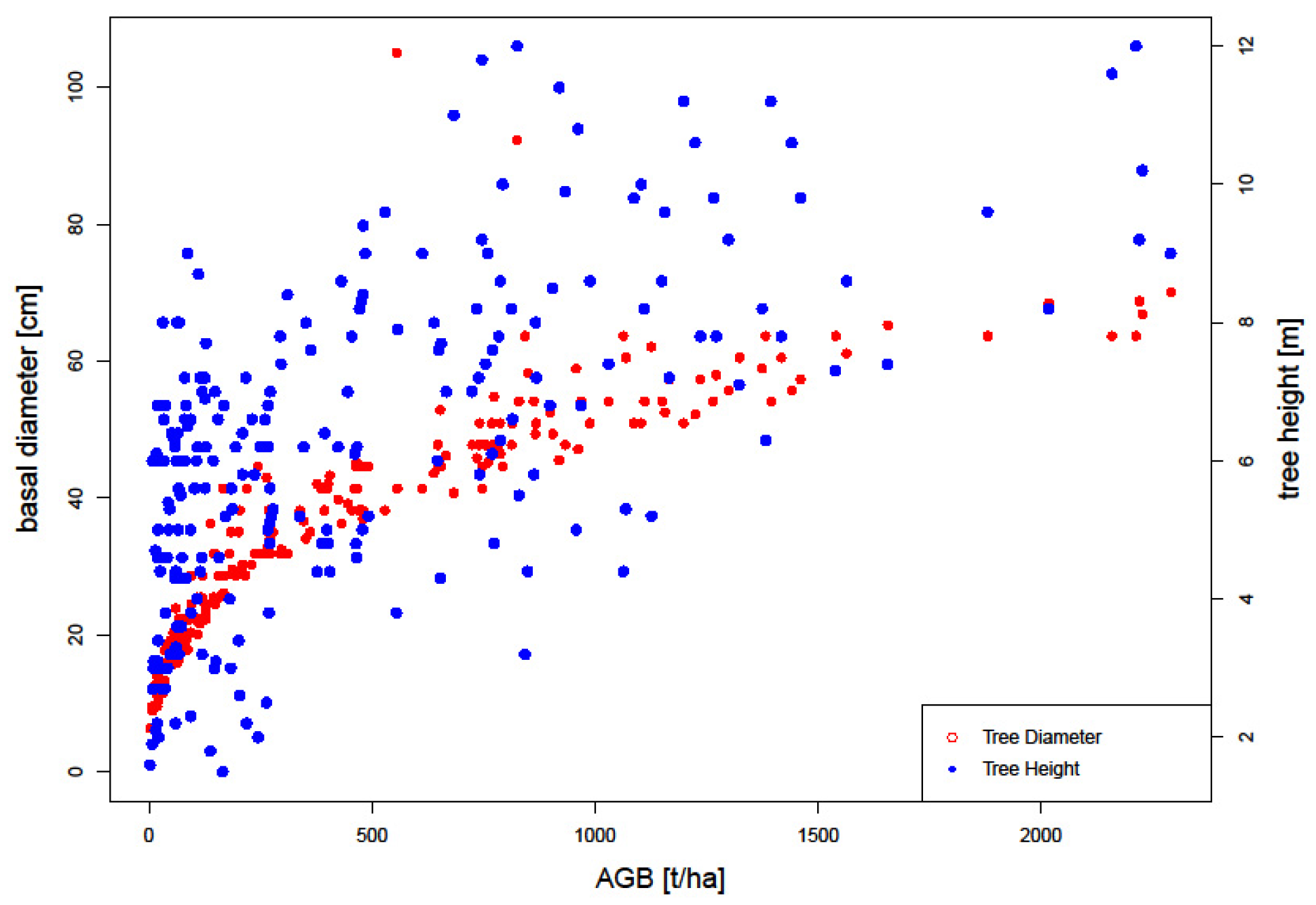
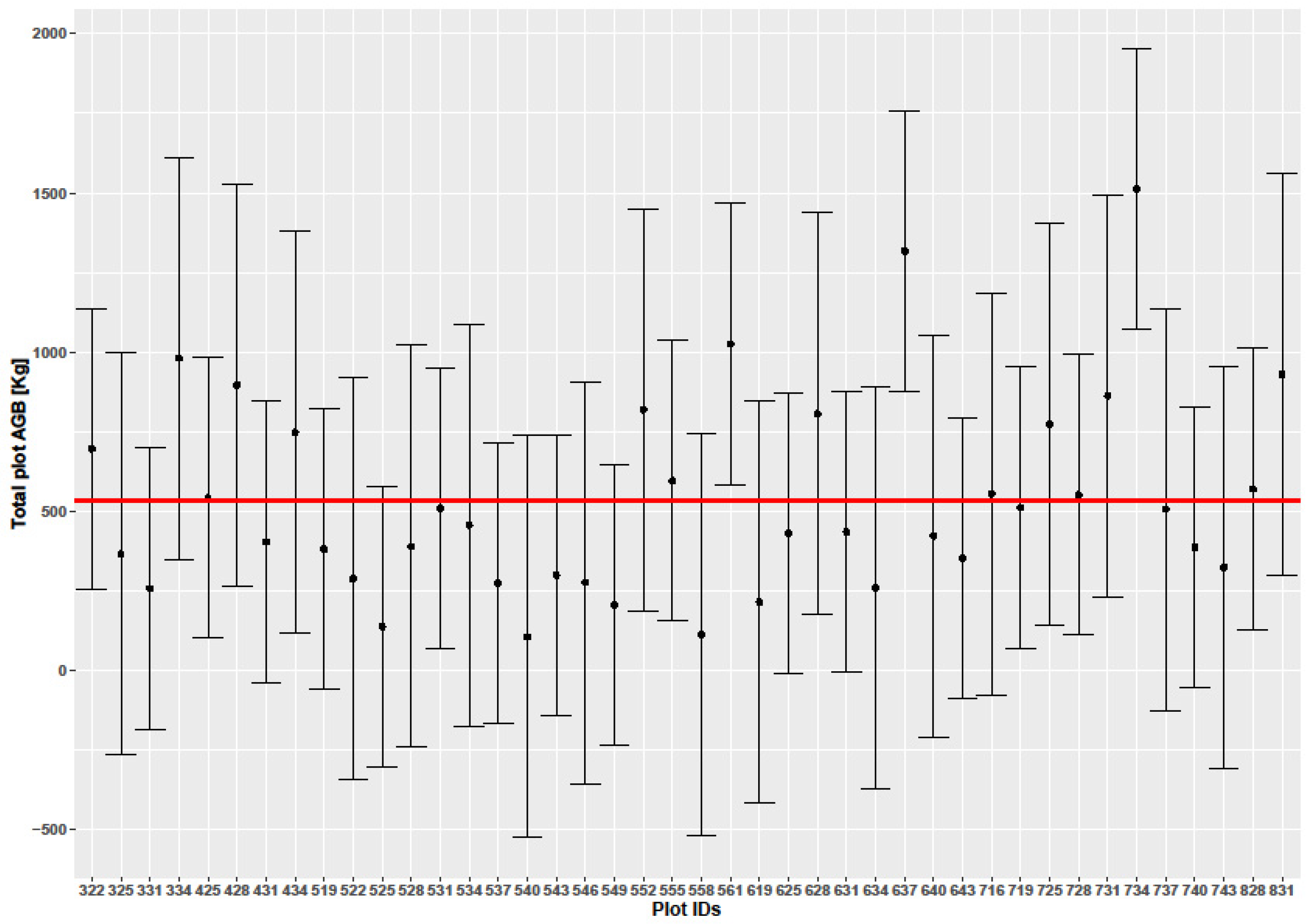
3.1. Field Biomass
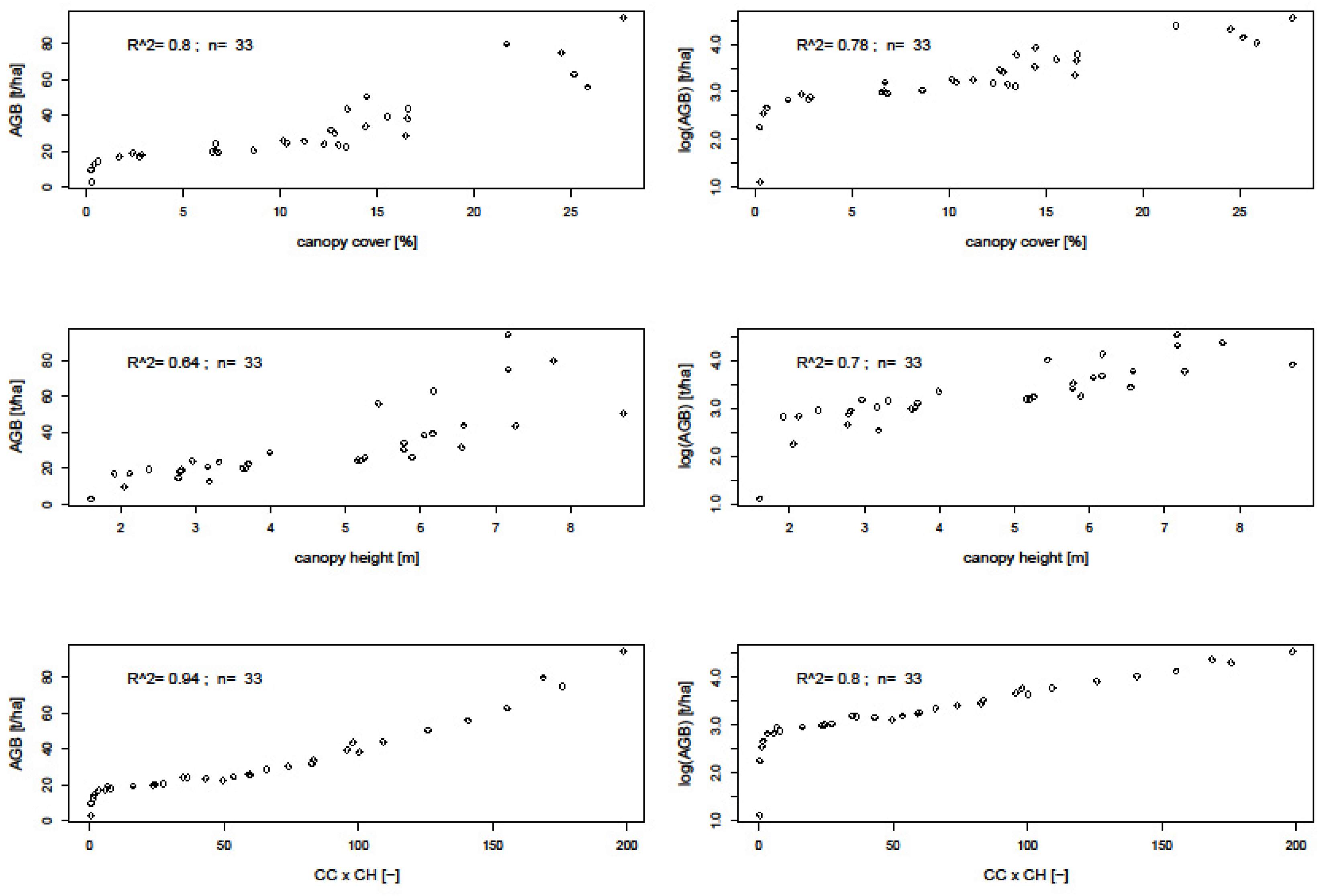
3.2. Biomass Prediction Models
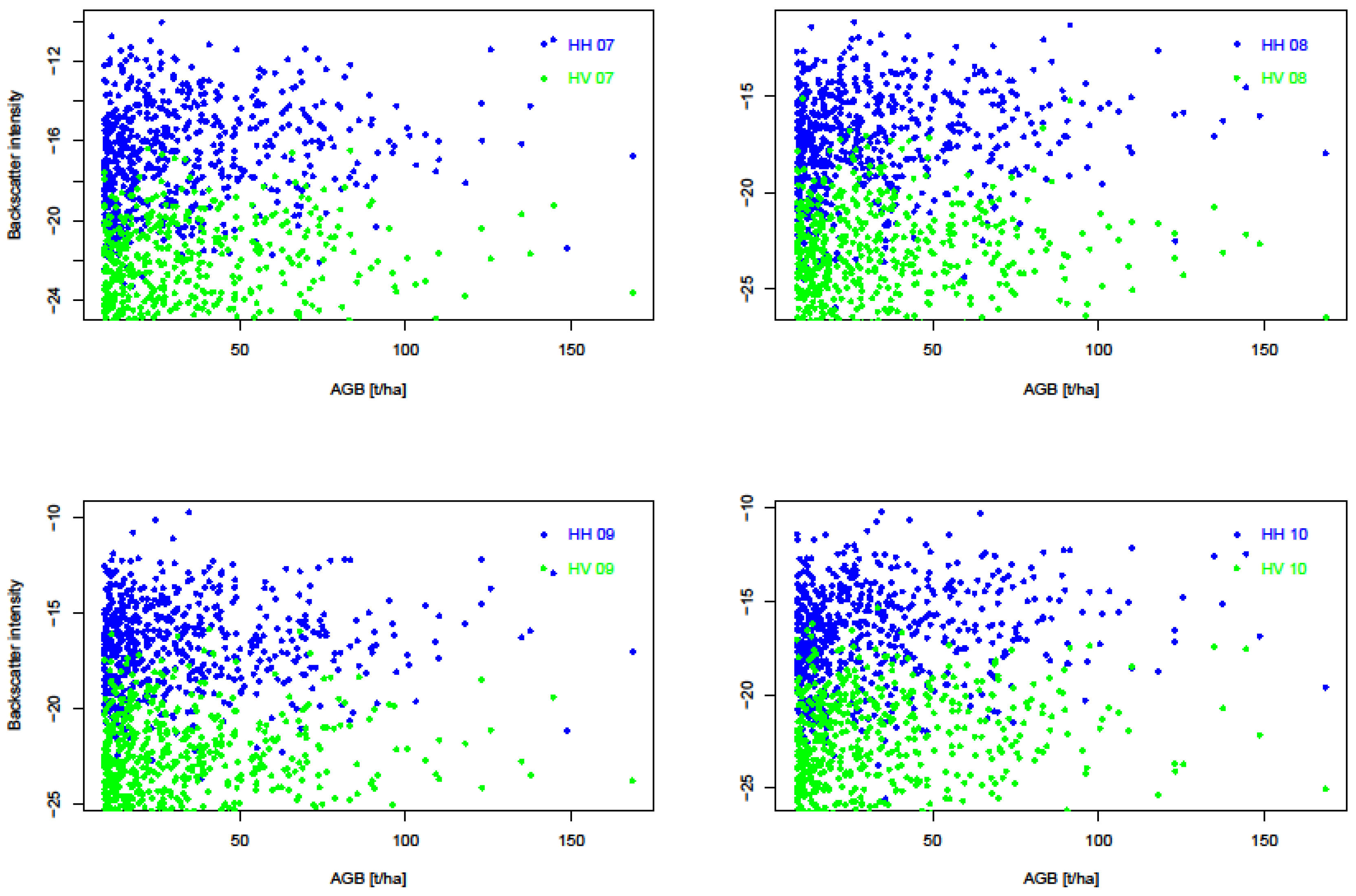
3.3. Radar Sensitivity to Biomass
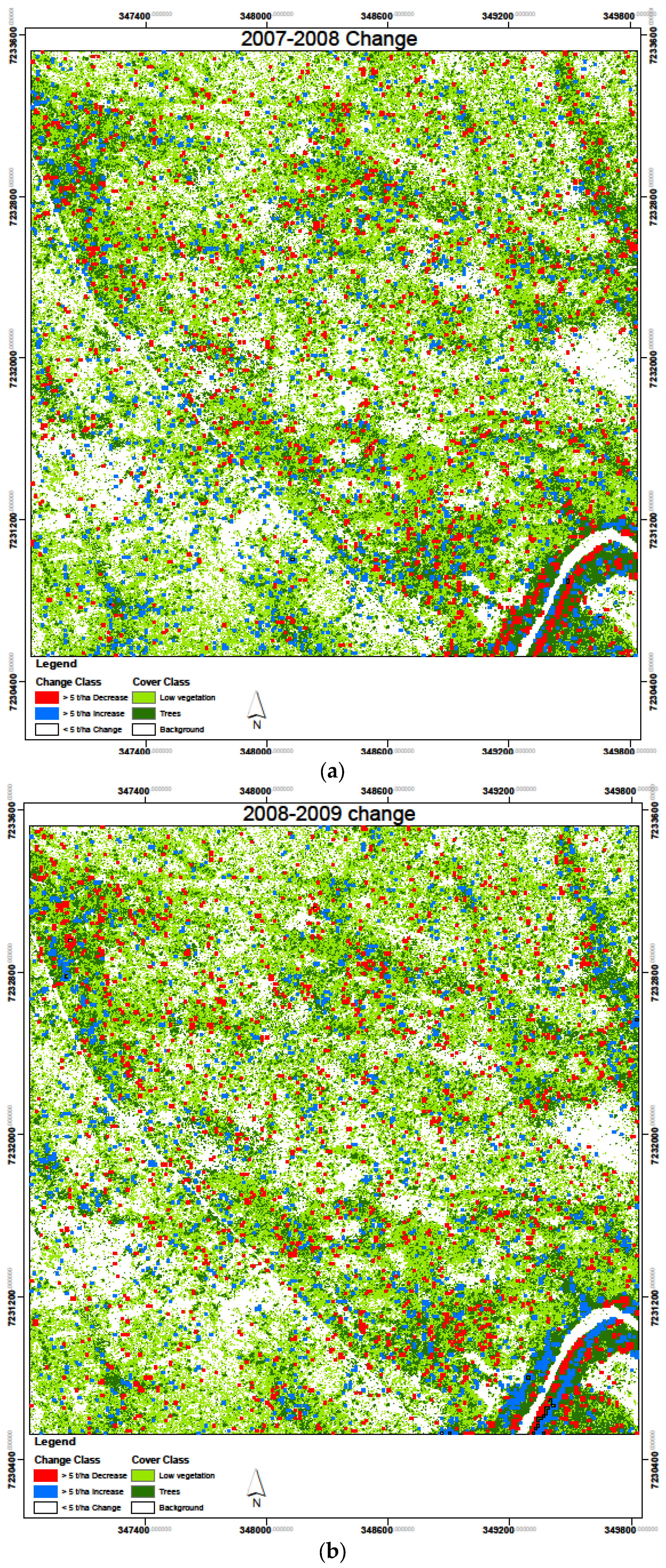
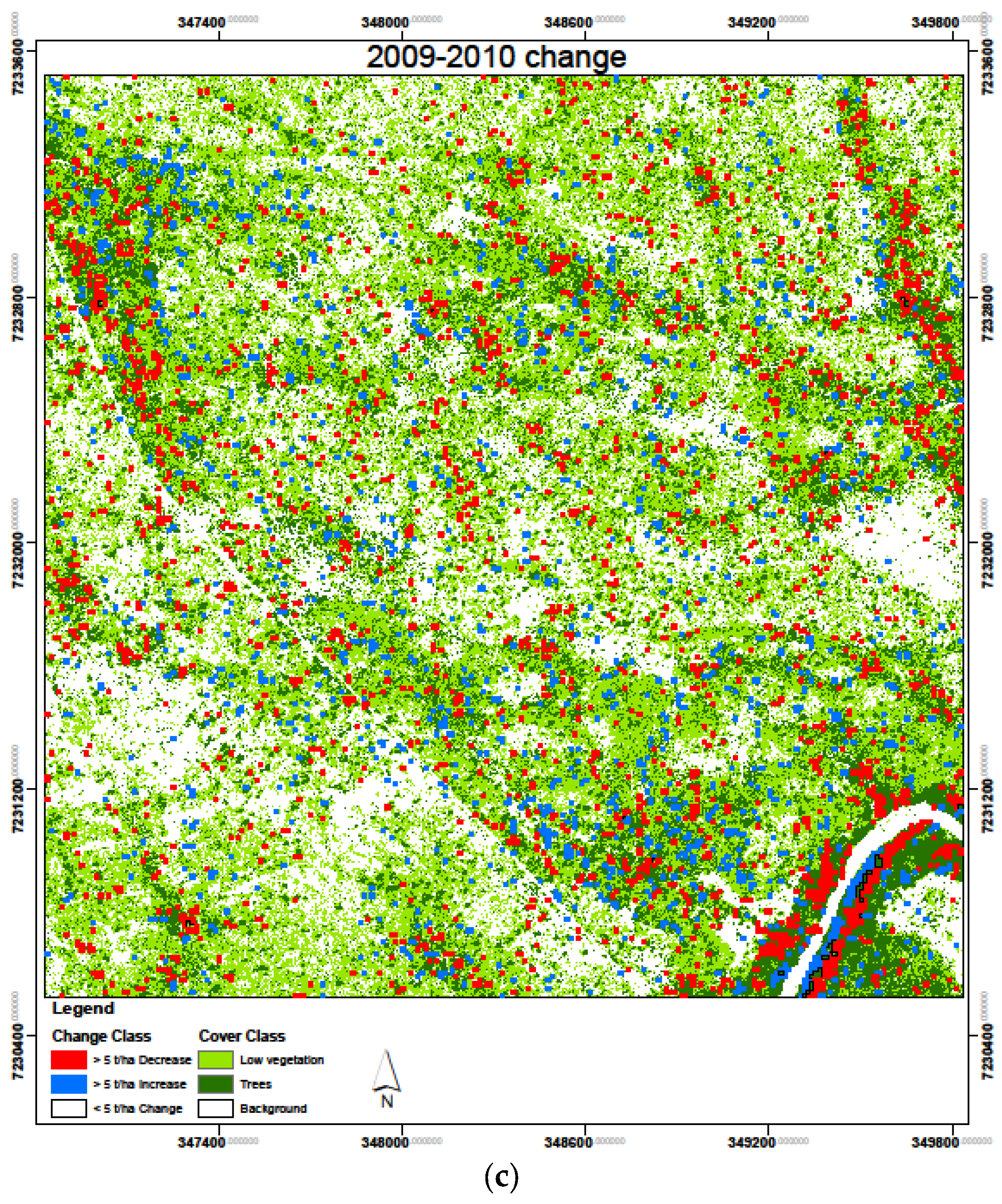
3.4. Biomass Change Detection
3.5. Uncertainty and Error Analysis
4. Discussion
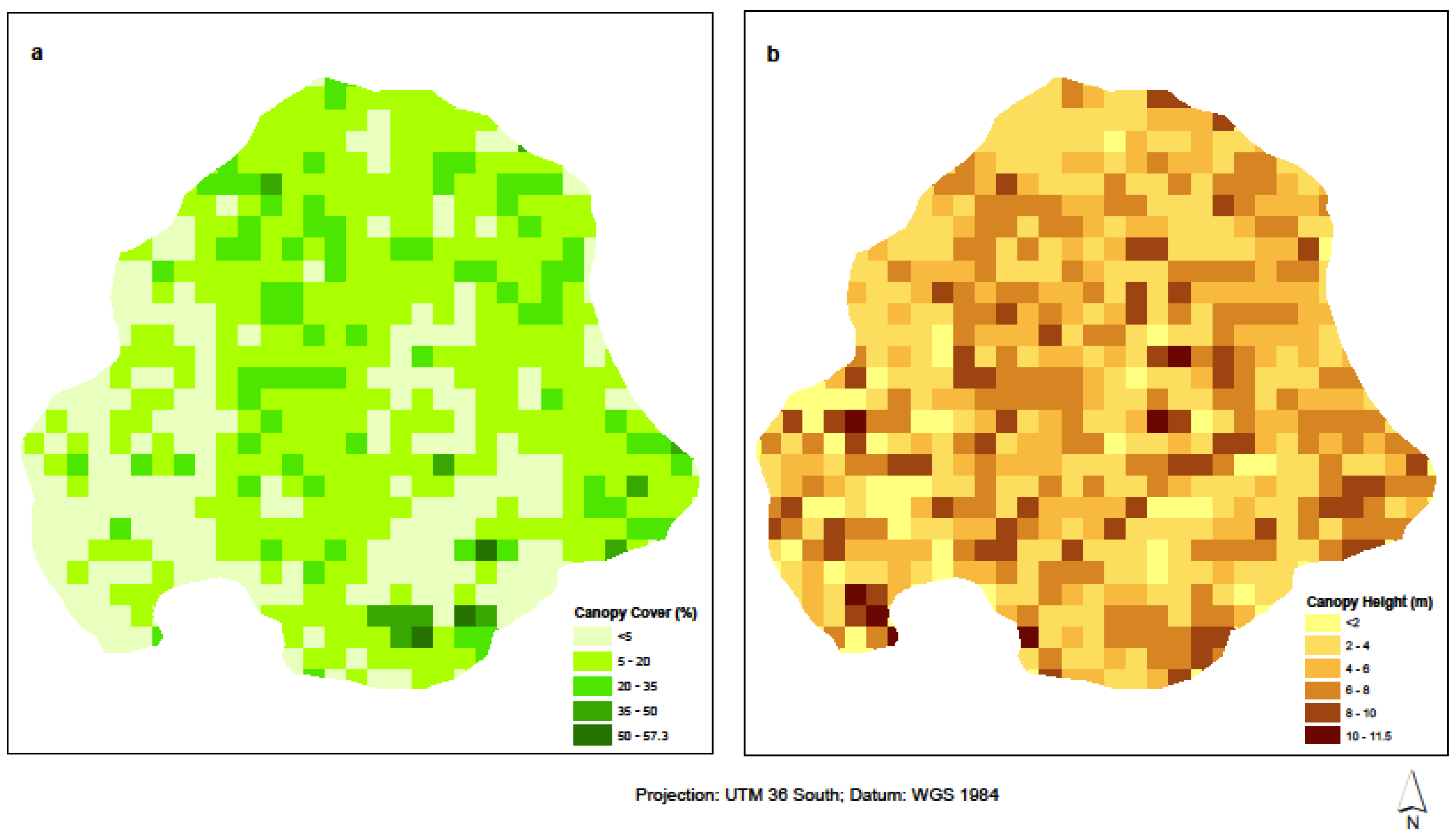
4.1. Distribution of Woody Biomass
4.2. Temporal Dynamics in Woody Biomass
4.3. Uncertainties in Biomass Prediction
5. Conclusions
Acknowledgments
Author Contributions
Conflicts of Interest
References
- Intergovernmental Panel on Climate Change (IPCC). Good Practice Guidance for Land Use, Land-Use Change and Forestry; Glossary 1; IPCC National Greenhouse Gas Inventories Program: Hayama, Japan, 2003. [Google Scholar]
- Gibbs, H.K.; Brown, S.; Niles, J.O.; Foley, J.A. Monitoring and estimating tropical forest carbon stocks: Making REDD a reality. Environ. Res. Lett. 2007, 2, 13. [Google Scholar] [CrossRef]
- Roy, P.S.; Ravan, A.S. Biomass estimation using satellite remote sensing data—An investigation on possible approaches for natural forest. J. Biosci. 1996, 21, 535–561. [Google Scholar] [CrossRef]
- Esser, G. The significance of biospheric carbon pools and fluxes for the atmospheric CO2: A proposal mode structure. Prog. Biometeorol. 1984, 3, 253–294. [Google Scholar]
- Chave, J.; Condit, R.; Aguilar, S.; Hernandez, A.; Lao, S.; Perez, R. Error propagation and scaling for Tropical forest biomass estimates. Philos. Trans. R. Soc. 2004, 359, 409–420. [Google Scholar] [CrossRef] [PubMed]
- Nickless, A.; Scholes, R.J.; Archibald, S. A method for calculating the variance and confidence intervals for tree biomass estimates obtained from allometric equations. Afr. J. Sci. 2011, 107. [Google Scholar] [CrossRef]
- Clark, D.A.; Brown, S.; Kicklighter, D.; Chambers, J.Q.; Thomlinson, J.R.; Ni, J. Measuring net primary production in forests: Concepts and field methods. Ecol. Appl. 2001, 11, 356–370. [Google Scholar] [CrossRef]
- Chave, J.; Andalo, C.; Brown, S.; Cairns, M.A.; Chambers, J.Q.; Eamus, D.; Fölster, H.; Fromard, F.; Higuchi, N.; Kira, T.; et al. Tree allometry and improved estimation of carbon stocks and balance in tropical forests. Oecologia 2005, 145, 87–99. [Google Scholar] [CrossRef] [PubMed]
- Jenkins, J.C.; Chojnacky, D.C.; Heath, L.S.; Birdsey, R.A. National-scale biomass estimatoes for United States tree Species. For. Sci. 2003, 49, 12–35. [Google Scholar]
- Brown, S. Measuring carbon in forests: Current status and future challenges. Environ. Pollut. 2002, 116, 363–372. [Google Scholar] [CrossRef]
- Saatchi, S.S.; Harris, N.L.; Brown, S.; Lefsky, M.; Mitchard, E.T.A.; Salas, W.; Zutta, B.R.; Buermann, W.; Lewis, S.L.; Hagen, S.; et al. Benchmark map of forest carbon stocks in tropical regions accross three continents. Proc. Natl. Acad. Sci. USA 2011, 108, 9899–9904. [Google Scholar] [CrossRef] [PubMed]
- Baccini, A.; Laporte, N.; Goetz, S.J.; Sun, M.; Dong, H. A first map of tropical Africa’s above-ground biomass derived from satellite imagery. Environ. Res. Lett. 2008, 3, 045011. [Google Scholar] [CrossRef]
- Lefsky, M.A.; Harding, D.J.; Keller, M.; Cohen, W.B.; Carabajal, C.C.; Espirito-Santo, F.D.B.; Hunter, M.O.; Oliveria, R., Jr. Estimates of forest canopy height and aboveground biomass using ICESat. Geophys. Res. Lett. 2005, 32, 1–4. [Google Scholar] [CrossRef]
- Colgan, M.S.; Asner, G.P.; Levick, S.R.; Martin, R.E.; Chadwick, O.A. Topo-edaphic controls over woody plant biomass in South African savannas. Biogeosciences 2012, 9, 1809–1821. [Google Scholar] [CrossRef] [Green Version]
- Colgan, S.M.; Asner, G.P.; Swemmer, T. Harvesting tree biomass at the stand-level to assess the accuracy of field and airborne biomass estimation in savannas. Ecol. Appl. 2013, 5, 1170–1184. [Google Scholar] [CrossRef]
- Korpella, I. Individual tree measurements by use of digital aerial photogrammetry. In Silva Fennica Monographs 3; The Finnish Forest Research Institute: Helsinki, Finland, 2004. [Google Scholar]
- Abraham, J.; Adolt, R. Stand Heights Estimations Using Aerial Images and Laser Datasets; Workshop on 3D RS in Forestry: Vienna, Austria, 2006; Volume 2a, pp. 24–31. [Google Scholar]
- Browning, D.M.; Archer, S.R.; Byrne, A.T. Fiel validation of 1930s aerial photography: What are we missing? J. Arid Environ. 2009, 73, 844–853. [Google Scholar] [CrossRef]
- Raumonen, P.; Casella, E.; Calders, K.; Murphy, S.; Akerblom, M.; Kaasalainen, M. Massive-scale tree modelling from TLS data. ISPRS Ann. 2015, 189, 25–27. [Google Scholar] [CrossRef]
- Tilly, N.I. Terrestrial Laser Scanning for Crop Monitoring-Capturing 3D Data of Plant Height for Estimating Biomass at Field Scale. Ph.D. Thesis, University of Köln, Köln, Germany, 2015. [Google Scholar]
- Kandrot, S.M. Coastal Monitoring: A New Approach. Department of Geography, Cork University, Ireland. Available online: http://research.ucc.ie/journals/chimera/2013/00/kandrot/09/en (accessed on 20 June 2016).
- Resop, J.P.; Hession, W.C. Terrestrial laser scanning for monitoring streambank retreat: Comparison with traditional surveying techniques. J. Hydraul. Eng. 2010, 136, 794–798. [Google Scholar] [CrossRef]
- Stanley, T. Assessment of FARO 3D Focus Laser Scanner for forest Inventory. Bachelor’s Thesis, University of Southern Queensland, Toowoomba, Australia, 2013. [Google Scholar]
- Calders, K.; Newnham, G.; Burt, A.; Murphy, S.; Raumonen, P.; Herold, M.; Culvenor, D.; Avitabile, V.; Disney, M.; Armston, J.; et al. Nondestructive estimates of aboveground biomass using terrestrial laser scanning. Methods Ecol. Evol. 2015, 6, 198–208. [Google Scholar] [CrossRef]
- Hackenberg, J.; Wassenberg, M.; Spiecker, H.; Sun, D. Non destructive methods for biomass prediction combining TLS derived tree volume and wood density. Forests 2015, 6, 1274–1300. [Google Scholar] [CrossRef]
- Li, S.; Dragicevic, S.; Castro, F.A.; Sester, M.; Winter, S.; Coltekin, A.; Pettit, C.; Jiang, B.; Haworth, J.; Stein, A.; et al. Geospatial big data handling theory and methods: A review and research challenges. ISPRS J. Photogramm. Remote Sens. 2016, 115, 119–133. [Google Scholar] [CrossRef] [Green Version]
- Liu, J.; Li, J.; Li, W.; Wu, J. Rethinking big data: A review on the data quality and usage issues. ISPRS. J. Photogramm. Remote Sens. 2016, 115, 134–142. [Google Scholar] [CrossRef]
- Warmink, J. Vegetation Density Measurements Using Parallel Photography and Terrestrial Laser Scanning. A Pilot Study in the Duursche en Gamerensche Waard. Master’s Thesis, Department of Geography of Utretch University, Utretch, The Netherlands, 2012. [Google Scholar]
- Rees, W.G. Physical Principles of Remote Sensing, 2nd ed.; Cambridge University Press: Cambridge, UK, 2001; pp. 109–133. [Google Scholar]
- Mitchard, E.T.A.; Saatchi, S.S.; Woodhouse, I.H.; Nangendo, G.; Ribeiro, N.S.; Williams, M.; Ryan, C.M.; Lewis, S.L.; Feldpausch, T.R.; Meir, P. Using satellite radar backscatter to predict above-ground woody biomass: A consistent relationship across four different Africa landscapes. Geophys. Res. Lett. 2009, 36, 1–6. [Google Scholar] [CrossRef]
- Woodhouse, I.H. Introduction to Microwave Remote Sensing; Taylor and Francis: London, UK, 2006; pp. 93–149. [Google Scholar]
- Ryan, C.M.; Hill, T.; Woollen, E.; Ghee, C.; Mitchard, E.; Cassels, G.; Grace, J.; Woodhouse, I.H.; Williams, M. Quantifying small-scale deforestation and forest degradation in African woodlands using radar imagery. Glob. Chang. Biol. 2012, 18, 243–257. [Google Scholar] [CrossRef]
- Le Toan, T.; Beaudoin, A.; Riom, J.; Guyon, D. Relating forest biomass to SAR data. IEEE Trans. Geosci. Remote Sens. 1992, 30, 403–411. [Google Scholar] [CrossRef]
- Antonarakis, A.S.; Saatchi, S.S.; Chazdon, R.L.; Moorcroft, P.R. Using Lidar and radar measurement to constrain predictions of forest ecosystem structure and function. Ecol. Appl. 2011, 21, 1120–1137. [Google Scholar] [CrossRef] [PubMed]
- Treuhaft, R.N.; Chapman, B.D.; dos Santos, J.R.; Goncalves, F.G.; Dutra, L.V.; Graca, P.M.L.A.; Drake, J.B. Vegetation profiles in tropical forests from multibaseline interferometric synthetic aperture radar, field, and lidar measurements. J. Geophys. Res. 2009, 114, 1–16. [Google Scholar] [CrossRef]
- Wijaya, A.; Susanti, A.; Liesenberg, V.; Wardhana, W.; Yanto, E.; Soeprijadi, D.; Mcfarlane, C.; Qomar, N. Leaf area index and biomass assessment over tropical peatland forest ecosystem using ALOS Palsar and ENVISAT ASAR data. In Proceedings of the 5th International Workshop on Science and Applications of SAR Polarimetry and Polarimetric Interferometry (ESRIN), Frascati, Italy, 24–28 January 2011.
- Carreiras, J.M.B.; Vasconcelos, M.J.; Lucas, R.M. Understanding the relationship between aboveground biomass and ALOS PALSAR in the forests of Guinea-Bisau (West Africa). Remote Sens. Environ. 2012, 121, 426–442. [Google Scholar] [CrossRef]
- Adler, D.; Synnott, T.J. Permanent Sample Plot Techniques for Mixed Tropical Forest; Tropical Forest Papers; Oxford Forestry Institute: Oxford, UK, 1992; Volume 25. [Google Scholar]
- Urbazaev, M.; Thiel, C.; Mathieu, R.; Naidoo, L.; Levick, S.R.; Smit, I.P.J.; Asner, P.G.; Schmullius, C. Assessment of the mapping of fractional woody cover in southern African savannas using multi-temporal and polarimetric ALOS PALSAR L-band images. Remote Sens. Environ. 2015, 166, 138–153. [Google Scholar] [CrossRef]
- Kutsch, W.L.; Freibauer, A.; Brümmer, C.; Higgins, S.; Schmullius, C.; Thiel-Clemen, T.; Scholes, R.J.; Archibald, S.; Kirton, A.; Walker, S.; et al. Adaptive Resilience of Southern African Savannas (ARS AfricaE) Proposal Call; German Federal Ministry of Education and Research (BMBF): Bonn, Germany, 2012; pp. 2–3. [Google Scholar]
- Scholes, R.J.; Gureja, N.; Ginannecchinni, M.; Dovie, D.; Wilson, B.; Davidson, N.; Piggott, K.; McLoughlin, C.; van der Velde, K.; Freeman, A.; et al. The environmental and vegetation of the flux measurement site near Skukuza, Kruger National Park. Koedoe 2001, 44, 73–83. [Google Scholar] [CrossRef]
- Kutsch, W.L.; Hanan, N.; Scholes, B.; McHugh, I.; Kubheka, W.; Eckhardt, H.; Williams, C. Response of Carbon fluxes to water relations in a savanna ecosystem in South Africa. Biogeoscience 2008, 5, 1797–1808. [Google Scholar] [CrossRef]
- Scholes, R.J.; Archer, S.R. Tree-grass interactions in savannas. JSTOR Annu. Rev. Ecol. Syst. 1997, 28, 517–544. [Google Scholar] [CrossRef]
- Merbold, L.; Ardö, J.; Arneth, A.; Scholes, R.J.; Nouvellon, Y.; de Grandcourt, A.; Archibald, S.; Bonnefond, J.M.; Boulain, N.; Brueggemann, N.; et al. Precipitation as driver of carbon fluxes in 11 African ecosystems. Biogeosciences 2009, 6, 1027–1041. [Google Scholar] [CrossRef]
- Woodward, F.I.; Lomas, M.R. Simulating vegetation processes along the Kalahari Transect. Glob. Chang. Biol. 2004, 10, 383–392. [Google Scholar] [CrossRef]
- Hüttich, C.; Herold, M.; Wegmann, M.; Cord, A.; Strohbach, B.; Schmullius, C.; Dech, S. Assessing effects of temporal compositing and varying observation periods for large-area land cover mapping in semi-arid ecosystems: Implications for global monitoring. Remote Sens. Environ. 2011, 115, 2445–2459. [Google Scholar] [CrossRef]
- Gesner, U.; Machwitz, M.; Conrad, C.; Dech, S. Estimating the fractional cover of growth forms and bare surface savannas. A multi resolution approach based on regression tree ensambles. Remote Sens. Environ. 2013, 129, 90–102. [Google Scholar] [CrossRef] [Green Version]
- Moses, A.C.; Mathieu, R.; Asner, G.P.; Naidoo, L.; van Aardt, J.; Ramoelo, A.; Debba, P.; Wessels, K.; Main, R.; Smit Izak, P.J.; et al. Mapping tree species composition in Southern African savannas using integrated airborne spectral and LiDAR system. Remote Sens. Environ. 2012, 125, 214–226. [Google Scholar]
- Mistry, J. World Savannas. Ecology and Human Use; Pearson Education: Harlow, UK, 2000; pp. 1–25. [Google Scholar]
- Scanlon, T.M.; Albertson, J.D. Canopy scale measurements of CO2 and water vapour exchange along a precipitation gradient in Southern Africa. Glob. Chang. Biol. 2004, 10, 329–341. [Google Scholar] [CrossRef]
- Scholes, R.J.; Dowty, P.R.; Caylor, K.; Parsons, D.A.B.; Frost, P.G.H.; Shugart, H.H. Trends in savanna structure and composition along an aridity gradient in the Kalahari. J. Veg. Sci. 2002, 13, 419–428. [Google Scholar] [CrossRef]
- Sankaran, M.; Hanan, N.P.; Scholes, R.J.; Ratnam, J.; Augustine, D.J.; Cade, B.S.; Gignoux, J.; Higgins, S.I.; Le Roux, X.; Ludwig, F.; et al. Determinants of woody cover in African savannas. Nature 2005, 438, 846–849. [Google Scholar] [CrossRef] [PubMed]
- Mograbi, P.J.; Erasmus, B.F.; Witkowski, E.T.F.; Asner, G.P.; Wessels, K.J.; Mathieu, R.; Knapp, D.E.; Martin, R.E.; Main, R. Biomass increase go under cover: Woody vegetation dynamics in South African rangelands. PLoS ONE 2015, 10, e0127093. [Google Scholar] [CrossRef] [PubMed]
- RIEGL VZ 1000 Data Sheet. 2015. Available online: http://www.riegl.com/uploads/tx_pxpriegldownloads/DataSheet_VZ-1000_2015-03-24.pdf (accessed on 7 April 2016).
- Baade, J.; Schmullius, C. TanDEM-X IDEM precision and accuracy assessment based on a large assembly of differential GNSS measurements in Kruger National Park, South Africa. ISPRS J. Photogramm. Remote Sens. 2016, 119, 496–508. [Google Scholar] [CrossRef]
- Isenburg, M. LAStools—Efficient Tools for LiDAR Processing, version 111216; Rapidlasso GmbH: Gilching, Germany, 2016; Available online: http://lastools.org (accessed on January–June 2016).
- Khosravipour, A.; Skidmore, A.K.; Isenburg, M.; Wang, T.; Hussin, Y.A. Generating pit-free canopy height models from airborne Lidar. Photogramm. Eng. Remote Sens. 2014, 80, 863–872. [Google Scholar] [CrossRef]
- Lim, K.; Treitz, P.; Baldwin, K.; Green, J. Lidar remote sensing of biophysical properties of tolerant northern hardwood forests. Can. J. Remote Sens. 2003, 29, 658–678. [Google Scholar] [CrossRef]
- Ben-Arie, J.R.; Hay, G.J.; Powers, R.P.; Castilla, G.; St-Onge, B. Developing of a pit filling algorithm for LIDAR canopy height models. Comput. Geosci. 2009, 35, 1940–1949. [Google Scholar] [CrossRef]
- American Society for Photogrammetry & Remote Sensing (ASPRS). LAS Specification, version 1.4-R6; American Society for Photogrammetry & Remote Sensing: Bethesda, MD, USA, 2011; p. 10. [Google Scholar]
- Naidoo, L.; Mathieu, R.; main, R.; Kleynhaus, W.; Wessels, K.; Asner, G.; Leblon, B. Savanna woody structure modeling and mapping using multi-frequency (X-, C- and L-band) synthetic aperture radar data. ISPRS J. Photogramm. Remote Sens. 2015, 105, 234–250. [Google Scholar] [CrossRef]
- GAMMA Remote Sensing AG. Differential interferometry and geocoding software. In Geocoding and Image Registration Documentation User’s Guide; Gamma, R.S., Ed.; GAMMA Remote Sensing: Gümligen, Switzerland, 2008. [Google Scholar]
- Oliver, C.; Quegan, S. Understanding Synthetic Aperture Radar Images; SciTech Publishing: Raleigh, NC, USA, 2004. [Google Scholar]
- Argenti, F.; Lapini, A.; Alparone, L.; Bianchi, T. A tutorial on speckle reduction in Synthetic Aperture Radar images. IEEE Geosci. Remote Sens. Mag. 2013, 1, 6–35. [Google Scholar] [CrossRef]
- Castel, T.; Beaudoin, A.; Stach, N.; Stussi, N.; Le Toan, T.; Durand, P. Sensitivity of space-borne SAR data to forest parameters over sloping terrain theory and experiment. Int. J. Remote Sens. 2001, 22, 2351–2376. [Google Scholar] [CrossRef]
- Stussi, N.; Beaudoin, A.; Castel, T.; Gigord, P. Radiometric correction of multiconfiguration spaceborne SAR data over hilly terrain. In Proceedings of the 1st International Workshop on Retrieval of Bio- and Geophysical Parameters from SAR Data for Land Applications, Centre National D’etudes Spatiales (CNES), Toulouse, France, 10–13 October 1995.
- Trimble eCognition Trainings. Available online: http://community.ecognition.com/home/training-material (accessed on 10 January 2016).
- Chai, T.; Draxler, R.R. Interactive comment on “Root mean square error (RMSE) or mean absolute error (MAE)?”. Geosci. Model Dev. 2014, 7, 589–590. [Google Scholar]
- Breiman, L.; Friedman, J.H.; Olshen, R.A.; Stone, C.I. Classification and Regression Trees; Taylor & Francis: Belmont, CA, USA, 1984. [Google Scholar]
- Breiman, L. Random Forest. Mach. Learn. 2001, 45, 5–32. [Google Scholar] [CrossRef]
- Liaw, A.; Wiener, M. Classification and regression by random forest. R News 2002, 2–3, 18–22. [Google Scholar]
- Odipo, V.O.; Luck, W.; Berger, C.; Schmullius, C. Savanna fractional cover classification using machine learning. Unpublished work. 2016. [Google Scholar]
- Smit, I.P.J.; Smit, C.F.; Govender, N.; van der Linde, M.; Macfayden, S. Rainfall, geology and landscape position generates large-scale spatiotemporal fire pattern heterogeneity in an African savanna. Ecography 2013, 36, 447–459. [Google Scholar] [CrossRef]
- Scholtz, R.; Kiker, G.A.; Smit, I.P.J.; Venter, F.J. Identifying drivers that influence the spatial distribution of woody vegetation in Kruger National Park, South Africa. Ecosphere 2014, 5. [Google Scholar] [CrossRef]
- Baldeck, C.A.; Colgan, M.S.; Feret, J.B.; Levick, S.R.; Martin, R.E.; Asner, G.P. Lanscape-scale variation in plant community composition of an African Savanna from airborne species mapping. Ecol. Appl. 2014, 24, 84–93. [Google Scholar] [CrossRef] [PubMed]
- Mitchard, E.T.A.; Saatchi, S.S.; Lewis, S.L.; Feldpausch, T.R.; Woodhouse, I.H.; Sonke, B.; Rowland, C.; Meir, P. Measuring biomass changes due to woody encroachment and deforestation/degradation in a forest-savanna boundary region of Central Africa using multi-temporal L-band radar backscatter. Remote Sens. Environ. 2011, 115, 2861–2873. [Google Scholar] [CrossRef]
- Levick, S.R.; Asner, G.P.; Chadwick, O.A.; Khomo, L.M.; Rogers, K.H.; Hartshorn, A.S.; Kennedy-Bowdoin, T.; Knapp, D.E. Regional insight into savanna hydrogeomorphology from termite mounds. Nat. Commun. 2010, 1, 1–7. [Google Scholar] [CrossRef] [PubMed]
- Scholes, R.J.; Walker, B.H. An African Savanna: Synthesis of the Nylsvley Study; Ambridge University Press: Cambridge, UK, 1993. [Google Scholar]
- Banks, D.J.; Griffin, N.J.; Shackleton, C.M.; Mavrandonis, J.M. Wood supply and demand around two rural settlements in a semi-arid savanna. Biomass Bioenergy 1996, 11, 319–331. [Google Scholar] [CrossRef]
- Wessels, K.J.; Colgan, M.S.; Erasmus, B.F.N.; Asner, G.P.; Twine, W.C.; Mithieu, R.; van Aardt, J.A.N.; Fisher, J.T.; Smit, I.P.J. Unsustainable fuelwood extraction from South African savannas. Environ. Res. Lett. 2013, 8, 014007. [Google Scholar] [CrossRef]
- Wilgen, B.W.; Trollope, W.S.W.; Biggs, H.C.; Potgieter, A.L.F.; Brockett, B.H. Fire as a driver of ecosystem variability. In The Kruger Experience. Ecology and Management of Savanna Heterogeniety; Du Toit, J.T., Rogers, K.H., Biggs, H.C., Eds.; Island Press: London, UK, 2003; p. 149. [Google Scholar]
- Asner, G.P.; Vaughn, N.; Smit, I.P.J.; Levick, S. Ecosystem-scale effects of megafauna in African savannas. Ecography 2016, 39, 240–252. [Google Scholar] [CrossRef]
- Sankaran, M.; Ratnam, J.; Hanan, N.P. Tree-grass coexistence in savannas revisited-insights from an examination of assumptions and mechanisms invoked in existing models. Ecol. Lett. 2004, 7, 480–490. [Google Scholar] [CrossRef]


| Laser Wavelength | Near Infrared |
|---|---|
| Scanning method | Rotating multi-facet mirror (V); rotating head (H) |
| Field of view | 100° vertical, 360° horizontal |
| Laser beam divergence | 0.3 mrad |
| Laser beam footprint | 13.5 cm at 450 m, 70 cm at 1400 m * |
| Laser pulse repetition rate | 70–300 kHz |
| Measurement rate | 29,000–122,000/s |
| Scan speed | 3–120 lines/s (V); 0–60°/s (H) |
| Mode | Date | Polarization | Incident Angle (°) | T | F | Season |
|---|---|---|---|---|---|---|
| FBD | 29 September 2010 | HH-HV | 34.3 | 586 | 6680 | DRY |
| FBD | 11 August 2009 | HH-HV | 34.3 | 586 | 6680 | DRY |
| FBD | 23 September 2008 | HH-HV | 34.3 | 586 | 6680 | DRY |
| FBD | 6 August 2007 | HH-HV | 34.3 | 586 | 6680 | DRY |
| DBH (cm) | Height (m) | AGB (kg/Tree) | |
|---|---|---|---|
| Min | 6.4 | 1.5 | 2.9 |
| Median | 35 | 6.2 | 267.1 |
| Mean | 35.2 | 6.2 | 508.1 |
| Max | 105 | 12 | 5825.6 |
| Predictors | RMSE (t/ha) | Mean AGB± σ (t/ha) | Bias | R2 |
|---|---|---|---|---|
| CC | 4.77 | 32.2± 26.73 | 1.27 | 0.91 |
| CH | 2.13 | 34.2 ± 24.43 | −0.57 | 0.47 |
| CCxCH | 2.32 | 34.2 ± 30.78 | −0.62 | 0.99 |
| SAR-HH | 6.7 | 32.2 ± 14.54 | −0.21 | 0.63 |
| SAR-HV | 6.6 | 32.2 ± 14.29 | −0.26 | 0.74 |
| SAR_2007 | 9.3 | 19.92 ± 2.6 | 0.19 | 0.47 |
| SAR_2008 | 3.9 | 20.07 ± 3.0 | 0.4 | 0.5 |
| SAR_2009 | 4.6 | 20.24 ± 4.8 | −0.6 | 0.61 |
| SAR_2010 | 12.7 | 19.72 ± 5.2 | −0.3 | 0.48 |
| Increase (>5 t/ha) | Decrease (>5 t/ha) | <5 t/ha | ||||
|---|---|---|---|---|---|---|
| Area (ha) | % | Area (ha) | % | Area (ha) | % | |
| 2007–2008 | 29.9 | 3.3 | 28.8 | 3.2 | 841.3 | 93.5 |
| 2008–2009 | 28.9 | 3.2 | 29.9 | 3.3 | 841.2 | 93.5 |
| 2009–2010 | 23.1 | 2.6 | 37.3 | 4.1 | 839.6 | 93.3 |
| Average | 27.3 | 3.0 | 32.0 | 3.5 | 840.7 | 93.4 |
© 2016 by the authors; licensee MDPI, Basel, Switzerland. This article is an open access article distributed under the terms and conditions of the Creative Commons Attribution (CC-BY) license (http://creativecommons.org/licenses/by/4.0/).
Share and Cite
Odipo, V.O.; Nickless, A.; Berger, C.; Baade, J.; Urbazaev, M.; Walther, C.; Schmullius, C. Assessment of Aboveground Woody Biomass Dynamics Using Terrestrial Laser Scanner and L-Band ALOS PALSAR Data in South African Savanna. Forests 2016, 7, 294. https://doi.org/10.3390/f7120294
Odipo VO, Nickless A, Berger C, Baade J, Urbazaev M, Walther C, Schmullius C. Assessment of Aboveground Woody Biomass Dynamics Using Terrestrial Laser Scanner and L-Band ALOS PALSAR Data in South African Savanna. Forests. 2016; 7(12):294. https://doi.org/10.3390/f7120294
Chicago/Turabian StyleOdipo, Victor Onyango, Alecia Nickless, Christian Berger, Jussi Baade, Mikhail Urbazaev, Christian Walther, and Christiane Schmullius. 2016. "Assessment of Aboveground Woody Biomass Dynamics Using Terrestrial Laser Scanner and L-Band ALOS PALSAR Data in South African Savanna" Forests 7, no. 12: 294. https://doi.org/10.3390/f7120294