Forest Harvest Patterns on Private Lands in the Cascade Mountains, Washington, USA


1
United States Geological Survey, Western Geographic Science Center, Menlo Park, CA 94025, USA
2
United States Geological Survey, Western Geographic Science Center, Tucson, AZ 85719, USA
3
Emeritus, United States Geological Survey, Western Geographic Science Center, Corvallis, OR 97333, USA
*
Author to whom correspondence should be addressed.
Forests 2017, 8(10), 383; https://doi.org/10.3390/f8100383
Submission received: 16 August 2017
/
Revised: 28 September 2017
/
Accepted: 3 October 2017
/
Published: 7 October 2017
Abstract
:Forests in Washington State generate substantial economic revenue from commercial timber harvesting on private lands. To investigate the rates, causes, and spatial and temporal patterns of forest harvest on private tracts throughout the Cascade Mountains, we relied on a new generation of annual land-use/land-cover (LULC) products created from the application of the Continuous Change Detection and Classification (CCDC) algorithm to Landsat satellite imagery collected from 1985 to 2014. We calculated metrics of landscape pattern using patches of intact and harvested forest in each annual layer to identify changes throughout the time series. Patch dynamics revealed four distinct eras of logging trends that align with prevailing regulations and economic conditions. We used multiple logistic regression to determine the biophysical and anthropogenic factors that influence fine-scale selection of harvest stands in each time period. Results show that private lands forest cover became significantly reduced and more fragmented from 1985 to 2014. Variables linked to parameters of site conditions, location, climate, and vegetation greenness consistently distinguished harvest selection for each distinct era. This study demonstrates the utility of annual LULC data for investigating the underlying factors that influence land cover change.
Keywords:
LCMAP; CCDC; land use; land cover; land change; forest harvest; Cascade Mountains; Washington1. Introduction
1.1. History of Commercial Logging in Washington State
The history of the commercial timber industry in the state of Washington dates back more than 150 years. Historically, much of the logging in Washington has taken place in the Cascade Mountains due to its abundance of softwood conifer forests. Even today, logging of Washington’s forests continues to be an essential part of the regional economy and a major source of wood products produced in the United States.
The first federal logging regulations and large scale privatization of forest lands began in the early 1900s [1]. Prior to the latter half of the 20th century, federal involvement in the restriction of log exports was relatively muted due to the widespread perception of forests as a limitless resource that was useful for driving economic activity [2]. That standpoint changed with the rapid increase of foreign demand for timber after World War II. Growing concern about the depletion of domestic stocks ultimately resulted in the Department of the Interior and Related Agencies Appropriations Act of 1973, which introduced a near-total ban on the export of unprocessed logs from federal lands west of the 100th meridian in the contiguous United States [2,3]. The Forest Resources Conservation and Shortage Relief Act of 1990 further banned unprocessed timber exports from state-owned forests in the same geographical region, except for selected species and grades [2,4].
Other laws were introduced to address growing conflicts between proponents of conserving intact Pacific Northwest (PNW) forests as biodiversity reserves and those in favor of maximizing revenue opportunities. The most far-reaching legislation was the 1994 Northwest Forest Plan (NWFP) [5], which set forest management policies for more than 9.7 million ha of federal forestland in the PNW and northern California [6] and reduced federal harvest projections by 80% [7]. Increasingly, regulators have also broadened economic and environmental policies to cover private forests. For example, Washington’s Timber Excise Tax was enacted in 1971 to tax timber harvested on private lands (excluding tribal lands), and amended in 1982 to include timber harvested on state and federal lands [8]. Similarly, revisions to the Washington State Forest Practices Rules (Title 222 WAC) in 1999 and 2006 led to stricter harvest laws in non-federal forests where logging could impair stream quality [9,10]. Contemporary forest practices continue to be shaped by federal and state regulations and private land management. Despite a tightening of regulatory oversight over time, timber harvesting on private lands remains relatively unencumbered compared to the forestry practices on federal and state lands.
1.2. Understanding Rates and Patterns of Forest Disturbance
Understanding current rates and patterns of forest disturbance is necessary for monitoring and predicting the degree of forest cover loss, fragmentation, and ecological change across a range of geographic scales. These assessments are critical for land managers charged with balancing the economic and environmental consequences of timber harvest. Researchers continue to wrestle with the question of how best to acquire accurate, timely, and consistent overviews of forest change, condition, and extent. Field collection of data can be a viable monitoring technique over large extents (e.g., the US Forest Service’s Forest Inventory and Analysis (FIA) program) but such studies are designed to compile national-scale statistics rather than capture local land change dynamics [11]. Increasingly, aerial and satellite imagery are the preferred tools for informing large-scale monitoring of landscape change [12]. Imagery from the Landsat series of satellites provides a multi-decade record of repeatable, mid-resolution (30 m) measurements that are suitable for detecting land cover change and tracking forest trends at broad spatial scales [13].
Until recently, most regional-to-national scale studies that rely on Landsat imagery to investigate forest disturbance processes and consequences applied a snapshot approach, in which change is documented at discrete multi-year intervals. The 2008 policy decision by the US Geological Survey to make all new and archived Landsat data freely available to the public has led to scientific analyses that incorporate an increasing number of cloud-free Landsat images in a given time frame [13]. Concomitant advances in computing power and sophistication of image processing platforms have contributed to major gains in change detection and forest mapping efforts (Table 1). For example, the Global Forest Change (GFC) effort maps global forest extent, loss, and gain for the period 2000–2012 at a 30-meter spatial resolution [14]. Forest changes are tracked in every Landsat scene with Google Earth Engine and summarized annually. Similarly, the Continuous Change Detection and Classification (CCDC) algorithm uses all available Landsat data to characterize historical land change at any point across the full Landsat record [15]. Finally, Cohen et al. [16] illustrate the advantages of using the rich Landsat archive and ensembles of change detection approaches to improve forest cover change monitoring.
Monitoring continuous land use/land cover (LULC) change allows researchers to detect and classify land change information at a finer temporal resolution than interval-based approaches, in which the extended periods between image dates may obscure intervening land alterations [17]. Furthermore, change detection on annual time steps is more appropriate for most forest monitoring applications [11]. Perhaps the most critical advantage afforded by the generation of continuous LULC change information is the ability to link land changes to corresponding causal mechanisms. Annual land change estimates can be coupled with temporally dense biophysical, climatic, and anthropogenic datasets to more effectively associate individual events or short-term change drivers with resultant changes on the ground.
The USGS Land Change Monitoring Assessment and Projection (LCMAP) initiative is a new effort to develop a land cover mapping and land change detection system using the CCDC algorithm [18,19]. The purpose of LCMAP is to continuously track and characterize changes in land cover, use, and condition at high temporal and spatial resolutions. The derived information will be applied to assessments of historical and future processes of change in order to support decisions relevant to resource management and environmental policy. Using a modified Anderson classification scheme [20] consistent with the Land Cover Trends Project [21], LCMAP will eventually publish wall-to-wall, national-scale maps of annual land cover and land cover change from 1985 onward. This time period coincides with the availability of Landsat Thematic Mapper (TM), Enhanced Thematic Mapper Plus (ETM+), and Operational Land Imaging (OLI) data.
Initial development and testing of CCDC for LCMAP commenced using a pilot scene in Washington (Landsat Path 46, Row 27) that encompasses all or part of three US Environmental Protection Agency level III ecoregions [22]: North Cascades, Cascades, and Eastern Cascades Slopes and Foothills [18]. Forestry represents the most common contemporary land use change in each of these regions [23].
1.3. Understanding the Causes of Forest Change
Incorporating land change information into a historical assessment requires an analysis of the factors that influence the rates and patterns of each land change process. In regions such as the Cascades, where forest harvest is the predominant change process, logging rates and spatial patterns vary over time based on timber availability (i.e., supply), domestic and foreign demand, federal, state, and local tax policies, environmental regulations, and individual landholder decisions (Figure 1). Timber supply in the Pacific Northwest can be largely influenced by environmental conditions affecting growing conditions [24]. Timber demand is directly influenced by construction stemming from domestic and international economic and population growth [25]. Cultural influences can shape public attitudes towards land uses such as forest harvest. Public beliefs and behaviors can lead to vastly different outcomes, directly influencing regulatory decisions and/or technological innovations that may stimulate or suppress forest harvest rates [26]. Where sufficient data are available, statistical analyses like linear regression, regression tree applications [27], or logistic regression approaches [28] can be applied to understand how the likelihood of harvest events increases or decreases based on underlying drivers. In recent years, multiple logistic regression (MLOR) has become the favored method for modelling land cover change outcomes [29], and has been applied in numerous forest studies ranging from the potential distribution of forests [30] to deforestation [31].
1.4. Objectives
The objective of this study is to characterize and interpret the patterns of forest disturbances on private lands in the Cascade Mountains, Washington using LCMAP land cover data for the period 1985–2014. Our hypotheses are that the high temporal and spatial resolution of the dataset will allow us to (1) detect and track short-term fluctuations in forest land cover conversion rates and patterns that can be linked to contemporaneous driving forces, and (2) identify the key biophysical parameters that influence forest conversion during periods of consistent timber demand. Within broad ecoregion boundaries, our focus is on timber harvest on private lands given their more elastic response to driving factors compared to the constrained logging practices on federal and state lands. Our overall intent is to determine the facility of the annual LCMAP products for capturing and providing insight into forest cover dynamics, with the goal of extending the analyses to broad-scale investigations of diverse land cover classes across the U.S.
2. Materials and Methods
2.1. Study Area
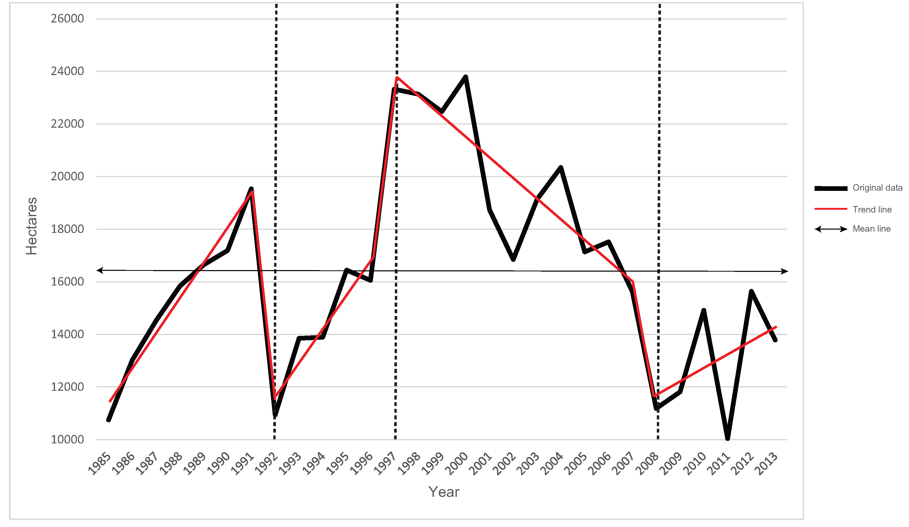
The USGS LCMAP project commenced with a single Landsat scene in Washington State (Path 46, Row 27). To understand the patterns and characteristics of forest disturbances on private lands in this region, we concentrated on three EPA Level III ecoregions in the Cascade Mountains, where forest cover change processes are less complex than in the Puget Lowlands ecoregion to the west. The specific ecoregions included in this study are the North Cascades (EPA Level III ecoregion number 77) and the portions of the Cascades (4) and Eastern Cascades Slopes and Foothills (9) in Washington (Figure 2). Collectively, these ecoregions are characterized by a high degree of topographic relief and a temperate climate with a pronounced west-east moisture gradient; the western region receives approximately twice the annual precipitation as the eastern slopes (20th century mean of 1874 mm vs. 939 mm [32]). The 72.5% of the land cover classified as forest (on the basis of the 2014 LCMAP layer) is predominantly composed of highly productive, coniferous tracts. Douglas-fir (Pseudotsuga menziesii Franco) is the most abundant species on the western side of the Cascades, followed by western red cedar (Thuja plicata Donn ex Don), Pacific silver fir (Abies amabilis Douglas ex Forbes), western hemlock (Tsuga heterophylla Sargent), red alder (Alnus rubra Bongard), and bigleaf maple (Acer macrophyllum Pursh). On the eastern side of the study area, Douglas-fir and ponderosa pine (Pinus ponderosa Douglas ex Lawson) are most common, with some grand fir (Abies grandis Lindley) at higher elevations and oak woodlands (Quercus garryana Douglas ex Hook) in the southeast at lower elevations [23,33].
2.2. Methodological Approach
Our methodological approach consisted of detecting and analyzing forest cover change in annual LCMAP products to isolate forest harvest conversions, quantifying multi-year trends in spatial patterns of forest cover to identify periods of relatively consistent harvest practices, and applying MLOR to identify the main spatial characteristics that determined where forest harvest occurs.
The initial LCMAP product is a 1985–2014 series of annual land cover maps that include a transitional disturbance class (Cover Disturbance Map; hereafter CoverDistMap). An initial assessment of CoverDistMap forest class dynamics in our study area suggests that timber harvest is the leading cause of conversions to the disturbed class, followed by forest fire. Unidirectional changes in forest cover due to development and agriculture are limited in the Cascade Range [23], and were not analyzed in this study. We applied a semi-automated approach to the annual CoverDistMap maps to separate timber harvest from other types of forest disturbances. To identify conversions attributed to fire, an interpreter intersected fire perimeters derived from Monitoring Trends in Burn Severity [34] and USGS Burned Area Essential Climate Variable maps [35] with LCMAP data for the corresponding year. The pixels within each fire perimeter were examined in the CoverDistMap layers immediately prior to and after the fire event (i.e., fire year +/− 1 year) to verify which changes definitively resulted from a burn. Identified pixels were reclassified to a new fire disturbance class. This class is analogous to non-mechanical disturbances mapped by Land Cover Trends [21] and was excluded from subsequent analyses. To focus on forest disturbances, we produced annual from-to conversion maps from the modified CoverDistMap products that were limited to conversions from forest (Year1) to disturbed (Year2). All maps were clipped to a private land mask created by editing a land inventory dataset [36] to exclude areas owned by local, state, or federal entities. For the purposes of this study, private lands are defined as industrial, non-industrial, and tribal lands, which are included because they are often exempt from state and federal regulations. The distinction between industrial forestland, which is owned by forest product companies and managed primarily for timber harvest, and non-industrial forestland is not clearly defined [37]. Since spatially explicit ownership data are not complete for the study area, we group all private lands together without further distinctions. Approximately 27% of the study area, or 1.41 million hectares, is made up of lands defined as private.
2.3. Patch Trend Analysis
We utilized FRAGSTATS [38] landscape metric software to investigate the spatial dynamics of forest and forest-harvest classes on private lands across the study area. In each of the annual 1985–2014 LCMAP maps, we aggregated forest and forest-harvest pixels into respective patches using an 8-cell neighborhood rule; that is, all pixels belonged to a given patch if they were orthogonal or diagonal neighbors with a member of that patch. A qualitative comparison of isolated harvest and forest pixels to aerial photography suggested that single pixels could not be reliably confirmed as accurate, so we removed all patches smaller than 1 hectare [39] to reduce commission errors prior to further processing. For each set of annual class patches we calculated common landscape metrics, including number of patches, mean patch size, total area, mean perimeter/area ratio, and mean Euclidean distance between patches [38].
To identity statistically significant trends, all forest and harvested forest patch metrics were subjected to non-parametric Mann-Kendall tests for monotonic trends [40,41] and Theil-Sen tests [42,43] for the full time series (1985–2014). Monotonic tests are not optimal for time series that include discrete events [44]. Since the abruptness of forest harvest events can be interpreted as breaks, we also tested the time series using Breaks for Additive Season and Trend (BFAST) [45] to identify distinct segments potentially influenced by different spatial or non-spatial drivers (i.e., availability of viable lumber, domestic and international demand, policy, etc.)
2.4. Spatial Statistical Analysis
We performed a spatial statistical analysis to determine the biophysical, climatic, and environmental parameters that differentiate harvested from unharvested forest cover. Sampling of event presence and event absence areas was performed with the goal of establishing a sampling ratio within a range consistent with the literature [46]. Forest harvest (i.e., disturbance) events were randomly sampled from forest-to-disturbance conversion patches in each year (1985–2012). Landsat 7 data were compromised by the sensor’s scan line corrector failure [47], and resulted in insufficient Enhanced Vegetation Index (EVI) data coverage for 2012. Landsat 8 data are incomplete in 2013 due to the satellite launch early that year. Since one of the key covariates is a measure of prior-year greenness, we constrained the time frame to 2012 to match the tenure of Landsat 5 data. To create candidate locations most likely to consist of pixels unaffected by mixed-area issues common at class boundaries [48], we restricted each annual set of patches to those larger than 2 ha and then buffered each area inward by 30 m. A set number of random samples were selected from within all remaining patch areas. Sampling non-changing forest as a proxy for harvest absence required a different process to identify persistent forest pixels in the LCMAP time series. We intersected all annual CoverDistMap layers to identify pixels that were consistently forest from 1985–2014. Random samples were selected from the unharvested patches after filtering for patch size and buffering inward, as was performed with the disturbance patches. The harvested/unharvested points were merged into a single file. To lessen the influence of spatial autocorrelation (spatial dependence across all variables) in the statistical analysis [49,50], we applied a minimum 1-km distribution distance between samples. A total of 2486 samples were obtained, with 952 selected from the unharvested areas and 1534 selected for harvested areas. Approximately 50 random samples were collected for each year in the time series; however, for a few years fewer than 20 harvest samples met our criteria. In the end, the event to non-event ratio varied from 1:1 to 1:9 for each interval.
The dichotomous outcome structure of our dataset (harvested/unharvested) made the choice of a logistic regression analysis appropriate. Logistic regression accepts a binary dependent variable and a set of predictor variables that can include continuous as well as categorical data. Multiple logistic regression analyses are complex, and should be structured to reflect plausible relationships [51]. All statistically significant model variables were evaluated to ensure that each was plausible given the ecological and human dimensions of forest harvest practices. Our pool of potential covariates included factors deemed likely to contribute to favorable forest habitat (i.e., where are conditions most conducive to forest growth?), to influence decisions related to logging logistics (where is it most convenient, feasible, and economical to log?), or to describe the suitability of the trees for harvest (where are the stands appropriate for logging?). We assembled 23 biophysical (soils, elevation, water), climatic (temperature and precipitation), cultural (transportation, population centers, housing density), and vegetation (greenness and stand age) parameters, most of which were adapted from [52] (Table 2).
For the purposes of this study, we treated climatic parameters as static given their long-term influence on tree growth characteristics. Vegetation index metrics were included to highlight differences in greenness characteristics between harvested and unharvested forest cover. While vegetation indices measuring canopy greenness have been applied in select studies to approximate vegetation productivity [53,54], metrics may help identify subtle conditional differences in tree canopy where trees targeted for harvest grow relative to trees that remain uncut, or may merely differentiate forest types preferentially targeted for harvest. In comparison to deciduous stands, coniferous tracts display higher greenness index values in the winter [55], exhibit less variance throughout leaf-on/leaf-off seasons [56,57], and generally appear darker [58,59]. Our hypothesis was that logging areas should consistently reflect these characteristics given the commercial preference for softwood (i.e., coniferous) products: harvest samples would have lower growing season greenness and less variability over the course of a year. We chose to evaluate the Enhanced Vegetation Index (EVI), which was expressly designed to circumvent signal saturation possible with the Normalized Difference Vegetation Index (NDVI) [60]. To create an imagery time series, we assembled all surface reflectance Landsat 5 images over the study area from 1985–2012 in Google Earth Engine [61]. We applied a cloud, shadow, and water mask to each image prior to calculating mean growing season (June–August) EVI, maximum growing season EVI, and annual EVI standard deviation at each harvested/unharvested sample location. To ensure that the vegetation signal was not affected by harvest within or adjacent to each pixel of interest, we associated each point with the EVI metrics from the prior year.
Explanatory variables were extracted to sample points and analyzed using MLOR procedures in statistical software packages SAS version 9.3 (SAS Institute Inc., Cary, NC, USA, 2013) and R version 3.2.3 [62]. Only variables meeting a 95% significance were included in the model selection process. Logistic regression also requires that variables are independent of one another, which can be evaluated using measures of collinearity in the correlation matrix. A correlation threshold of 0.5 was used to identify collinearity between statistically significant variables and remove variables that were not independent.
We performed a stepwise MLOR analysis of harvested forest (presence) and unharvested forest (absence) against the set of explanatory variables. We trained models on 75% of the data and withheld the remaining 25% to test the developed model for goodness of fit and predictive capability. The Wald statistic was used to assess the significance of the individual explanatory variables. Model goodness of fit was evaluated with respect to the receiver operating characteristic (ROC) curve [31] which plots the sensitivity of a test (i.e., the proportion of true observations that are correctly classified as positive) against its specificity (i.e., the proportion of negative observations that are correctly classified as such). The plot is created by varying the threshold value that determines whether probabilities are classified as positive or negative. Models with high discrimination ability will have both high sensitivity and high specificity, translating to a greater amount of area under the curve (AUC). AUC values of 0.5 indicate a random model, in which the explanatory variables do a poor job of informing the predicted observational states.
3. Results
3.1. Patch Trend Analysis
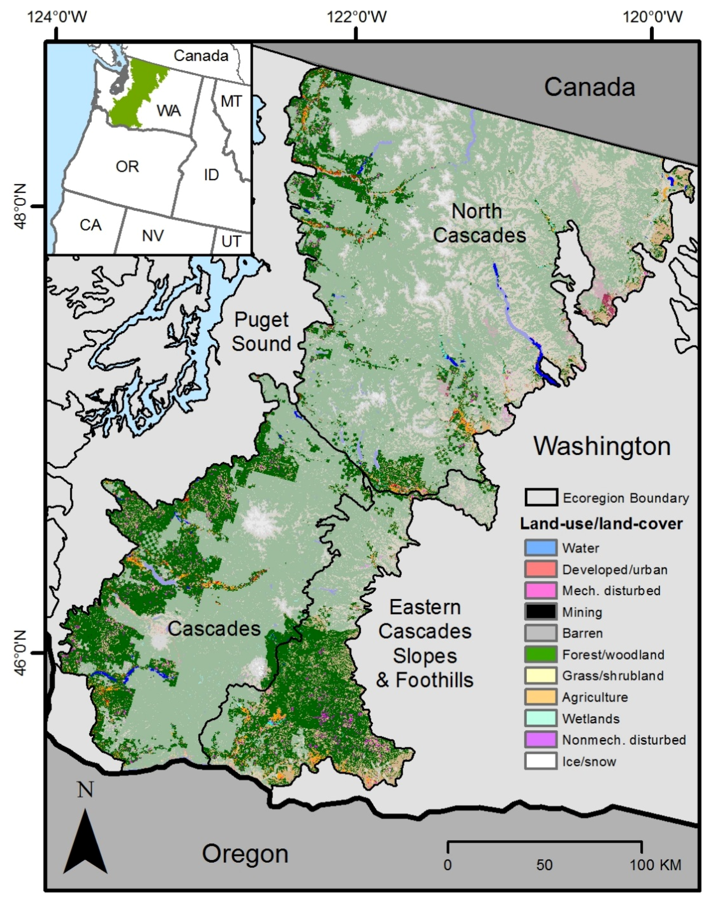
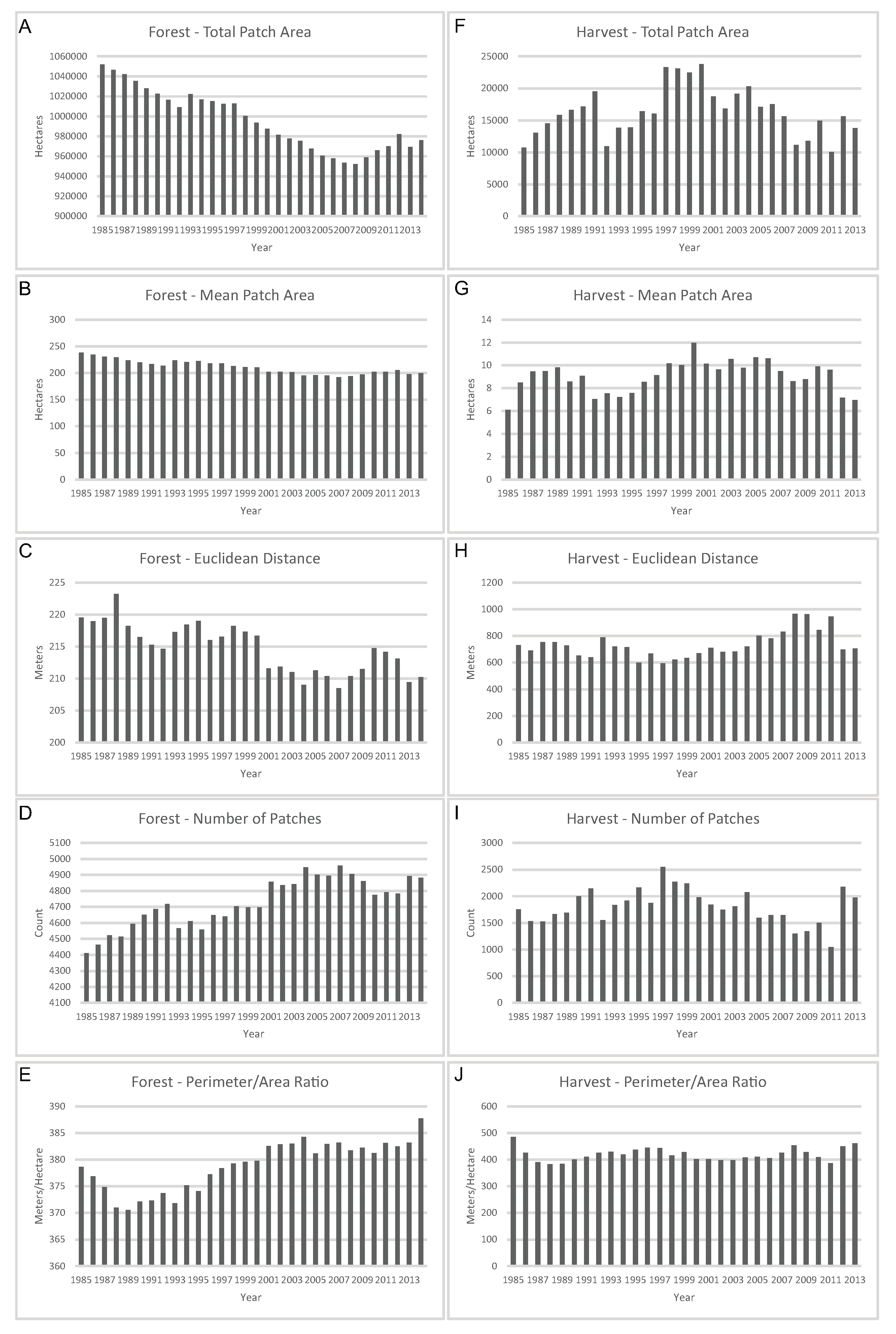
Patch analysis reveals that landscape pattern and structure in the Cascade ecoregions changed over the study time frame, though the individual dynamics of forest and harvest land cover types differed. Between 1985 and 2014, private forests contracted and became significantly more fragmented, as the total forest cover area and mean patch size steadily decreased and the number of discrete patches increased (Figure 3; Table 3) (p ≤ 0.001 for all tested metrics). The landscape shift from relatively fewer, larger patches to more numerous smaller patches is reflected in the declining distance between patches. The increase in forest patch perimeter-to-area ratio suggests that cohesive forest patches also became more irregularly shaped. In contrast, the analysis of harvest patch dynamics yields no statistically significant trends (p > 0.05 for all metrics). Harvest patches exhibit more variability and shorter periods of consistent behavior—increase, decrease, or no trend—throughout the time series, thus justifying the use of BFAST to characterize abrupt changes within the full time period (Figure 4). A general summary of map conversions confirms that harvest is the leading forest conversion driver in the study area. Total patch area for forest to fire and forest to developed conversions average 600 hectares and <100 hectares per year, respectively. By comparison, filtered forest harvest conversions total 16,300 hectares per year on average.
3.2. Multiple Logistic Regression
Although the general suite of variables in the MLOR analysis was consistent—only 10 of the 23 input variables were significant in at least one test—the combinations of significant factors in each time period varied (Table 4). The most consistent variables were July Maximum Temperature (JulyMax) and Standard Deviation Greenness (EVI_stddev), which were significant in all tests, and Distance to Cities 25,000 or more (DistCity25) and National Elevation Dataset (NED), which were significant in all but one test. Distance to Streams (DistStream), Compound Topographic Index (CTI), Soil Moisture Content (Hydric), and Slope were significant in 3 of the 5 different time periods, while Stand Age was a factor in 2 time periods, and Maximum Greenness (EVI_max) was only significant in one. Coefficient estimates and Wald Chi scores also share considerable similarities among the 5 models presented.
The AUC values were similarly variable. The first (1985–1991) and last (2008–2011) time periods returned the highest AUC scores of 0.769 and 0.738, respectively. The 3rd time period model (1997–2007) had the poorest predictive capacity, with an AUC value of 0.638, followed by the overall model with 0.681. All models yield goodness of fit (ROC) performance values that exceed those of a random prediction model.
4. Discussion
4.1. Patch Metrics and Trend Analysis
The combined patch trend results indicate a long-term decrease in forest cover area despite extended periods where forest harvest rates were below the 1985–2014 mean. The sustained decline in forest cover area in this region is primarily a function of harvest, and to a lesser degree, forest disturbance due to fire. Insects and pathogens are also well documented drivers of forest cover change in the region [63,64,65], but this study did not directly measure such changes. Human land-use decisions other than harvest have a minimal direct impact on the amount and structure of private forestland, since conversions to developed parcels or agriculture are low in the Cascade ecoregions. Collectively, these land change processes are altering the landscape in ways that have broad implications for local communities and wildlife. While forest cover often regenerates in the decades following harvest and fire, a steady reduction in the total amount of productive forest will ultimately contribute to declines in private harvest volumes, with attendant disruptions of rural economies that rely on timber and paper industries [64]. The land change dynamics playing out across private forests contrast sharply with the relative stability of intact landscapes managed by the largest landholder in the region, the federal government [66].
The application of BFAST to the total harvested patch area time series identified four distinct periods. Harvest rates were moderate and increasing from 1985 to 1991; lower than average and weakly increasing from 1992 to 1996; highest but decreasing from 1997 to 2007; and once again lower than average and weakly increasing from 2008 to 2012. Private landowners make harvest decisions based on highly diverse and individual reasons, including financial considerations, tract timber age, and personal land preferences. The management of non-industrial private holdings, in particular, is largely uncoordinated and idiosyncratic [67]. The complex mix of influences prevents us from definitively ascribing a specific driving factor to each of the identified periods. Nonetheless, the segmented harvest trends loosely align with predominant economic conditions or regulatory mandates that had documented impacts on forest harvests across the Pacific Northwest.
A series of economic and regulatory factors impacted harvest rates during the 1992 to 1996 interval. Although the era was bookended by a short construction boom in the late 1980s and a larger construction boom in the early 2000s, the number of residential housing units built in the US was at or below the 1965–2015 average (1.44 million housing starts annually) [68]. The abrupt curtailment of log production on federal land by the Northwest Forest Plan [5] led to many mill closures in Washington between 1990 and 1994 [1]. The decline in overall timber industry employment [69] in response to the lowered supply of logs to process may have impacted harvesting in private lands as well by requiring landowners to haul logs farther and reducing the overall processing capacity of the milling sector. Finally, the early 1990s signaled a shift in the US trade balance pertaining to wood products. Over this period, the Pacific Northwest underwent a period of declining timber exports to East Asia [3]. Furthermore, the US also began to import more wood products from Canada (and elsewhere to a lesser degree) than it exported starting in 1993. The negative trade balance increased each year after 1993 and peaked in 2005, as reported by Standard International Trade Classification (SITC) and 1988/1992 Harmonized System (HS) trade classification system data compiled in the United Nations Commodity Trade Statistics database [70]. Forest harvest area, patch size, and patch count were highest from 1997–2007 during a sustained construction boom in the United States [68]. The final break in the BFAST segmentation corresponds well to the recession that began with the collapse of the housing market due to the sub-prime mortgage crisis [71]. International exports of forestry products from the United States increased over the 2008–2012 time period [72]; however, domestic residential construction rates underwent a major decline [68]. In summary, trends in domestic construction demand continue to affect regional logging rates, but international demand for forestry products has emerged as a growing influence on regional logging trends.
4.2. Multiple Logistic Regression
Model variables largely characterize site conditions where softwood conifer species (e.g., Douglas-fir) grow well relative to hardwood deciduous types that are less targeted for harvest. In general, harvest samples are more likely in cooler parts of the study area, where maximum yearly temperatures are relatively low. Harvest samples are also found at relatively drier locations given the lower associated SSURGO soil moisture and Compound Topographic Index (CTI) values. Low CTI values represent places with small catchment capacity while high CTI values represent flatter places including floodplains [73]. Forest harvest may tend to occur less frequently in areas with high CTI based on tree species distributions and environmental regulations in floodplains. Douglas-fir trees, which are prized by loggers, are less abundant on active floodplains and terraces, where deciduous species such as red alder are more plentiful [74,75,76]. In all models, harvested samples have lower EVI standard deviation, which is a characteristic of the more stable growth dynamics of coniferous trees. These findings are generally consistent with past research indicating that deciduous forests in the Pacific Northwest may thrive in locations with more precipitation or wetter soil conditions [76]. A higher distance-to-stream metric for harvest pixels may reaffirm that logging is less common near waterways due to forest composition, but also reflects logging restrictions within riparian buffers. Washington State mandates stringent protections for trees along riparian areas, with logging prohibited or reduced within corridors of different widths from the stream edge [77]. Collectively, these findings largely confirm the results of previous studies conducted in neighboring geographies using different techniques [76,78,79], suggesting that coupling remote sensing and MLOR techniques is a valid method for characterizing growing conditions for conifer-dominated forests.
Elevation and cultural variables included in each model may represent criteria describing the timber selection process. Accessibility and transportation costs directly influence logging activities [80]. The identification of lower elevations and gentler slopes with harvested points may be a function of favorable growing conditions that yield premium timber, but it is more likely that human-use decisions hold sway: trees are more accessible at lower elevations and gentler slopes, and present fewer challenges compared to steep slopes, where specialized cable logging practices are typically required. Accessibility may also explain why harvest samples occur closer to large towns and cities. Processing facilities are often located in larger municipalities, and transportation costs can be minimized.
Interpreting FIA Stand Age across samples may have limits [81], but these data represent the best available proxy for tree age in the study area. In this study, forest stand age is a significant predictive coefficient in the 1985–1991 and 2008–2012 models, in which older trees are more likely to be selected for harvest. The average age of harvest in the random samples is 49 years (1985–1991) and 59 years (2008–2012), which correspond to 40–50 year Douglas-fir clear-cut rotation cycles [82]. In comparison, unharvested forest samples average 48 years. While the inference can be made that unharvested forest samples may skew younger because they include young conifers nearing their cutting rotation age, the aforementioned variables included in the model suggest that these samples include deciduous trees such as red alder and maple trees that live only about 100 years. Only 0.05% of the unharvested samples exceed a 100-year stand age.
5. Conclusions
According to USGS Land Change Monitoring Assessment and Projection (LCMAP) data, more than 70% of the softwood harvest in the Cascade Mountains currently takes place on private lands. With many parts of Washington now used for human settlements and agriculture, and most old growth forests no longer intact, clear cutting and selective harvesting now primarily takes place in smaller and increasingly fragmented tracts of private forest.
To gain a deeper understanding of the rates, causes, and spatial and temporal patterns of forest harvest on private tracts throughout the Cascade Mountains, we decided to undertake a formal analysis of LCMAP data. By successfully resolving annual forest cover dynamics at a 30 m resolution, we not only describe logging rates and patterns for the Cascades Mountains with more detail than ever before, but also demonstrate the potential of annual land cover data for tracking landscape responses to natural, socio-economic, and regulatory external driving forces on a consistent basis. The identification of distinct trends in forest harvesting over time is the first step towards quantifying temporal drivers by identifying periods where influences differ. Segmenting the MLOR process into intervals shows how model variables change over time, and these temporal differences provide insight into shifting site conditions where trees are harvested. Collectively, our research presents an alternative approach to disentangling the site characteristics and human decision-making processes taking place on private forests in the Cascades. While the trend and regression analyses used in this application are not novel concepts, the fact that many of our results can be confirmed with previous studies further demonstrates the utility of LCMAP data for understanding why logging processes take place in specific locations.
The findings presented here represents the first of many land cover investigations in the United States using LCMAP products. As the geographical scope of LCMAP products expands to encompass the continental United States, researchers will have the opportunity to build upon past research on forest dynamics [83] by analyzing the longest annual LULC monitoring effort to date.
Acknowledgments
This research was supported by the USGS Land Change Science and USGS Climate Research and Development programs. We would like to thank Dr. Thomas Loveland (USGS) for contributing the LCMAP maps for these analyses, and Daniel Sorenson (USGS) for editing the land cover maps. We would also like to thank James Vogelmann, Kristi Sayler, and anonymous journal reviewers for their suggestions. Any use of trade, firm, or product names is for descriptive purposes only and does not imply endorsement by the USA Government.
Author Contributions
C.S. and J.W. conceived and designed the experiments; C.S. and J.W. performed the experiments; C.S. and J.W. analyzed the data; J.W. contributed analysis tools; C.S., J.W., and G.G. wrote the paper.
Conflicts of Interest
The authors declare no conflict of interest.
Appendix A
Annual patch statistics and samples of presence and absence used in the multiple logistic regression are provided on USGS Science base. Data can be accessed by searching by article title, author name, or digital object identifier (10.5066/F7X63KWW).
References
- Chiang, C.Y.; Reese, M. Evergreen State: Exploring the History of Washington’s Forests. Available online: https://content.lib.washington.edu/curriculumpackets/Evergreen_State.pdf (accessed on 2 April 2017).
- Lane, C.L. Log export and import restrictions of the U.S. Pacific Northwest and British Columbia: Past and present. USDA For. Ser. Gen. Tech. Rep. 1998, 1, 61. [Google Scholar] [CrossRef]
- Daniels, J.M. The rise and fall of the Pacific Northwest log export market. USDA For. Ser. Gen. Tech. Rep. 2005, 1, 80. [Google Scholar] [CrossRef]
- Gorte, R.W.; Thomas, K.R. Restricting Softwood Log Exports: Policy and Legal Implications. Available online: https://digital.library.unt.edu/ark:/67531/metacrs71/m1/1/high_res_d/93-738_1993Aug13.html#A (accessed on 12 June 2017).
- U.S. Department of Agriculture Forest Service; U.S. Department of the Interior Bureau of Land Management. Record of Decision on Management of Habitat for Late Successional and Old-Growth Forest Related Species within the Range of the Northern Spotted Owl (Northwest Forest Plan); US Government Printing Office: Portland, OR, USA, 1994.
- Kennedy, R.E.; Yang, Z.; Cohen, W.B.; Pfaff, E.; Braaten, J.; Nelson, P. Spatial and temporal patterns of forest disturbance and regrowth within the area of the Northwest Forest Plan. Remote Sens. Environ. 2012, 122, 117–133. [Google Scholar] [CrossRef]
- Bormann, B.T.; Haynes, R.W.; Martin, J.R. Adaptive management of forest ecosystems: Did some rubber hit the road? Bioscience 2007, 57, 186–191. [Google Scholar] [CrossRef]
- Schlosser, W.E.; Baumgartner, D.M.; Hanley, D.P. Forest Land and Timber Excise Taxes in Washington; Pullman: Washington, DC, USA, 1998. [Google Scholar]
- U.S. Fish and Wildlife Service, U.S.; National Marine Fisheries Service; U.S. Environmental Protection Agency, W.S; (Office of the Governor, Department of Natural Resources, Department of Fish and Wildlife, and Department of Ecology); Colville Confederated Tribes and other Washington State Tribes; Washington State Association of Counties; Washington Forest Protection Association; Washington Farm Forestry Association. Forests and Fish Report; Department of Natural Resources: Washington, DC, USA, 1999; p. 173.
- Washington State Department of Natural Resources Forests Practices Program. Final Forest Practices Habitat Conservation Plan; Olympia: Washington, DC, USA, 2005; p. 138.
- Masek, J.G.; Healey, S.P. Monitoring U.S. forest dynamics with Landsat. In Global Forest Monitoring from Earth Observation; Achard, F., Hansen, M.C., Eds.; CRC Press/Taylor & Francis Group: Boca Raton, FL, USA, 2013; pp. 211–228. [Google Scholar]
- Kennedy, R.E.; Townsend, P.A.; Gross, J.E.; Cohen, W.B.; Bolstad, P.; Wang, Y.Q.; Adams, P. Remote sensing change detection tools for natural resource managers: Understanding concepts and tradeoffs in the design of landscape monitoring projects. Remote Sens. Environ. 2009, 113, 1382–1396. [Google Scholar] [CrossRef]
- Wulder, M.A.; Masek, J.G.; Cohen, W.B.; Loveland, T.R.; Woodcock, C.E. Opening the archive: How free data has enabled the science and monitoring promise of Landsat. Remote Sens. Environ. 2012, 122, 2–10. [Google Scholar] [CrossRef]
- Hansen, M.C.; Potapov, P.V.; Moore, R.; Hancher, M.; Turubanova, S.A.; Tyukavina, A.; Thau, D.; Stehman, S.V.; Goetz, S.J.; Loveland, T.R.; et al. High-resolution global maps of 21st-century forest cover change. Science 2013, 342, 850–853. [Google Scholar] [CrossRef] [PubMed]
- Zhu, Z.; Woodcock, C.E. Continuous change detection and classification of land cover using all available Landsat data. Remote Sens. Environ. 2014, 144, 152–171. [Google Scholar] [CrossRef]
- Cohen, W.B.; Healey, S.P.; Yang, Z.; Stehman, S.V.; Brewer, C.K.; Brooks, E.B.; Gorelick, N.; Huang, C.; Hughes, M.J.; Kennedy, R.E.; et al. How similar are forest disturbance maps derived from different landsat time series algorithms? Forests 2017, 8, 98. [Google Scholar] [CrossRef]
- Soulard, C.E.; Wilson, T.S. Recent land-use/land-cover change in the Central California Valley. J. Land Use Sci. 2015, 10, 59–80. [Google Scholar] [CrossRef]
- Pengra, B.; Gallant, A.L.; Zhu, Z.; Dahal, D. Evaluation of the initial thematic output from a continuous change-detection algorithm for use in automated operational land-change mapping by the U.S. Geological Survey. Remote Sens. 2016, 8, 811. [Google Scholar] [CrossRef]
- Zhu, Z.; Gallant, A.L.; Woodcock, C.E.; Pengra, B.; Olofsson, P.; Loveland, T.R.; Jin, S.; Dahal, D.; Yang, L.; Auch, R.F. Optimizing selection of training and auxiliary data for operational land cover classification for the LCMAP initiative. ISPRS J. Photogramm. Remote Sens. 2016, 122, 206–221. [Google Scholar] [CrossRef]
- Anderson, B.J.R.; Hardy, E.E.; Roach, J.T.; Witmer, R.E. A land use and land cover classification system for use with remote sensor data. Geol. Surv. Prof. Pap. 964 1976, 2001, 41. [Google Scholar]
- Loveland, T.R.; Sohl, T.L.; Stehman, S.V.; Gallant, A.L.; Sayler, K.L.; Napton, D.E. A strategy for estimating the rates of recent United States land-cover changes. Photogramm. Eng. Remote Sens. 2002, 68, 1091–1099. [Google Scholar]
- U.S. Environmental Protection Agency. Level III and IV Ecoregions of the Continental United States. Available online: https://www.epa.gov/eco-research/level-iii-and-iv-ecoregions-continental-united-states (accessed on 15 June 2017).
- Sleeter, B.M.; Wilson, T.S.; Acevedo, W. Status and Trends of Land Change in the Western United States—1973 to 2000; U.S. Geological Survey Professional Paper 1794-A; U.S. Geological Survey: Reston, VA, USA, 2012; p. 324.
- Curtis, R.O.; Carey, A.B. Timber supply in the Pacific Northwest: Managing for economic and ecological values in Douglas-fir forest. J. For. 1996, 94, 4–7, 35–37. [Google Scholar]
- Hyde, W.F. Timber Supply, Land Allocation, and Economic Efficiency; Routledge: Abingdon, UK, 1980; p. 224. [Google Scholar]
- Geist, H.J.; Lambin, E.F. Proximate causes and underlying driving forces of tropical deforestation. Bioscience 2002, 52, 143. [Google Scholar] [CrossRef]
- DeFries, R.S.; Rudel, T.; Uriarte, M.; Hansen, M. Deforestation driven by urban population growth and agricultural trade in the twenty-first century. Nat. Geosci. 2010, 3, 178–181. [Google Scholar] [CrossRef]
- Verburg, P.H.; De Koning, G.H.J.; Kok, K.; Veldkamp, A.; Bouma, J. A spatial explicit allocation procedure for modelling the pattern of land use change based upon actual land use. Ecol. Model. 1999, 116, 45–61. [Google Scholar] [CrossRef]
- Serra, P.; Pons, X.; Saurí, D. Land-cover and land-use change in a Mediterranean landscape: A spatial analysis of driving forces integrating biophysical and human factors. Appl. Geogr. 2008, 28, 189–209. [Google Scholar] [CrossRef]
- Felicísimo, A.M.; Francés, E.; Fernindez, J.M.; González-Díez, A.; Varas, J. Modeling the potential distribution of forests with a GIS. Photogramm. Eng. Remote Sens. 2002, 68, 455–461. [Google Scholar]
- Schneider, L.C.; Gil Pontius, R.; Pontius, R.G.J. Modeling land-use change in the Ipswich watershed, Massachusetts, USA. Agric. Ecosyst. Environ. 2001, 85, 83–94. [Google Scholar] [CrossRef]
- National Oceanic and Atmospheric Administration (NOAA); National Center for Environmental Information. Climate Division 6 Precipitation Rankings. Available online: https://www.ncdc.noaa.gov/temp-and-precip/climatological-rankings/ (accessed on 16 June 2017).
- Pater, D.E.; Bryce, S.A.; Thorson, T.D.; Kagan, J.; Chappell, C.; Omernik, J.M.; Azevedo, S.H.; Woods, A.J. Ecoregions of Western Washington and Oregon. Available online: ftp://newftp.epa.gov/EPADataCommons/ORD/Ecoregions/reg10/ORWAFront90.pdf (accessed on 16 June 2017).
- Finco, M.; Quayle, B.; Zhang, Y.; Lecker, J.; Megown, K.A.; Brewer, C.K. Monitoring Trends and Burn Severity (MTBS): Monitoring wildfire activity for the past quarter century using LANDSAT data. In Moving from Status to Trends: Forest Inventory and Analysis Symposium; U.S. Department of Agriculture, Forest Service, Northern Research Station: Newtown Square, PA, USA, 2012; pp. 222–228. [Google Scholar]
- Hawbaker, T.J.; Stitt, S.; Beal, Y.-J.; Schmidt, G.; Falgout, J.; Williams, B.; Takacs, J. Provisional Burned Area Essential Climate Variable (BAECV) Algorithm Description; The United States Department of the Interior: Washington, DC, USA, 2015.
- U.S. Geological Survey Gap Analysis Program (GAP); Protected Areas Database of the United States (PAD-US). Version 1.4; Combined Feature Class; U.S. Geological Survey: Reston, VA, USA, 2016. Available online: https://gapanalysis.usgs.gov/padus/data/download/ (accessed on 4 April 2017).
- Erickson, A.; Rinehart, J. Private Forest Landownership in Washington State. Available online: https://digital.lib.washington.edu/researchworks/bitstream/handle/1773/2233/tp1.pdf (accessed on 23 May 2017).
- McGarigal, K.; Cushman, S.; Ene, E. FRAGSTATS, Version 4; Spatial Pattern Analysis Program for Categorical and Continuous Maps; Oregon State University: Corvallis, OR, USA, 2012. [Google Scholar]
- Kennedy, R.E.; Yang, Z.; Braaten, J.; Copass, C.; Antonova, N.; Jordan, C.; Nelson, P. Attribution of disturbance change agent from Landsat time-series in support of habitat monitoring in the Puget Sound region, USA. Remote Sens. Environ. 2015, 166, 271–285. [Google Scholar] [CrossRef]
- Kendall, M.G. Rank Correlation Methods; Griffin, C., Ed.; John Wiley & Sons: London, UK, 1975. [Google Scholar]
- Mann, H.B. Nonparametric tests against trend. Econometrica 1945, 13, 245–259. [Google Scholar] [CrossRef]
- Sen, P.K. Estimates of the regression coefficient based on Kendall’s Tau. J. Am. Stat. Assoc. 1968, 63, 1379–1389. [Google Scholar] [CrossRef]
- Theil, H. A rank-invariant method of linear and polynomial regression analysis I, II and III. Proc. K. Ned. Akad. Wet. C. 1950, 53, 386–392, 521–525, 1397–1412. [Google Scholar]
- Meals, D.W.; Spooner, J.; Dressing, S.A.; Harcum, J.B. Statistical Analysis for Monotonic Trends, Tech Notes 6, November 2011; U.S. Geological Survey: Fairfax, VA, USA, 2011.
- Verbesselt, J.; Hyndman, R.; Zeileis, A.; Culvenor, D. Phenological change detection while accounting for abrupt and gradual trends in satellite image time series. Remote Sens. Environ. 2010, 114, 2970–2980. [Google Scholar] [CrossRef]
- Heckmann, T.; Gegg, K.; Gegg, A.; Becht, M. Sample size matters: Investigating the effect of sample size on a logistic regression susceptibility model for debris flows. Nat. Hazards Earth Syst. Sci. 2014, 14, 259. [Google Scholar] [CrossRef] [Green Version]
- Storey, J.; Scaramuzza, P.; Schmidt, G.; Barsi, J. Landsat 7 scan line corrector-off gap-filled product development process. Proc. Pecora 2005, 16, 23–27. [Google Scholar]
- Hsieh, P.F.; Lee, L.C.; Chen, N.Y. Effect of spatial resolution on classification errors of pure and mixed pixels in remote sensing. IEEE Trans. Geosci. Remote Sens. 2001, 39, 2657–2663. [Google Scholar] [CrossRef]
- Verburg, P.H.; Soepboer, W.; Veldkamp, A.; Limpiada, R.; Espaldon, V.; Mastura, S.S.A. Modeling the spatial dynamics of regional land use: The CLUE-S model. Environ. Manag. 2002, 30, 391–405. [Google Scholar] [CrossRef] [PubMed]
- Getis, A.; Griffith, D.A. Comparative Spatial Filtering in Regression Analysis. Geogr. Anal. 2002, 34, 130–140. [Google Scholar] [CrossRef]
- Menard, S. Applied Logistic Regression Analysis, 2nd ed.; Sage University Papers Series on Quantitative Applications in the Social Sciences 07-106; Sage: Thousand Oaks, CA, USA, 2001. [Google Scholar]
- Sohl, T.L.; Sleeter, B.M.; Sayler, K.L.; Bouchard, M.A.; Reker, R.R.; Bennett, S.L.; Sleeter, R.R.; Kanengieter, R.L.; Zhu, Z. Spatially explicit land-use and land-cover scenarios for the Great Plains of the United States. Agric. Ecosyst. Environ. 2012, 153, 1–15. [Google Scholar] [CrossRef]
- Sims, D.A.; Rahman, A.F.; Cordova, V.D.; El-Masri, B.Z.; Baldocchi, D.D.; Bolstad, P.V.; Flanagan, L.B.; Goldstein, A.H.; Hollinger, D.Y.; Misson, L.; et al. A new model of gross primary productivity for North American ecosystems based solely on the enhanced vegetation index and land surface temperature from MODIS. Remote Sens. Environ. 2008, 112, 1633–1646. [Google Scholar] [CrossRef]
- Waring, R.H.H.; Coops, N.C.C.; Fan, W.; Nightingale, J.M.M. MODIS enhanced vegetation index predicts tree species richness across forested ecoregions in the contiguous U.S.A. Remote Sens. Environ. 2006, 103, 218–226. [Google Scholar] [CrossRef]
- Delbart, N.; Le Toan, T.; Kergoat, L.; Fedotova, V. Remote sensing of spring phenology in boreal regions: A free of snow-effect method using NOAA-AVHRR and SPOT-VGT data (1982–2004). Remote Sens. Environ. 2006, 101, 52–62. [Google Scholar] [CrossRef]
- Evrendilek, F.; Gulbeyaz, O. Deriving Vegetation Dynamics of Natural Terrestrial Ecosystems from MODIS NDVI/EVI Data Over Turkey. Sensors 2008, 8, 5270–5302. [Google Scholar] [CrossRef] [PubMed]
- Nagai, S.; Saitoh, T.M.; Kobayashi, H. In situ examination of the relationship between various vegetation indices and canopy phenology in an evergreen coniferous forest, Japan. Int. J. Remote Sens. 2012, 1161, 6202–6214. [Google Scholar] [CrossRef]
- Baldocchi, D.; Kelliher, F.M.; Black, T.A.; Jarvis, P. Climate and vegetation controls on boreal zone energy exchange. Glob. Chang. Biol. 2000, 6, 69–83. [Google Scholar] [CrossRef]
- Hall-Beyer, M. Patterns in the yearly trajectory of standard deviation of NDVI over 25 years for forest, grasslands and croplands across ecological gradients in Alberta, Canada. Int. J. Remote Sens. 2012, 33, 2725–2746. [Google Scholar] [CrossRef]
- Huete, A.; Didan, K.; Miura, T.; Rodriguez, E.P.; Gao, X.; Ferreira, L.G. Overview of the radiometric and biophysical performance of the MODIS vegetation indices. Remote Sens. Environ. 2002, 83, 195–213. [Google Scholar] [CrossRef]
- Gorelick, N.; Hancher, M.; Dixon, M.; Ilyushchenko, S.; Thau, D.; Moore, R. Google Earth Engine: Planetary-scale geospatial analysis for everyone. Remote Sens. Environ. 2017. [Google Scholar] [CrossRef]
- R Core Team. R, version 3.3.2; R Foundation for Statistical Computing: Vienna, Austria, 2016.
- Washington State Department of Natural Resources Washington’s Forests, Timber Supply, and Forest-Related Industries. Available online: http://www.dnr.wa.gov/publications/em_fwfeconomiclow1.pdf (accessed on 16 June 2017).
- Bradley, G.; Boyle, B.; Rogers, L.W.; Cooke, A.G.; Perez-Garcia, J.; Rabotyagov, S. Retention of High-Valued Forest Lands at Risk of Conversion to Non-Forest Uses in Washington State; College of Forest Resources, University of Washington: Seattle, WA, USA, 2009. [Google Scholar]
- Parker, T.J.; Clancy, K.M.; Mathiasen, R.L. Interactions among fire, insects and pathogens in coniferous forests of the interior western United States and Canada. Agric. For. Entomol. 2006, 8, 167–189. [Google Scholar] [CrossRef]
- Butler, B.J.; Swenson, J.J.; Alig, R.J. Forest fragmentation in the Pacific Northwest: Quantification and correlations. For. Ecol. Manag. 2004, 189, 363–373. [Google Scholar] [CrossRef]
- Kittredge, D.B.; Rickenbach, M.G.; Knoot, T.G.; Snellings, E.; Erazo, A. It’s the network: How personal connections shape decisions about private forest use. North. J. Appl. For. 2013, 30, 67–74. [Google Scholar] [CrossRef]
- U.S. Census Bureau Historical Data: New Residential Construction. Available online: https://www.census.gov/construction/nrc/historical_data/index.html (accessed on 15 June 2017).
- Charnley, S.; Donoghue, E.M.; Stuart, C.; Dillingham, C.; Buttolph, L.P.; Kay, W.; McLain, R.J.; Moseley, C.; Phillips, R.H.; Tobe, L. Socioeconomic Monitoring Results. Volume III: Rural communities and economies. Gen. Tech. Rep. PNW-GTR-649. In Northwest Forest Plan—The First 10 years (1994–2003): Socioeconomic Monitoring Results; Charnley, S., Ed.; U.S. Department of Agriculture, Forest Service, Pacific Northwest Research Station: Portland, OR, USA, 2006; p. 206. [Google Scholar]
- World Bank, W.I.T.S. United States Wood Exports and Imports by Country and Region. Available online: http://wits.worldbank.org/CountryProfile/en/Country/USA/Year/2004/TradeFlow/EXPIMP/Partner/all/Product/44–49_Wood# (accessed on 1 June 2017).
- Daniels, J.M. Assessing the lumber manufacturing sector in western Washington. For. Policy Econ. 2010, 12, 129–135. [Google Scholar] [CrossRef]
- U.S. Department of Commerce International Trade Administration State-by-State Exports for a Selected Market. Available online: http://tse.export.gov/tse/TSEReports.aspx?DATA=SED&39.1183579&-77.211762&false (accessed on 23 May 2017).
- Moore, I.D.; Grayson, R.B.; Ladson, A.R. Digital terrain modelling: A review of hydrological, geomorphological, and biological applications. Hydrol. Process. 1991, 5, 3–30. [Google Scholar] [CrossRef]
- Pabst, R.J.; Spies, T.A. Structure and composition of unmanaged riparian forests in the coastal mountains of Oregon, USA. Can. J. For. Res. 1999, 29, 1557–1573. [Google Scholar] [CrossRef]
- Rot, B.W.; Naiman, R.J.; Bilby, R.E. Stream channel configuration, landform, and riparian forest structure in the Cascade Mountains, Washington. Can. J. Fish. Aquat. Sci. 2000, 57, 699–707. [Google Scholar] [CrossRef]
- Waring, R.H.; Franklin, J.F. Evergreen coniferous forests of the Pacific Northwest. Science 1979, 204, 1380–1386. [Google Scholar] [CrossRef] [PubMed]
- Washington State Department of Natural Resources Title 222-30 WAC—Forest practices rules: Timber harvesting. In Washington Forest Practices Rules (Revised 12–06–2010); State of Washington Department of Natural Resources: Washington, DC, USA, 2010; pp. 1–38.
- Beedlow, P.A.; Lee, E.H.; Tingey, D.T.; Waschmann, R.S.; Burdick, C.A. The importance of seasonal temperature and moisture patterns on growth of Douglas-fir in western Oregon, USA. Agric. For. Meteorol. 2013, 169, 174–185. [Google Scholar] [CrossRef]
- Zhang, Q.B.; Hebda, R.J. Variation in radial growth patterns of Pseudotsuga menziesii on the central coast of British Columbia, Canada. Can. J. For. Res. 2004, 34, 1946–1954. [Google Scholar] [CrossRef]
- Haynes, R.W. An Analysis of the Timber Situation in the United States: 1989–2040; U.S. Department of Agriculture, Forest Service, Rocky Mountain Forest and Range Experiment Station: Fort Collins, CO, USA, 1990; p. 279.
- Stevens, J.T.; Safford, H.D.; North, M.P.; Fried, J.S.; Gray, A.N.; Brown, P.M.; Dolanc, C.R.; Dobrowski, S.Z.; Falk, D.A.; Farris, C.A.; et al. Average stand age from forest inventory plots does not describe historical fire regimes in ponderosa pine and mixed-conifer forests of western North America. PLoS ONE 2016, 11, e0147688. [Google Scholar] [CrossRef] [PubMed]
- Carey, A.B.; Curtis, R.O. Conservation of biodiversity: A useful paradigm for forest ecosystem management. Wildl. Soc. Bull. 1996, 24, 610–620. [Google Scholar]
- Yang, S.; Mountrakis, G. Forest dynamics in the U.S. indicate disproportionate attrition in western forests, rural areas and public lands. PLoS ONE 2017, 12, e0171383. [Google Scholar] [CrossRef] [PubMed]
Figure 1.
Illustration of factors that may influence forest change over time. Factors may operate simultaneously, functioning either as independent or interconnected processes.
Figure 1.
Illustration of factors that may influence forest change over time. Factors may operate simultaneously, functioning either as independent or interconnected processes.
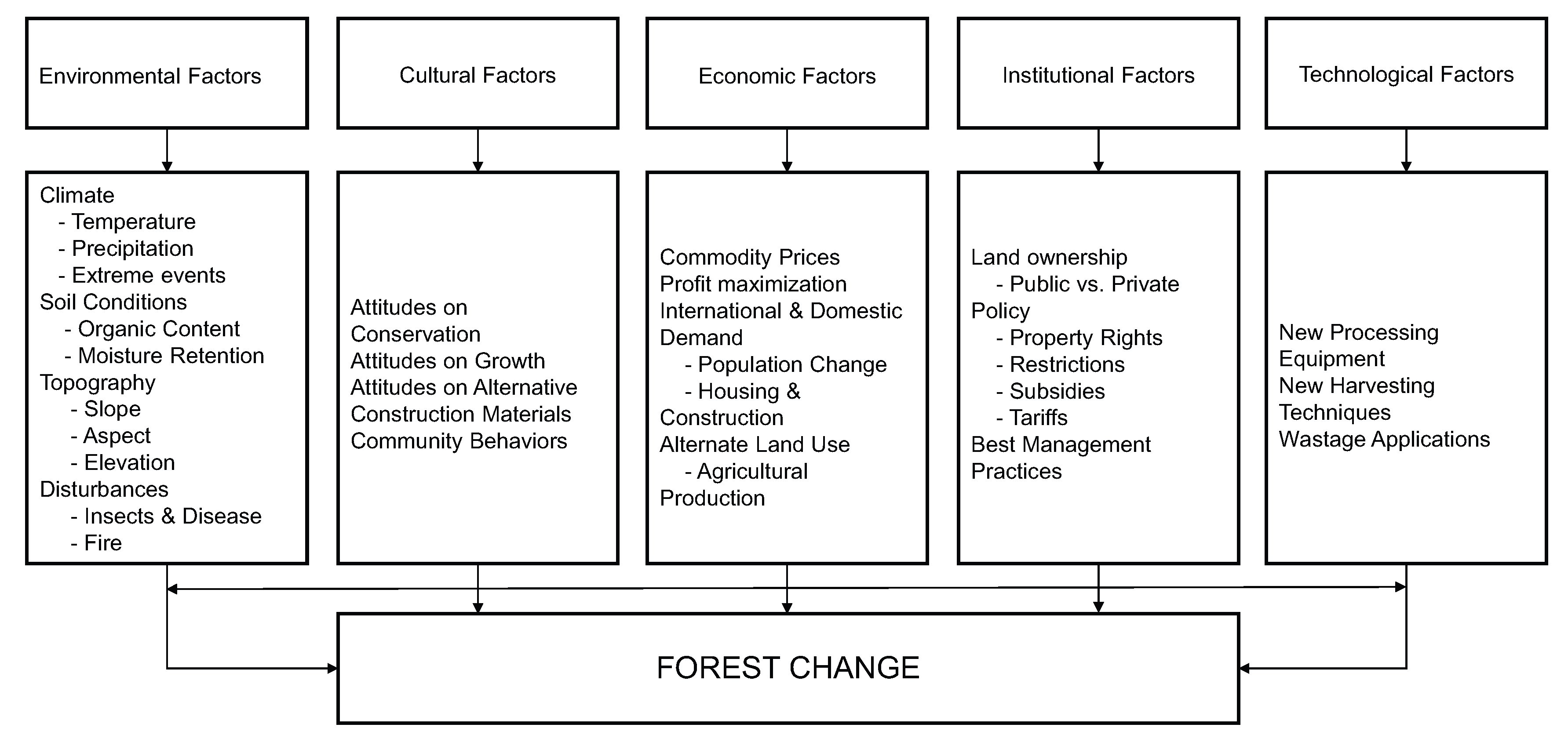
Figure 2.
Study area map showing 2014 LCMAP land use/land cover map for the three Level III ecoregions included in the analysis: North Cascades, Eastern Cascades Slopes and Foothills, and Cascades. Lighter colored areas are owned by local, state, or federal governments, and darker colored areas along the edge of the study area are private lands.

Figure 3.
Annual patch metrics for forest (left, A–E) and forest harvest (right, F–J) classes, 1985–2014. For each set of annual class patches we calculated common landscape metrics, including (in descending order) total class area (sum of all patch areas), mean patch area, mean inter-patch Euclidean distance, number of patches, and mean perimeter/area ratio.

Figure 4.
Output from the BFAST algorithm showing the original time series and the fitted trend component for total harvested patch area. Dashed lines indicate periods within which harvest rates exhibit similarity.
Figure 4.
Output from the BFAST algorithm showing the original time series and the fitted trend component for total harvested patch area. Dashed lines indicate periods within which harvest rates exhibit similarity.

Table 1.
National-scale efforts to map forest change with Landsat imagery. List excludes projects like the National Land Cover Database and Monitoring Trends in Burn Severity that are not solely focused on forest dynamics.
Table 1.
National-scale efforts to map forest change with Landsat imagery. List excludes projects like the National Land Cover Database and Monitoring Trends in Burn Severity that are not solely focused on forest dynamics.
| Dataset | Minimum Mapping Unit | Years Mapped | Source | Number of Landsat Images Used |
|---|---|---|---|---|
| Global Forest Change | 30 m | 2000–2014 | Landsat | Near continuous Landsat time series |
| LANDFIRE vegetation disturbance | 30 m | 1999–2014 | Landsat and cooperator-provided data | Integrated Landsat composites using bi-annual images optimized for change detection |
| North American Forest Dynamics Vegetation Change Tracker | 30 m | 1986–2010 | Landsat | Landsat time-series stacks using one Landsat image per year |
| Web-enabled Data | 30 m | 2006–2010 | Landsat | Near continuous Landsat time series |
Table 2.
Explanatory variables included in multiple logistic regression (MLOR) analysis. All distances are Euclidean measurements (USGS, US Geological Survey; USDA, US Department of Agriculture; SSURGO, Soil Survey Geographic Database; PRISM, Oregon State University PRISM Climate Group).
Table 2.
Explanatory variables included in multiple logistic regression (MLOR) analysis. All distances are Euclidean measurements (USGS, US Geological Survey; USDA, US Department of Agriculture; SSURGO, Soil Survey Geographic Database; PRISM, Oregon State University PRISM Climate Group).
| Input Layer | Source | Description |
|---|---|---|
| Biophysical variables | ||
| Compound Topographic Index | Moore et al. 1991 | Uses slope and runoff to approximate hydrologic catchment |
| National Elevation Dataset | USGS | Cell elevation values |
| Slope | USGS | Derived from National Elevation Dataset |
| Average Water Content | USDA | SSURGO description of water content in soils |
| Soil Organic Content | USDA | SSURGO description of organic content in soils |
| Soil Moisture Content | USDA | SSURGO modified description of soil moisture |
| Distance to Streams | USGS | Distance from closest stream line hydrography feature |
| Distance to Water | USGS | Distance from closest water polygon hydrography feature |
| Climate variables | ||
| January Minimum Temperature | PRISM | The lowest recorded January temperature by location—1971 to 2000 |
| July Maximum Temperature | PRISM | The highest recorded July temperature by location—1971 to 2000 |
| Average Temperature | PRISM | Average annual temperature—1971 to 2000 |
| Average Precipitation | PRISM | Average annual precipitation—1971 to 2000 |
| Cultural variables | ||
| Distance to Railroads | USGS | Distance from closest railroad line feature |
| Distance to Roads | USGS | Distance from closest road line feature |
| Distance to All Cities | USGS | Distance from closest city point feature |
| Distance to Cities (25,000 or more) | USGS | Distance from closest city point feature |
| Distance to Cities (100,000 or more) | USGS | Distance from closest city point feature |
| Housing Density | US Census | 2000 US Census block housing density |
| Population Density | US Census | 2000 US Census block population density |
| Vegetation variables | ||
| Stand Age | USDA | Interpolated forest age from the USDA Forest Inventory and Analysis |
| Maximum EVI Greenness | USGS | Maximum Enhanced Vegetation Index in June–August of year prior to disturbance |
| Mean EVI Greenness | USGS | Mean Enhanced Vegetation Index in June–August of year prior to disturbance |
| Standard Deviation EVI Greenness | USGS | Annual standard deviation of Enhanced Vegetation Index in year prior to disturbance |
Table 3.
Results of Mann-Kendall tests for monotonic trends and Theil-Sen slope estimators of forest and forest harvest patch dynamics. The forest time series is compiled using each annual LULC map, and the forest harvest time series is generated from annual conversion maps. Pixel conversions from forest (Year1) to disturbed (Year2) are categorized as harvest.
| Class | Landscape Metric | Interval Range | Mann-Kendall Trend | Sen’s Slope Estimate | |||||
|---|---|---|---|---|---|---|---|---|---|
| Start | End | Years | Test Z | Significance | Q | Qmin99 | Qmax99 | ||
| Forest | Mean Patch Area | 1985 | 2014 | 30 | −5.32 | p ≤ 0.001 | −1.41 | −1.89 | −1.01 |
| Forest | Total Class Area | 1985 | 2014 | 30 | −5.92 | p ≤ 0.001 | −3591.45 | −4335.00 | −2631.50 |
| Forest | Inter-patch Euclidean Distance | 1985 | 2014 | 30 | −4.57 | p ≤ 0.001 | −0.34 | −0.51 | −0.19 |
| Forest | Number of Patches | 1985 | 2014 | 30 | +4.98 | p ≤ 0.001 | 15.19 | 10.39 | 21.46 |
| Forest | Perimeter/Area Ratio | 1985 | 2014 | 30 | +5.25 | p ≤ 0.001 | 0.47 | 0.27 | 0.65 |
| Harvest | Mean Patch Area | 1985–1986 | 2013–2014 | 29 | +1.29 | ns | 0.04 | −0.05 | 0.13 |
| Harvest | Total Class Area | 1985–1986 | 2013–2014 | 29 | 0.00 | ns | −1.22 | −296.14 | 292.89 |
| Harvest | Inter-patch Euclidean Distance | 1985–1986 | 2013–2014 | 29 | +1.74 | ns | 4.41 | −1.43 | 11.83 |
| Harvest | Number of Patches | 1985–1986 | 2013–2014 | 29 | −0.73 | ns | −5.84 | −30.28 | 17.12 |
| Harvest | Perimeter/Area Ratio | 1985–1986 | 2013–2014 | 29 | +0.84 | ns | 0.66 | −1.26 | 2.10 |
Table 4.
Results of the multiple logistic regression tests in each of the five different time periods. Only variables significant at p ≤ 0.05 are listed.
Table 4.
Results of the multiple logistic regression tests in each of the five different time periods. Only variables significant at p ≤ 0.05 are listed.
| Time Period | AUC | Parameter | Estimate | SE | Significance |
|---|---|---|---|---|---|
| 1985–1991 | 0.769 | Intercept | 7.713 | 1.928 | *** |
| Stand age | 9.898 × 10⁻³ | 767 × 10−3 | ** | ||
| DistCity25 | −1.680 × 10⁻⁵ | 5.734 × 10⁻⁶ | ** | ||
| JulyMax | −0.2.565 | 8.004 × 10⁻² | ** | ||
| CTI | −0.1737 | 6.985 × 10⁻² | * | ||
| NED | −1.728 × 10⁻³ | 4.772 × 10⁻⁴ | *** | ||
| EVI Std | −20.91 | 2.973 | *** | ||
| 1992–1996 | 0.712 | Intercept | 11.69 | 1.419 | *** |
| Diststream | 1.357 × 10⁻⁴ | 3.318 × 10⁻⁵ | *** | ||
| JulyMax | −3.713 × 10⁻¹ | 5.657 × 10⁻² | *** | ||
| CTI | −1.779 × 10⁻¹ | 4.331 × 10⁻² | *** | ||
| NED | −1.805 × 10⁻³ | 3.398 × 10⁻⁴ | *** | ||
| Slope | −5.684 × 10⁻² | 1.391 × 10⁻² | *** | ||
| EVI Stddev | −4.345 | 1.61 | ** | ||
| EVI Max | −4.521 | 7.626 × 10⁻¹ | *** | ||
| 1997–2007 | 0.659 | Intercept | 6.163 | 1.212 | *** |
| DistCity25 | −8.316 × 10⁻⁶ | 2.924 × 10⁻⁶ | ** | ||
| JulyMax | −2.644 × 10⁻¹ | 4.885× 10⁻² | *** | ||
| Hydric | −1.705 × 10⁻² | 5.206 × 10⁻³ | ** | ||
| Slope | −3.598 × 10⁻² | 1.213× 10⁻² | ** | ||
| EVI Stddev | −10.44 | 1.748 | *** | ||
| 2008–2011 | 0.738 | StandAge | 1.724 × 10⁻² | 4.318 × 10⁻³ | *** |
| DistCity25 | −1.513 × 10⁻⁵ | 6.384 × 10⁻⁶ | * | ||
| DistStream | 2.032 × 10⁻⁴ | 5.892 × 10⁻⁵ | *** | ||
| JulyMax | −2.596 × 10⁻¹ | 9.705 × 10⁻² | ** | ||
| NED | −1.171 × 10⁻³ | 5.725 × 10⁻⁴ | * | ||
| EVI Stddev | −9.039 | 3.180 | ** | ||
| 1985–2011 | 0.6814 | Intercept | 7.687 | 8.930 × 10⁻¹ | *** |
| DistCity25 | −6.767 × 10⁻⁶ | 2.157 × 10⁻⁶ | ** | ||
| DistStream | 1.014 × 10⁻⁴ | 2.499 × 10⁻⁵ | *** | ||
| JulyMax | −2.695 × 10⁻¹ | 3.995 × 10⁻² | *** | ||
| Hydric | −1.355 × 10⁻² | 3.627 × 10⁻³ | *** | ||
| CTI | −8.603 × 10⁻² | 2.818 × 10⁻² | ** | ||
| NED | −9.690 × 10⁻⁴ | 2.377 × 10⁻⁴ | *** | ||
| Slope | −3.495 × 10⁻² | 9.655 × 10⁻³ | *** | ||
| EVI_std | −8.577 | 1.162 | *** |
Significance is reported as “***” 0.001 “**” 0.01 “*” 0.05. AUC is the area under the receiver operating curve for each model.
© 2017 by the authors. Licensee MDPI, Basel, Switzerland. This article is an open access article distributed under the terms and conditions of the Creative Commons Attribution (CC BY) license (http://creativecommons.org/licenses/by/4.0/).
Share and Cite
MDPI and ACS Style
Soulard, C.E.; Walker, J.J.; Griffith, G.E. Forest Harvest Patterns on Private Lands in the Cascade Mountains, Washington, USA. Forests 2017, 8, 383. https://doi.org/10.3390/f8100383
AMA Style
Soulard CE, Walker JJ, Griffith GE. Forest Harvest Patterns on Private Lands in the Cascade Mountains, Washington, USA. Forests. 2017; 8(10):383. https://doi.org/10.3390/f8100383
Chicago/Turabian StyleSoulard, Christopher E., Jessica J. Walker, and Glenn E. Griffith. 2017. "Forest Harvest Patterns on Private Lands in the Cascade Mountains, Washington, USA" Forests 8, no. 10: 383. https://doi.org/10.3390/f8100383
Note that from the first issue of 2016, this journal uses article numbers instead of page numbers. See further details here.