Inventory of Close-to-Nature Forests Based on the Combination of Airborne LiDAR Data and Aerial Multispectral Images Using a Single-Tree Approach

Abstract

This study is concerned with the assessment of application possibilities for remote sensing data within a forest inventory in close-to-nature forests. A combination of discrete airborne laser scanning data and multispectral aerial images separately evaluated main tree and forest stand characteristics (i.e., the number of trees, mean height and diameter, tree species, tree height, tree diameter, and tree volume). We used eCognition software (Trimble GeoSpatial, Munich, Germany) for tree species classification and reFLex software (National Forest Centre, Zvolen, Slovakia) for individual tree detection as well as for forest inventory attribute estimations. The accuracy assessment was conducted at the ProSilva demo site Smolnícka Osada (Eastern Slovakia, Central Europe), which has been under selective management for more than 60 years. The remote sensing data were taken using a scanner (Leica ALS70-CM) and camera (Leica RCD30) from an average height of 1034 m, and the ground reference data contained the measured positions and dimensions of 1151 trees in 45 plots distributed across the region. This approach identified 73% of overstory and 28% of understory trees. Tree species classification within overstory trees resulted in an overall accuracy slightly greater than 65%. We also found that the mean difference between the remote-based results and ground data was −0.3% for tree height, 1.1% for tree diameter, and 1.9% for stem volume. At the stand level, the mean difference reached values of 0.4%, 17.9%, and −21.4% for mean height, mean diameter, and growing stock, respectively.

1. Introduction

Unevenly-aged forests are characterized by heterogeneous structures that make ecosystems more stable from both ecological and static viewpoints, as well as more resistant to any damaging agents and destructive factors in the environment. These forests, at the same time, are considered to better fulfill the requirements for multipurpose forest use and the provision of ecosystem services than forests under even-aged rotation forest management (RFM) [1]. Therefore, the importance of unevenly-aged forest management (also known as continuous cover forestry (CCF)) is expected to increase in the future as an alternative to the prevailing RFM.

The concept of close-to-nature forestry developed in Germany from “Naturgemässe Wirtschaftwald”, following “Dauerwald” defined by Möller [2], can be considered a specific CCF system based on the maximal utilization of natural processes to achieve management goals. As summarized by Bauhus et al. [3], close-to-nature forestry is characterized by accepting the species composition adopted at the site, avoiding uncovered areas due to harvest, enhancing forest stability, utilizing natural processes, focusing on the development of individual trees, and forming mixed, unevenly-aged, rich-structured stands. Given the complexity (spatial, age, species heterogeneity) of close-to-nature forests, however, there are some problems related to the lack of adequate inventory and planning tools; this lacking has been the main reason for the limited use of these tools and, in some extreme cases, even the rejection of selective logging in some countries. Therefore, enhanced inventory methods are still needed to obtain spatially explicit information for these kinds of forest ecosystems.

Advanced methods of remote sensing provide an alternative approach to traditional forest inventory and there is potential to meet these monitoring needs, including over heterogeneous forests. Airborne laser scanning (ALS, also called airborne LiDAR) data and aerial images especially provide opportunities to replace or combine terrestrial inventory methods with time-saving and cost-efficient remote sensing solutions. A comprehensive overview of possible remote sensing techniques applicable for resource assessment and monitoring of continuous cover forests was published by Gadow et al. [4]. In this overview, some examples for estimation of stand canopy closure and mapping of forest structure by airborne LiDAR, aerial images or high-resolution satellite data were provided. Recent studies, however, indicate particular problems with the remote-based identification of understory trees, obtaining individual tree attributes from different canopy layers, as well as with species-specific estimations, in more complex stand structures (e.g., [5,6]). One way to overcome these problems is a combination of ALS and image data. However, there are still many research gaps in relation to inventory of close-to-nature forests, and new extensive studies are, therefore, required.

Regardless of forest structure, there are two general approaches to ALS-based forest inventory. The first is the area-based approach (ABA), which uses the statistical correlation between field-measured variables and the metrics of ALS data (e.g., [7,8,9]). The second is individual tree detection (ITD), which is based on the detection of single trees and the extraction or estimation of their attributes (e.g., [10,11,12]). Both ABA and ITD methods have advantages and disadvantages. ABA-based techniques usually provide predictions with small systematic errors. However, the attributes of only the main tree species can be predicted with high accuracy and mainly in heterogeneous stands, whereas the accuracy of the minority species is reduced due to inaccurate species-specific estimations [13]. Several studies related to ABA, therefore, combined information from ALS data with digital aerial images, or applied the nonparametric k-MSN method to more precisely predict species-specific forest variables [14]. On the other hand, ITD-based techniques are suitable for developing species-specific models that can lead to more accurate stand-level estimations, particularly for mixed stands [15]. However, tree-based results are often underestimated due to problems in detecting suppressed and understory trees, especially in stands with a complex forest structure. To overcome this problem, semi-ITD approaches (e.g., [16]) and several techniques for modeling understory trees based on regression estimators (e.g., [17]), probability models (e.g., [18]), and the theoretical distribution or location of small trees (e.g., [19]), as well as the use of a Bayesian inversion framework (e.g., [20]) have been proposed.

Most studies based on ITD, which is the approach used in the present study, have used a canopy height model (CHM) as input for the extraction or derivation of forest inventory attributes (e.g., [21]). These grid-based techniques decrease the size of the datasets, computational time, and the demands on hardware, but they also reduce information regarding the understory. On the other hand, point-based techniques are still computationally demanding. Therefore, techniques that combine some type of digital model and part of point cloud data were developed. There are methods that retrieve points associated with crown segments, which are extracted from the CHM (e.g., [22]), as well as methods that use 3D single-tree modelling and point clouds, which are normalized by using digital terrain model (DTM) (e.g., [23]). These methods, particularly the voxel-based models, represent an efficient trade-off between grid- and point-based techniques. However, external processing of point cloud data is still required [24], or a less demanding method is more suitable for the forestry industry.

The presented fully point-based technique was developed to compensate for the abovementioned drawbacks [25]. First of all, the algorithm uses the complete information contained in the raw point cloud, while the computationally-demanding operations are optimized by tiling and thinning procedures. Thus, although external processing or generation of some type of digital model is not required, computational time is comparable with grid-based techniques and, at the same time, information from the understory is not neglected. Specifically, the initial procedures optimize the number of points via tiling and thinning operations. Subsequently, treetop detection, tree crown delineation, and tree height estimation are performed using the reduced, tiled, and normalized point cloud in the original three-dimensional data structure. The next step requires external inputs, such as the raster layer representing tree species and the allometric model for tree diameter derivation. Finally, based on the detected attributes and external inputs, the algorithm automatically evaluates all tree and stand characteristics. The presented algorithm was integrated into reFLex (remote forestland explorer) software, which was developed by the National Forest Center (Zvolen, Slovakia) for its easy-to-use application by the forestry industry.

The purpose of this study was to assess the possibilities and limitations of the individual tree-detection approach applied by the point-based technique within inventory of close-to-nature forest based on a combination of discrete airborne LiDAR data and multispectral aerial images. There, using all information from point cloud and aerial images should improve the results of the inventory in heterogeneous forests. The main forestry tree and stand characteristics, such as the number, species, height, diameter, and volume, were evaluated separately.

2. Materials and Methods

2.1. Data Sources

The study was conducted in the territory of the ProSilva demo site Smolnícka Osada (48°44′ N, 20°46′ E), where close-to-nature forest management has been applied for more than 60 years (Figure 1). The elevation of the study area reaches intervals of 450–1154 m above sea level (a.s.l.), and the average slope is 40%, which is dominated by northern exposure. The mean annual temperature is 5 °C, and the annual rainfall is 950 mm. Dominant species in the site include European beech (Fagus sylvatica L.), European silver fir (Abies alba Mill.), and Norway spruce (Picea abies L.). Natural regeneration of the forest represents up to 92% of the 2131 ha of the study area.

2.1.1. Ground Reference Data

Ground data were obtained during the leaf-on season in 2014 within circular plots with a radius from 7.5 to 20 m (size of plot was dependent on number of trees). The position of the plot center was measured using the Global Navigation Satellite System (GNSS) and location of each plot was further corrected by visual analysis based on normalized digital surface models and orthophoto images. After manual correction, sub-meter horizontal accuracy was expected for all plots. For the purposes of this study, 45 of 344 reference plots were selected by post-stratification, which was focused on the creation of nine strata (five plots per stratum). The main criteria for stratification were tree species composition and mean diameter. As such, strata were dominated by coniferous trees (C) and broadleaved trees (B), and a mixture of coniferous and broadleaved trees (M) was created. Each stratum was further divided into three development stages defined by mean diameter (C1-3, B1-3, M1-3) (

Table 1. Stratification variables and ground data characteristics.

Stratum: Codes and Criteria		A (ha)	N	hdq (m)	dq (cm)	V (m3)
C	Coniferous ≥ 70%	0.88	419	25.02	30.70	381.70
C1	da < 20 cm	0.15	168	15.63	17.36	34.79
C2	da 20–30 cm	0.29	135	23.94	30.11	107.00
C3	da > 30 cm	0.44	116	31.39	43.73	239.91
B	Broadleaved ≥ 70%	0.90	370	27.37	33.37	465.96
B1	da < 20 cm	0.15	133	18.56	18.24	36.72
B2	da 20–30 cm	0.37	120	27.37	33.76	148.24
B3	da > 30 cm	0.38	117	31.76	44.42	281.00
M	Con. and Broad. < 60%	0.90	362	25.21	31.40	353.52
M1	da < 20 cm	0.16	119	13.84	16.41	19.05
M2	da 20–30 cm	0.31	130	25.26	32.13	127.45
M3	da > 30 cm	0.43	113	30.26	41.09	207.02
Total		2.68	1151	-	-	1201.18
Average		0.89	383.67	25.87	31.82	400.93

Note: A (ha): area in hectare; N: number of trees; h_dq (m): regression height of the tree with the quadratic mean diameter in meters; d_q (cm): quadratic mean diameter in centimeters; V (m³): growing stock in cubic meters; d_a (cm): arithmetic mean diameter in centimeters.

, left section).

Measurements were taken by a mirror compass for tree azimuth relative to plot center and with the Vertex system for tree height, as well as for the distance of trees relative to the plot center. Horizontal and vertical accuracy was expected to be ±1.5 m and ±1.0 m, respectively. Diameter at breast height (DBH) measurements were performed with calipers at the millimeter scale. A total of 1151 trees with a DBH higher than 7 cm were measured for stem position, species, height, diameter, crown length, crown projection, and vitality (Table 1, summary at right).

The tree species composition of the sample was dominated by European silver fir (Abies alba Mill.), with a ratio of 51.9% of total volume, and European beech (Fagus sylvatica L.), with a ratio of 30.3% of total volume. From the perspective of the ratio of the total number of trees, European silver fir reached 30.3%, and European beech reached 41.3% (Figure 2).

2.1.2. Remote Sensing Data

Aerial imaging and airborne laser scanning were carried out simultaneously in September 2014 (leaf-on) using sensors mounted on a Cessna TU206F with an average flight height of 1034 m, field of view (FOV) of 49°, and forward/lateral overlap of 30/60%.

Multispectral aerial images with a dimensions of 9000 × 6732 pixels were acquired using a Leica RCD30 medium-format camera. The available motion range was expected to be ±0.15 mm. In further processing, the images were corrected both for the curvature of the Earth and for atmospheric refraction, orthorectified and mosaicked, which resulted in the creation of natural color orthophoto images (RGB) and color infrared orthophoto images (CIR) with a spatial resolution of 0.2 m and a 16-bit color depth (radiometric calibration was not performed). Considering the parallel acquisition of ALS and image data, using an ALS-based terrain model at a grid resolution of 0.5 × 0.5 m, and precise orthorectification, the geometric accuracy [26] of ortophotos reached value of ±1.1 m.

Laser point clouds were acquired using a Leica ALS 70-CM airborne laser scanner at a 228-kHz pulse rate frequency. The system was configured to record up to five echoes per pulse, and processes were designed to achieve vertical and horizontal accuracies (within one sigma) of 0.15 m and 0.20 m, respectively. The laser data had an average density of laser hits of 4.3 pt/m². In further processing, the point clouds were classified in accordance with the American Society for Photogrammetry and Remote Sensing classes, and noise points were removed using reFLex software [25].

2.2. Remote-Based Forest Inventory

2.2.1. Individual Tree and Tree Height Detection

Treetops, tree crowns, and tree heights were detected using the reFLex algorithm (National Forest Centre, Zvolen, Slovakia), which includes several tree allometry rules on permissible tree heights and crown dimensions to increase the likelihood that real trees are detected. All details on the algorithm are listed in the study of Sačkov et al. [25].

The initial procedures were applied to divide the points into a three-dimensional regular mesh, calculate the absolute height above the ground for each point, and reduce the number of points in the input file by applying a minimum tree height threshold. These operations produced a point cloud that was further used in an iterative search for treetops and tree crowns by using a moving-window analysis. Since there were reasons to assume that a part of the local maxima identified in the previous operation may not be indicative of real treetops, an additional geo-dendrometric (GD) test was applied. The GD test included two steps: first, the height differences between the local maxima located in the testing area were evaluated, and second, the horizontal and vertical distances between all local maxima were evaluated. The horizontal distances were tested to eliminate false treetops situated in the crowns of other trees, and vertical distances were tested to eliminate false treetops situated in the crowns of other trees and to capture trees situated under the canopy. The final procedures were applied to delineate the tree crowns. After the treetop identification and crown delineation phases were completed, tree height was recorded, and the crown coverage was calculated. Stand height evaluation was obtained as the average of the tree data. Finally, the outputs of all procedures were exported to point and polygon vector files in an ESRI shapefile format.

2.2.2. Tree Species Classification

Tree species composition was determined at the level of identified objects and was classified only into general classes of broadleaved and coniferous trees. For this purpose, an object-oriented classification of RGB and CIR orthoimages with a spatial resolution of 0.2 m was used. This classification was processed with the eCognition Developer 8 software (Trimble GeoSpatial, Munich, Germany).

First, multi-resolution segmentation was implemented on the orthophoto images. The estimation of scale parameter (ESP) tool was used for estimating the scale parameters of segmentation. Emphasis was placed more on color than on object shape. Owing to the size and heterogeneity of the study area and the composition of forest stands, the shape factor was set to 0.1, i.e., with low weight, to form the shape of segments; thus, there was greater weight to the spectral homogeneity of pixels. The compactness factor was set to the mean value (0.5), with no enhanced emphasis on the compactness or smoothness of objects.

Second, the samples of three training classes (broadleaved, coniferous, and shadow classes) were chosen by experts randomly based on the visual analysis of orthophoto images. The standard nearest neighbor (SNN) classifier was applied in the classification process. The result was a raster layer representing classes of broadleaved trees, coniferous trees, and shadows. Finally, one of the classification classes was assigned to each delineated tree crown by the reFLex algorithm using zonal statistical functions. Geometrical correspondence between all delineated tree crowns and ortophoto image was secured by manual correction. The result was a vector layer representing the tree crowns with their assigned class as either broadleaved or coniferous trees.

2.2.3. Tree Diameter Derivation

The diameters of the detected trees were derived based on nonlinear regression models. Using ground reference data (randomly selected trees with undamaged single trunks from all of 344 reference plots), the function with the highest correlation between tree height and diameter was selected. The statistical significance of the regression model was assessed using the F-test at a significance level of α = 0.05. We found the exponential function to be most suitable for DBH derivation based on tree height. The final model reached an accuracy of ±19–29% at the tree level, and the coefficient of determination fluctuated from 0.8 to 0.9, with a 95% probability (

Table 2. Regression models used for derivation of tree diameter based on tree height.

Group of Tree Species	Model	n	R	R2	Sd	Sd %	p-Value
Coniferous	d = 7.454 × exp(0.056 × h)	284	0.94	0.89	8.00	19.41	<0.001
Broadleaved	d = 6.857 × exp(0.057 × h)	203	0.89	0.79	8.71	27.89	<0.001

Note: n: sample size; R: correlation coefficient; R²: coefficient of determination; S_d: accuracy of model; S_d %: relative accuracy of model; and p-value: critical value for F-test.

).

For each remotely-detected tree, which included the estimated height (Section 2.2.1) and assigned attribute of tree species classes (Section 2.2.2), the DBH derivation was applied using prepared regression models. Finally, in the cases of systematic errors, the outputs of derivation were corrected using a bias value. Stand diameter evaluation was obtained as the average of the tree data.

2.2.4. Tree Volume Calculation

The volumes of the detected trees were calculated based on models introduced by Petráš et al. [27]; these models are commonly used in Slovakia, and their total accuracy at the tree level reaches ±7–12%. The empirical material for these models includes 1886 beech trees, 1477 fir trees, and 2111 spruce trees from areas across Slovakia and Czechia. The model predictors were tree height and diameter for selected tree species.

For each remotely detected tree, which included the estimated height (Section 2.2.1), assigned attribute of tree species classes (Section 2.2.2), and derived DBH (Section 2.2.3), the volume calculation was applied using the adopted model. As only two classes of tree species were available, the volume functions of the tree species with the highest proportion in the respective growing stock were used as a compromise. For the broadleaved class, the beech function was used; for coniferous, the fir (oldest stands) and spruce functions (youngest stands). Finally, in the cases of systemic errors, the outputs of the calculation were corrected using a bias value. The stand volume calculation was obtained by summing the tree data.

2.3. Accuracy Assessment

2.3.1. Tree Level

An accuracy assessment was carried out by comparing pairs of identical trees measured in the field (GR) and trees derived using remote sensing data (RS). The matching process was conducted by a human interpreter based on normalized digital surface models and orthophoto images. Only detected single treetops within a distance of 5 m from the reference trees and a height difference of ±2 m between the reference trees were candidates for correctly-assigned trees.

Detection rates, especially the extraction rate (ER) (Equation (1)) and matching rate (MR) (Equation (2)), were used to assess the ratio of tree numbers measured on the ground to the remotely-detected tree number with respect to omission and commission errors. The omission error contained the reference trees that could not be linked to any treetop identified using the RS data. The commission error contained the detected treetops that could not be linked to any tree measured in the field. The equations are as follows:

ER = (RS/GR) × 100

(1)

MR = (TP/GR) × 100

(2)

where ER is the extraction rate, MR is the matching rate, RS is the number of remotely detected trees, GR is the number of reference trees, and TP is the true positive.

Assessment of the tree species classification accuracy was done using both the classification error matrix and the calculation of classification accuracy (OA).

In the case of the main tree characteristics (height, diameter, volume), the mean difference (e) was calculated as the average of individual differences and was used as an indicator of systematic errors (i.e., under- or overestimation). First, the shape of the distribution of differences was evaluated using the Shapiro-Wilk W test to allow proper selection of the statistical test (Student or Wilcoxon paired test). The random error component (se) was used to assess the dispersion of differences around the mean difference. Finally, the root mean square error (RMSE) was used to aggregate both the systematic and random error components. The relative e%, se%, and RMSE% were calculated as the ratios of their absolute values and the arithmetic average of the reference data.

2.3.2. Plot Level

The sample size for the accuracy assessment included all trees measured in the field and correctly detected trees based on remote sensing data.

The accuracy assessment focused on the assessment of the effects of forest structure on algorithm performance. The measures of algorithm performance were evaluated against trees per hectare (TPH), stand density index (SDI) (Equation (3)), quadratic mean diameter (QMD) (Equation (4)), and volume per hectare (VPH). In addition, we used a quadratic mean height calculated by regressing on the QMD. The equations are as follows:

$$SDI=TP{H}_k\times {\left(\frac{QM{D}_k}{25}\right)}^{1.605}$$

(3)

$$\mathrm{QMD}=\sqrt{\frac{{\displaystyle \sum _{i=1}^k{d}_i^2}}{N_k}}$$

(4)

where N is number of trees, d is diameter at breast height in centimeters, and i and k are indices for the i-th tree and k-th plot, respectively.

3. Results and Discussion

3.1. Accuracy of Individual Tree Detection

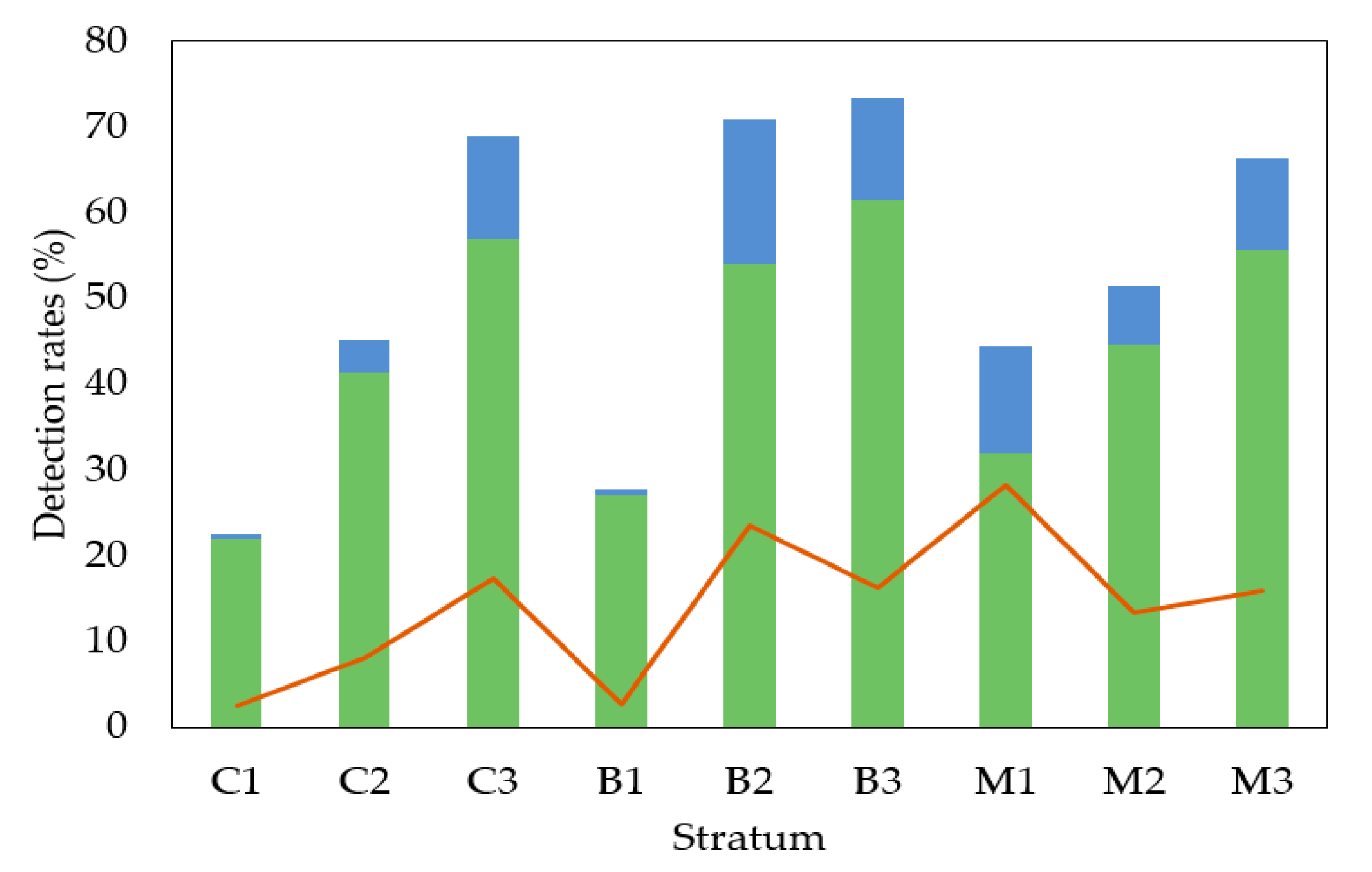
Detection rates for each stratum are shown in Figure 3, and the matching rate for each stratum as well as for each class of tree social status is shown in

Table 3. The overview of matching rates for each stratum and each social position of trees in percentage.

Social Position of Trees	Stratum									Average	Standard Deviation
	C1	C2	C3	B1	B2	B3	M1	M2	M3
Dominant	65.0	83.0	87.8	77.3	93.3	95.7	57.0	85.0	93.8	82.0	13.4
Codominant	57.7	60.0	59.8	61.6	85.0	79.7	48.7	66.6	63.4	64.7	11.2
Intermediate	31.5	19.2	49.7	9.6	54.0	52.3	21.3	24.0	38.0	33.3	16.1
Suppressed	31.6	24.7	32.5	20.4	28.1	8.3	17.7	28.1	6.2	22.0	9.6

. We found matching rates within the interval of 22–62% and a relatively low error of commission that varied between 3% and 28%. The average matching rates for the dominant, co-dominant, intermediate, and suppressed trees were 82%, 65%, 33%, and 22%, respectively.

The best matching rates were achieved within the older forest stands and forest stands where broadleaved trees dominated (tree species composition had no significant impact on accuracy). The results grouped by the social position of trees, however, clearly demonstrate that the decrease in overall matching rates was related to poor detection achieved within understory trees. The differences in matching rates between strata representing an equal development stage (C1 vs. M1, C1 vs. B1, M1 vs. B1, etc.) were not significant, and the effect of tree species composition was marginal in these cases (α = 0.05).

The detection rates in our study are consistent with the results of international research where overall detection fluctuated by approximately 70 ± 25%; these findings are related mainly to the extraction method and the quality of the point clouds [24,28,29]. The structure of the forest stand was also an important parameter, as the dense crown canopy caused most points to be concentrated within the overstory trees. For example, in broadleaved stands, Sačkov et al. [30] detected 66%, 48%, 18%, and 5%; Duncanson et al. [31] detected 70%, 58%, 35%, 21%; and Ferraz et al. [32] detected 99%, 93%, 66%, 15% of the dominant, co-dominant, intermediate, and suppressed trees, respectively. In the case of coniferous stands, the overall accuracy often exceeded levels of 90% [33]. For example, Solberg et al. [34] detected 93% of dominant, 63% of co-dominant, 38% of intermediate, and 19% of suppressed trees within these stands.

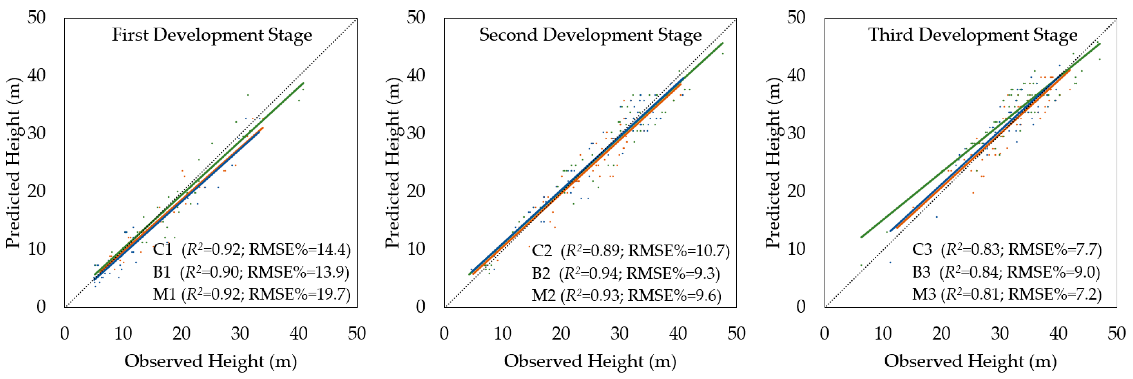
3.2. Accuracy of Tree Height Detection

The accuracy assessment of tree height detection based on the ALS data confirmed systematic errors (α = 0.05). Therefore, all results were corrected with respect to a bias value for different tree height intervals. The results of the accuracy assessment for tree height detection after correction for different tree height intervals are shown in

Table 4. Differences between measured and detected tree heights.

Tree Height Interval (m)	n	e%	se%	RMSE%	Normality Test		Paired Test
					W	p-Value	z	p-Value
All	491	−0.29	12.17	9.74	0.987	<0.001 *	0.259	0.796
≥31	225	−0.01	7.72	7.64	0.968	<0.001 *	0.116	0.908
21–30	138	−0.33	10.70	10.64	0.922	<0.001 *	0.176	0.860
11–20	80	−1.73	17.03	17.10	0.907	<0.001 *	0.249	0.803
≤10	48	−1.36	20.51	19.19	0.969	0.235	0.236	0.814

Note: n: sample size; e%: relative mean error; se%: relative standard deviation of mean error; RMSE%: relative root mean square error; and * null hypothesis was rejected at α = 0.05.

and for each stratum in Figure 4.

We found that tree heights detected and corrected based on the ALS data and bias value provided an output with differences that were not statistically significant relative to the ground data (α = 0.05). Based on the whole-sample size, the remote-based approach underestimated tree height by 0.3 ± 13%, the RMSE% was ±9.7%, and the relationship between the height of the measured and detected trees was very high (R² = 0.89).

Even in this case, a higher accuracy of tree height detection was achieved within the older forest stands, and poor accuracy of heights detected within understory trees caused a decrease in overall precision. On the other hand, differences in the accuracy of tree height detection between the strata representing equal development stages were not significant only for a few pairs of strata. A notable exception was the coniferous and broadleaved stratum in the third development stage (C3 vs. B3), where the difference was significant (α = 0.05). Thus, in older forest stands, the dominance of any group of tree species had an important influence on the accuracy of tree height detection.

Our results confirmed the general statement that tree height is mostly underestimated, but also the most accurate forest inventory attribute within direct estimations based on the ALS data. First, this is an important point because tree height mensuration from the ground is often difficult due to treetops being hidden by the branches of other trees. Second, tree height is useful for the derivation of other forest inventory attributes. In this context, Sibona et al. [35] presented a detailed study where remote-based tree heights and field-based tree heights of a hundred felled trees throughout a coniferous forest were compared using point clouds with a density of 1 pt/m², 5 pt/m², and 10 pt/m². The mean absolute difference ranged from 0.95 to 1.13 m in this study. Similar studies by Brandtberg et al. [36] and Gaveau and Hill [37] that involved deciduous forests have been conducted, where tree heights evaluated based on the ALS data from leaf-off conditions reached an overall standard error of 1.1 m. These authors underestimated shrub canopy height by 0.91 m and main canopy height by 1.27 m. Chávez and Tullis [38] evaluated tree height using ALS data and spectral predictors over full-canopy oak-hickory forests and reported an average error of 1.67–2.99 m, a RMSE of 2.2 m, and a correlation coefficient of 0.42–0.51.

3.3. Accuracy of Tree Species Classification

The overall accuracy of tree species classification for both groups of coniferous and broadleaved trees was relatively low. Classification within overstory trees reached OA at 65.0%. Approximately 83% of all coniferous trees and 33% of all broadleaved trees were correctly identified by the classification (producer’s accuracy (PA)) (

Table 5. Error matrix of tree species classification for overstory trees.

	Reference Data				UA
	Class	Coniferous	Broadleaved	Total	(%)
Classification results	Coniferous	184	83	267	68.91
	Broadleaved	38	41	79	51.90
	Total	222	124	346
PA (%)		82.88	33.06	Overall accuracy	65.03

Note: UA: user accuracy; and PA: producer accuracy.

).

From a stratification perspective, the overall accuracy for strata dominated by broadleaved trees (B1–3) was only 39.9%, while the accuracy results of strata representing coniferous (C1–3) and mixed (M1–3) stands were greater than 63%.

It is evident that the decrease in overall accuracy is related mainly to the classification of broadleaved trees. The broadleaved group was misclassified as a coniferous group, especially in broadleaved strata. High spectral variability occurred in these parts of the area, which was most likely caused by tree health and bidirectional reflectance. Similarly, greater levels of geometric distortion were achieved in that area, probably caused by difficult terrain conditions (differences in elevation). Other more objective causes could have been the social position of trees (broadleaved are mainly within the understory) and shadowed parts of the research area. Therefore, broadleaved trees from the understory were not visible in the remote sensing data or were shadowed, which influenced the spectral values of the respective pixels. Dominant trees may not have been sufficiently illuminated by the sun, and the acquired spectral values of different tree species may also not have been as substantial within the overstory. There, geometric accuracy of ortophoto images partially influenced the results of classification, as well. In this context, the selection of optimal conditions for data acquisition (e.g., weather, season), sensor settings (e.g., FOV, image overlapping), radiometric correction of data, and using a true-ortophoto images or advanced methods for fusion of ALS-image data, resents ways to improve tree species classification accuracy in the future. The use of multiple observations of the same area or aerial and satellite images at different phenological stages would definitely help separate coniferous and deciduous trees, as well.

Information on tree species composition is extremely beneficial, as this information directly describes some qualitative forest characteristics, including structural diversity and habitat quality, and represents an independent variable for estimating many quantitative forest inventory attributes (e.g., tree diameter, tree volume). However, the classification of tree species composition using remote sensing data has proven to be a difficult task. Most studies have estimated tree species using multispectral or hyperspectral aerial imagery by pixel- or object-oriented classification, as described by Ballanti et al. [39]. Methods based on a combination of aerial images and some derivatives from ALS data (e.g., digital models, intensity raster) are also available (as described by Manzanera et al. [40] and Sedliak et al. [41]). Finally, several authors have investigated the potential of discrete or waveform airborne LiDAR data for these purposes, as well as experimentally with spectral airborne LiDAR. There have been a few studies where different forest inventory attributes or variables describing the point cloud were extracted directly from ALS data, such as crown density, crown shape, crown surface texture, echo width, the standard deviation of echo amplitude, the total number of echoes per pulse and received energy from individual peaks, e.g., [42]. Relevant studies focused on using RS data for tree species composition have reported an overall accuracy in the range of 33–95%.

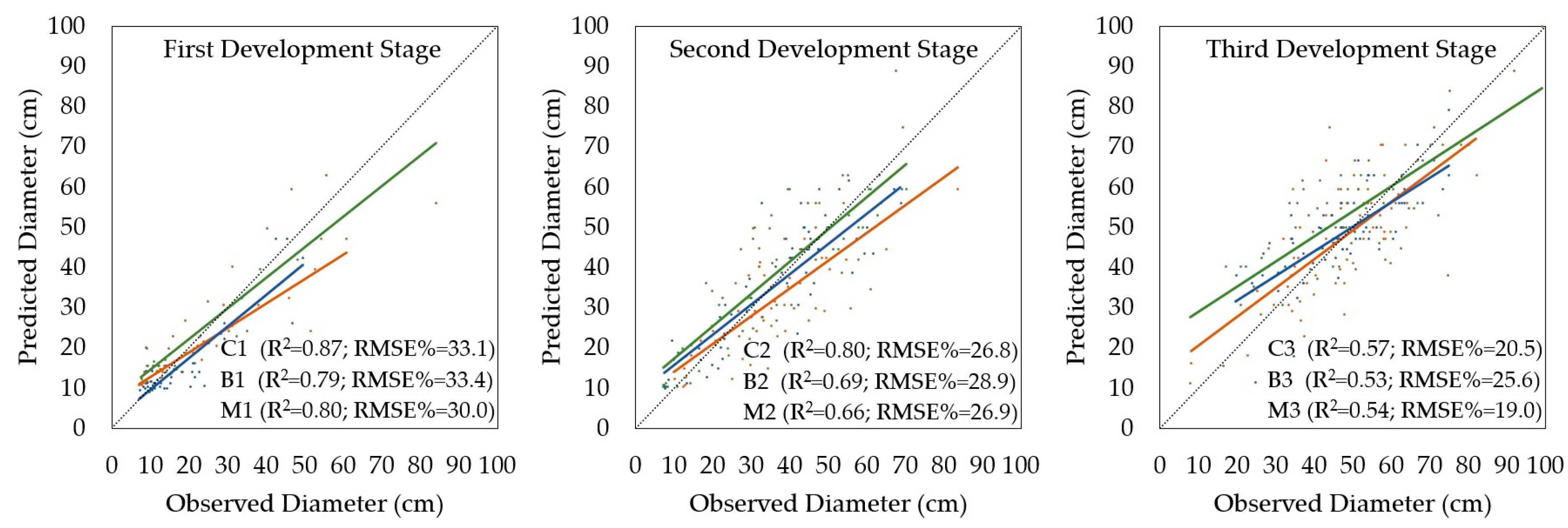
3.4. Accuracy of Tree Diameter Derivation

Tree diameters obtained using the regression model were systematically underestimated in the case of tree height intervals of 21–30 m (α = 0.05). Therefore, the results were corrected with respect to a bias value only for this tree height interval. The results of the accuracy assessment for the tree diameter derivation after correction (tree height interval of 21–30 m) for different tree height intervals are shown in

Table 6. Differences between the measured and derived tree diameters.

Tree Height Interval (m)	n	e%	se%	RMSE%	Normality Test		Paired Test
					W	p-Value	z	p-Value
All	491	1.14	30.56	25.71	0.990	0.001 *	1.210	0.226
≥31	225	2.23	23.06	20.43	0.997	0.947	1.447	0.148
21–30	138	−0.76	33.22	30.09	0.987	0.234	0.050	0.960
11–20	80	−1.09	41.56	37.28	0.965	0.026 *	0.417	0.676
≤10	48	−0.48	30.51	56.88	0.519	<0.001 *	1.908	0.056

Note: n: sample size; e%: relative mean error; se%: relative standard deviation of mean error; RMSE%: relative root mean square error; and * null hypothesis was rejected at α = 0.05.

and for each stratum in Figure 5.

We found that the derived and corrected tree diameters based on the ALS data and bias value provided an output with differences that were not statistically significant relative to the ground data (α = 0.05). Based on the entire sample size, the remote-based approach overestimated the tree diameter by 1.1 ± 31%, the RMSE% was ±25.7%, and the relationship between the diameters of the measured and detected trees was very strong (R² = 0.79).

Regarding the structure of the model, in which tree height is an important parameter, used to predict the tree diameter, the results concerning the best and worst accuracies of diameter derivation were similar as in the case of tree height. However, the significant effect of tree species composition at equal development stages on the accuracy of tree diameter derivation was also confirmed between coniferous and broadleaved strata in the second and third development stages (C2 vs. B2, C3 vs. B3), as well as between broadleaved and mixture strata at the first development stage (B1 vs. M1), where there was a significant difference (α = 0.05). Thus, in the middle and older forest stands, the dominance of any group of tree species had an important influence on the accuracy of tree diameter derivation. In addition, younger broadleaved stands were different from young mixed forest stands with respect to the tree diameter derivation by the proposed model.

The derivation of tree diameters based on the ALS data was undertaken indirectly by model that uses a well-known relationship between tree diameter and tree height. However, as LiDAR metrics are also used on other tree variables, such as crown area, crown height, and crown volume, which were extracted based on the tree detection approach. Furthermore, Prieditis et al. [43] proposed models extended by information on soil type and the age of forest stands. Subsequently, many models have been built on multilinear regressions, least square boosting decision trees, random forests, and ε-support vector regressions. Broad research efforts predicting tree diameters using ALS data by different parametric or nonparametric approaches have achieved an overall RMSE% accuracy that fluctuates from 15% to 23% [44].

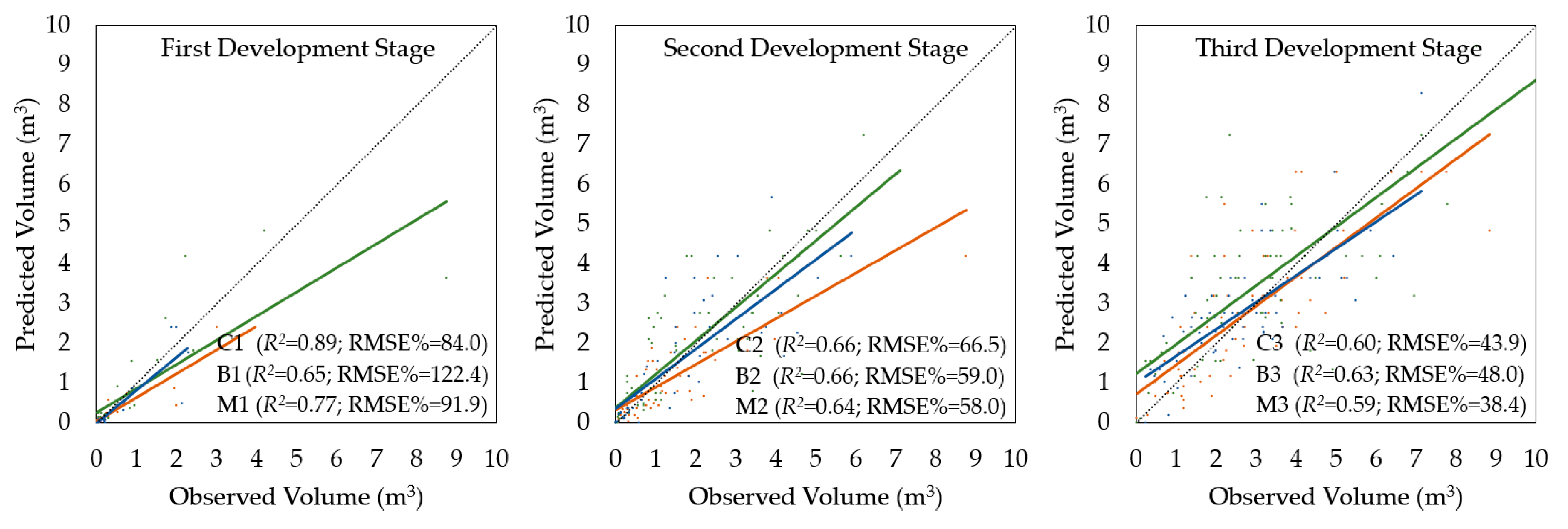
3.5. Accuracy of Tree Volume Calculation

In the case of tree volume, the bias value was not confirmed (α = 0.05); therefore, the results of the calculations were not corrected. The results of the accuracy assessment for the tree volume calculation for different tree height intervals are shown in

Table 7. Differences between the calculated volumes of measured and detected trees.

Tree Height Interval (m)	n	e%	se%	RMSE%	Normality Test		Paired Test
					W	p-Value	z	p-Value
All	491	1.85	91.00	56.08	0.927	<0.001 *	0.688	0.492
≥31	225	2.72	57.40	42.73	0.987	0.043 *	1.035	0.301
21–30	138	−1.59	93.45	68.95	0.948	<0.001 *	0.327	0.744
11–20	80	−6.45	138.21	83.72	0.897	<0.001 *	0.148	0.882
≤10	48	−15.53	96.75	237.69	0.278	<0.001 *	1.849	0.064

Note: n: sample size; e%: relative mean error; se%: relative standard deviation of mean error; RMSE%: relative root mean square error; and * null hypothesis was rejected at α = 0.05.

and for each stratum in Figure 6.

Based on the entire sample size, the remote-based approach overestimated tree diameters by 1.9 ± 91%, the RMSE% was ±56.1%, and the relationship between the diameters of the measured and detected trees was very strong (R² = 0.87).

As expected, the volume equations did not affect the overall interpretation of the results. The oldest forest stands achieved a higher accuracy of tree volume calculation, and the lack of precision increased mainly for understory trees; however, the stem volume of understory trees represented only a small ratio of the overall growing stock. Similar to the previous results, differences in the accuracy of tree volume calculations between strata representing equal development stages were not significant, and the effect of tree species composition in these cases was marginal (α = 0.05).

Tree volume, which is also known as stem volume, represents the final quantitative attribute of forest inventory at the tree level. Since our study was related to the ITD approach, we used an allometric model for tree volume calculation based on tree height and diameter. However, several studies have also used combinations of tree and stand variables. For example, Naesset [45] used percentiles of laser pulse heights and canopy density in a mature forest area and reported a correlation coefficient that ranged from 0.83 to 0.86. The model by Tesfamichael et al. [46] combined LiDAR-derived height variables (stems per hectare as well as stand age), and the level of association between the estimated and observed volume in eucalyptus plantations was relatively high (R² = 0.82–0.94). Furthermore, several models for volume estimation related to the ABA approach have also been reported. In these cases, the forest biophysical variables were regressed against the ALS metrics, and the statistical relationships could be approximated by linear models (e.g., [47]), nonparametric approaches, such as nearest neighbor imputations (e.g., [48]), linear mixed effects models with random stand-level intercepts (e.g., [49]), and Bayesian methods (e.g., [50]). The overall accuracy of both the ITD and ABA approaches within the tree volume calculation based on the ALS data varied from less than 20% to more than 40%, and the mean error was often negative.

3.6. Accuracy at the Plot Level

The proposed remote-based approach evaluated the mean height at 26.0 m by averaging the detected tree heights, the mean diameter at 37.6 cm by averaging the derived tree diameters, and the volume at 955.4 m³ by adding the calculated tree volumes. The smallest differences with the ground data reached values of 0.4%, 17.9%, and −21.4% for the mean height, mean diameter, and growing stock, respectively.

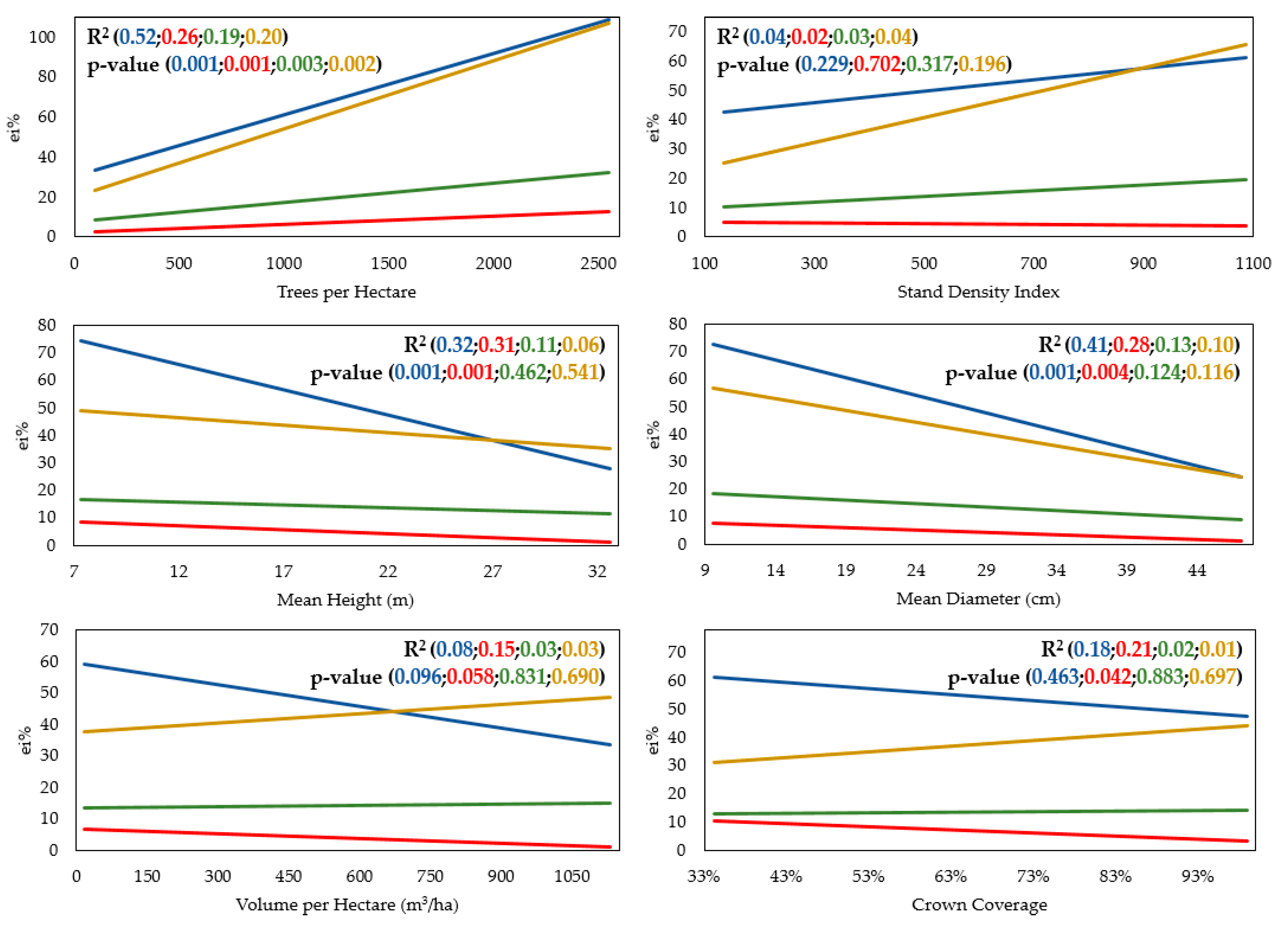
We then investigated the effect of selected stand parameters (i.e., trees per hectare, stand density index, mean height, mean diameter, crown coverage, volume per hectare) on the performance of remote-based inventory techniques used in this study (Figure 7).

None of the remotely-sensed attributes showed special sensitivity to selected stand parameters, but the accuracy of the used approach was found to be mostly related to the number of trees per hectare. In this case, the effect on all remotely-sensed attributes was significant. The significant effect was further confirmed between the parameters representing the mean basal area (quadratic mean height and diameter) and tree detection, as well as the remotely-sensed mean height. Significant effects were similarly observed between the crown coverage and remotely sensed mean height. Other parameters did not have a significant effect on the accuracy of the used approach (α = 0.05).

Regardless of statistical significance, the relationship between the forest structure and performance of the used approach was clear. The accuracy of tree detection decreased with increasing tree numbers per hectare and stand density index; however, this accuracy increased, as all other stand parameters increased. The accuracy of the remotely-sensed mean height decreased with increasing tree numbers per hectare, but increased as all other stand parameters increased. The accuracy of the remotely-sensed mean diameter, as well as the volume, decreased with increasing tree numbers per hectare, stand density index, volume per hectare, and crown coverage, as well as decreasing mean height and mean diameter.

Forest stands are defined as a group of trees occupying a specific area, and stand parameters, such as mean height, mean diameter, and growing stock, provide basal quantitative information about the structure of forest stands. In this sense, this information relates directly to silvicultural or environmental decisions and plays a key role in the management of natural resources. Unlike our proposed method, most studies related to the ITD-based approach have used a canopy height model as input for the extraction or derivation of stand characteristics. Point-based techniques are used less often, as these techniques often require time-consuming calculations. For example, using the same algorithm used in our study but based on lightweight aerial scanner data, Sačkov et al. [30] achieved accuracies over a multilayered broadleaved forest within ranges of 4–17%, 22–40%, and 40–45% for stand height, stand diameter, and growing stock, respectively. Woods et al. [51] provided similar results to our study using low-density ALS data over natural hardwoods and conifers and reported accuracies within ranges of 6–12%, 11–20%, and 22–23% for stand height, stand diameter, and growing stock, respectively.

4. Conclusions

The main objective of this study was to assess the usability and accuracy of an inventory for multistory mixed forests under close-to-nature management based on a combination of discrete airborne LiDAR data and multispectral aerial images using an individual tree-detection approach.

The results showed that this approach could be used for the remote-based estimation of various tree and stand inventory variables, including the number of trees, tree species, tree height, tree diameter, and tree volume. With respect to other studies, our findings indicated that airborne LiDAR data are suitable mainly for the detection of overstory trees and the estimation of the heights of those trees. The algorithm achieved less success regarding tree detection of understory trees, tree diameter derivation, and tree volume calculation. The main weakness of our proposed workflow was the aerial image-based classification of tree species composition. Although only groups of coniferous and broadleaved trees were classified, the obtained overall accuracy was insufficient. We argue, however, that the problem lies mainly in the quality of available images. Thus, the thorough preparation of flight missions and precise post-processing should ensure better results of tree species classification in the future. Multiple observations of the same area or the use of aerial or satellite images at different phenological stages would also definitely help separate coniferous and deciduous trees. Additionally, using true-ortophoto images or advanced methods for fusion of ALS data and ortophoto images, such as back-projecting [52], is a promising solution with a higher level of objectivity. Despite the shortcomings of this approach, the results were still positive at the stand level for practical use within forestry. There is the major benefit that the accuracy of the total growing stock calculated based on the remotely-sensed data was close to ±20% of the limit defined for the volume calculation in several European countries.

In this context, future research should be concerned with building more precise models for stem diameter derivation, and trying enhanced methods for the fusion of airborne laser scanning and imaging data. Subsequently, additional testing of our approach within a praxis of forest inventories under different ecosystems and data quality is needed.

References

1. Pukkala, T. Which type of forest management provides most ecosystem services? For. Ecosyst. 2016, 3, 9. [Google Scholar] [CrossRef]
2. Möller, A. Der Dauerwaldgedanke—Sein Sinn und Seine Bedeutung; Springer: Berlin, Germany, 1922; p. 136. [Google Scholar]
3. Bauhus, J.; Puettmann, K.J.; Kühne, C. Close-to-nature forest management in Europe: Does it support complexity and adaptability of forest ecosystems? In Managing Forests as Complex Adaptive Systems; Messier, C., Puettmann, K.J., Coates, K.D., Eds.; Routledge: London, UK; New York, NY, USA, 2014; pp. 187–213. [Google Scholar]
4. Gadow, K.; Nagel, J.; Saborowski, J. Continuous Cover Forestry. Managing Forest Ecosystems; Kluwer Academic Publishers: Dordrecht, The Netherlands, 2002; p. 348. [Google Scholar]
5. Eysn, L.; Hollaus, M.; Lindberg, E.; Berger, F.; Monnet, J.M.; Dalponte, M.; Kobal, M.; Pellegrini, M.; Lingua, E.; Mongus, D.; et al. A Benchmark of Lidar-Based Single Tree Detection Methods Using Heterogeneous Forest Data from the Alpine Space. Forests 2015, 6, 1721–1747. [Google Scholar] [CrossRef] [Green Version]
6. Kulla, L.; Sačkov, I.; Juriš, M. Test of airborne laser scanning ability to refine and streamline growing stock estimations by yield tables in different stand structures. For. J. 2016, 62, 39–47. [Google Scholar] [CrossRef]
7. Naesset, E. Estimating timber volume of forest stands using airborne laser scanner data. Remote Sens. Environ. 1997, 51, 246–253. [Google Scholar] [CrossRef]
8. Hyyppä, J.; Yu, X.; Hyyppä, H.; Hyyppä, M.; Holopainen, M.; Kukko, A.; Kaartinen, H.; Jaakkola, A.; Vaaja, M.; Koskinen, J.; et al. Advances in forest inventory using Airborne Laser Scanning. Remote Sens. 2007, 1190–1207. [Google Scholar] [CrossRef]
9. Hansen, E.H.; Ene, L.T.; Mauya, E.W.; Patočka, Z.; Mikita, T.; Gobakken, T.; Naesset, E. Comparing Empirical and Semi-Empirical Approaches to Forest Biomass Modelling in Different Biomes Using Airborne Laser Scanner Data. Forests 2017, 8, 170. [Google Scholar] [CrossRef]
10. Jaskierniak, D.; Kuczera, G.; Benyon, R.; Wallace, L. Using Tree Detection Algorithms to Predict Stand Sapwood Area, Basal Area and Stocking Density in Eucalyptus regnans Forest. Remote Sens. 2015, 7298–7323. [Google Scholar] [CrossRef]
11. Smreček, R.; Danihelová, Z. Forest stand height determination from low point density airborne laser scanning data in Rožňava Forest enterprise zone (Slovakia). iForest 2013, e1–e7. [Google Scholar] [CrossRef]
12. Zhen, Z.; Quackenbush, L.J.; Zhang, L. Trends in Automatic Individual Tree Crown Detection and Delineation—Evolution of LiDAR Data. Remote Sens. 2016, 8, 333. [Google Scholar] [CrossRef]
13. Ørka, H.O.; Dalponte, M.; Gobakken, T.; Næsset, E.; Ene, L.T. Characterizing forest species composition using multiple remote sensing data sources and inventory approaches. Scand. J. For. Resour. 2013, 28, 677–688. [Google Scholar] [CrossRef]
14. Packalén, P.; Maltamo, M. The k-MSN method in the prediction of species specific stand attributes using airborne laser scanning and aerial photographs. Remote Sens. Environ. 2007, 109, 328–341. [Google Scholar] [CrossRef]
15. Kandare, K.; Dalponte, M.; Ørka, H.O.; Frizzera, L.; Næsset, E. Prediction of Species-Specific Volume Using Different Inventory Approaches by Fusing Airborne Laser Scanning and Hyperspectral Data. Remote Sens. 2017, 9, 400. [Google Scholar] [CrossRef]
16. Breidenbach, J.; Næsset, E.; Lien, V.; Gobakken, T.; Solberg, S. Prediction of species specific forest inventory attributes using a nonparametric semi-individual tree crown approach based on fused airborne laser scanning and multispectral data. Remote Sens. Environ. 2010, 114, 911–924. [Google Scholar] [CrossRef]
17. Melville, G.; Stone, C.; Turner, R. Application of LiDAR data to maximise the efficiency of inventory plots in softwood plantations. N. Z. J. For. Sci. 2015, 45, 16. [Google Scholar] [CrossRef]
18. Flewelling, J.W. Probability models for individually segmented tree crown images in a sampling context. In Proceedings of the SilviLaser 2008 8th International Conference on LiDAR Applications in Forest Assessment and Inventory, Heriot-Watt University, Edinburgh, UK, 17–19 September 2008; pp. 284–294. [Google Scholar]
19. Kansanen, K.; Vauhkonen, J.; Lahivaara, T.; Mehtatalo, L. Stand density estimators based on individual tree detection and stochastic geometry. Can. J. For. Res. 2016, 46, 1359–1366. [Google Scholar] [CrossRef]
20. Lahivaara, T.; Seppanen, A.; Kaipio, J.P.; Vauhkonen, J.; Korhonen, L.; Tokola, T.; Maltamo, M. Bayesian approach to tree detection based on airborne laser scanning data. IEEE Trans. Geosci. Remote Sens. 2014, 52, 2690–2699. [Google Scholar] [CrossRef]
21. Chen, Y.; Zhu, X. An integrated GIS tool for automatic forest inventory estimates of Pinus radiata from LiDAR data. GISci. Remote Sens. 2013, 50, 667–689. [Google Scholar] [CrossRef]
22. Reitberger, J.; Schnörr, C.; Krzystek, P.; Stilla, U. 3D Segmentation of single trees exploiting full waveform LiDAR data. ISPRS J. Photogramm. Remote Sens. 2009, 64, 561–574. [Google Scholar] [CrossRef]
23. Wang, Y.; Weinacker, H.; Koch, B.; Sterenczak, K. Lidar point cloud based fully automatic 3D single tree modelling in forest and evaluations of the procedure. International Archives of Photogrammetry. Remote Sens. Spat. Inf. Sci. 2008, 37, 45–51. [Google Scholar]
24. Mongus, D.; Žalik, B. An efficient approach to 3D single tree-crown delineation in LiDAR data. ISPRS J. Photogramm. Remote Sens. 2015, 108, 219–233. [Google Scholar] [CrossRef]
25. Sačkov, I.; Hlásny, T.; Bucha, T.; Juriš, M. Integration of tree allometry rules to treetops detection and tree crowns delineation using airborne lidar data. iForest 2017, 10, 459–467. [Google Scholar] [CrossRef]
26. Kraus, K. Photogrammetry; Dummler Verlag: Bonn, Germany, 1993. [Google Scholar]
27. Petráš, R.; Pajtík, J. Sústava cesko-slovenských objemových tabuliek drevín. Lesnícky časopis 1991, 37, 49–56. (In Slovak) [Google Scholar]
28. Vauhkonen, J.; Ene, L.; Gupta, S.; Heinzel, J.; Holmgren, J.; Pitkänen, J.; Solberg, S.; Wang, Y.; Weinacker, H.; Hauglin, K.M.; et al. Comparative testing of single-tree detection algorithms under different types of forest. Forestry 2011, 85, 27–40. [Google Scholar] [CrossRef]
29. Kaartinen, H.; Hyyppä, J.; Yu, X.; Vastaranta, M.; Hyyppä, H.; Kukko, A.; Holopainen, M.; Heipke, C.; Hirschmugl, M.; Morsdorf, F.; et al. An International Comparison of Individual Tree Detection and Extraction Using Airborne Laser Scanning. Remote Sens. 2013, 4, 950–974. [Google Scholar] [CrossRef] [Green Version]
30. Sačkov, I.; Santopuoli, G.; Bucha, T.; Lasserre, B.; Marchetti, M. Forest Inventory Attribute Prediction Using Lightweight Aerial Scanner Data in a Selected Type of Multilayered Deciduous Forest. Forests 2016, 7, 307. [Google Scholar] [CrossRef]
31. Duncanson, L.; Cook, B.; Hurtt, G.; Dubayah, R. An efficient, multi-layered crown delineation algorithm for mapping individual tree structure across multiple ecosystems. Remote Sens. Environ. 2014, 154, 378–386. [Google Scholar] [CrossRef]
32. Ferraz, A.; Bretar, F.; Jacquemoud, S.; Gonçalves, G.; Pereira, L.; Tomé, M.; Soares, P. 3-D mapping of a multi-layered Mediterranean forest using ALS data. Remote Sens. Environ. 2012, 121, 210–223. [Google Scholar] [CrossRef]
33. Lu, X.; Guo, Q.; Li, W.; Flanagan, J. A bottom-up approach to segment individual deciduous trees using leaf-off lidar point cloud data. ISPRS J. Photogramm. Remote Sens. 2014, 94, 1–12. [Google Scholar] [CrossRef]
34. Solberg, S.; Næsset, E.; Bollandsås, O.M. Single-tree segmentation using airborne laser scanner data in a structurally heterogeneous spruce forest. Photogramm. Eng. Remote Sens. 2006, 72, 1369–1378. [Google Scholar] [CrossRef]
35. Sibona, E.; Vitali, A.; Meloni, F.; Caffo, L.; Dotta, A.; Lingua, E.; Motta, R.; Garbarino, M. Direct Measurement of Tree Height Provides Different Results on the Assessment of LiDAR Accuracy. Forests 2017, 8, 7. [Google Scholar] [CrossRef]
36. Brandtberg, T.; Warner, T.; Landenberger, R.; McGraw, J. Detection and analysis of individual leaf-off tree crowns in small-footprint, high sampling density LiDAR data from eastern deciduous forest in North America. Remote Sens. Environ. 2003, 85, 290–303. [Google Scholar] [CrossRef]
37. Gaveau, D.L.A.; Hill, R.A. Quantifying canopy height underestimation by laser pulse penetration in small-footprint airborne laser scanning data. Can. J. Remote Sens. 2003, 29, 650–657. [Google Scholar] [CrossRef]
38. Chávez, J.S.; Tullis, J.S. Deciduous Forest Structure Estimated with LiDAR-Optimized Spectral Remote Sensing. Remote Sens. 2013, 5, 155–182. [Google Scholar] [CrossRef]
39. Ballanti, L.; Blesius, L.; Hines, E.; Kruse, B. Tree Species Classification Using Hyperspectral Imagery: A Comparison of Two Classifiers. Remote Sens. 2016, 8, 445. [Google Scholar] [CrossRef]
40. Manzanera, J.A.; García-Abril, A.; Pascual, C.; Tejera, R.; Martín-Fernández, S.; Tokola, T.; Valbuena, R. Fusion of airborne LiDAR and multispectral sensors reveals synergic capabilities in forest structure characterization. GISci. Remote Sens. 2016, 53, 723–738. [Google Scholar] [CrossRef]
41. Sedliak, M.; Sačkov, I.; Kulla, L. Classifcation of tree species composition using a combination of multispectral imagery and airborne laser scanning data. Cent. Eur. For. J. 2017, 63, 1–9. [Google Scholar] [CrossRef]
42. Vaughn, N.R.; Moskal, L.M.; Turnblom, E.C. Tree Species Detection Accuracies Using Discrete Point Lidar and Airborne Waveform Lidar. Remote Sens. 2012, 4, 377–403. [Google Scholar] [CrossRef]
43. Prieditis, G.; Šmits, I.; Arhipova, I.; Dagis, S.; Dubrovskis, D. Tree Diameter Models from Field and Remote sensing data. Int. J. Math. Models Methods Appl. Sci. 2012, 6, 707–714. [Google Scholar]
44. Maltamo, M.; Gobakken, T. Predicting Tree Diametre Distributions. In Forestry Application of Airborne Laser Scanning: Concept and Case Studies; Maltamo, M., Næsset, E., Vauhkonen, J., Eds.; Springer: Dordrecht, The Netherlands, 2014; pp. 1–16. [Google Scholar]
45. Næsset, E. Practical large-scale forest stand inventory using a small-footprint airborne scanning laser. Scand. J. For. Resour. 2004, 19, 164–179. [Google Scholar] [CrossRef]
46. Tesfamichael, S.G.; Aardt, J.A.N.; Ahmed, F. Estimating plot-level tree height and volume of Eucalyptus grandis plantations using small-footprint, discrete return LiDAR data. Prog. Phys. Geogr. 2010, 34, 515–540. [Google Scholar] [CrossRef]
47. Means, J.E.; Acker, S.S.; Fitt, B.J.; Renslow, M.; Emerson, L.; Hendrix, C.J. Predicting forest stand characteristics with airborne scanning LiDAR. Photogramm. Eng. Remote Sens. 2000, 66, 1367–1371. [Google Scholar]
48. Andersen, H.E.; Strunk, J.; Temesgen, H.; Atwood, D.; Winterberger, K. Using multi-level remote sensing and ground data to estimate forest biomass resources in remote regions: A case study in the boreal forests of interior Alaska. Can. J. Remote Sens. 2011, 37, 596–611. [Google Scholar] [CrossRef]
49. Vauhkonen, J.; Mehtätalo, L.; Packalén, P. Combining tree height samples produced by airborne laser scanning and stand management records to estimate plot volume in Eucalyptus plantations. Can. J. Remote Sens. 2011, 41, 1649–1658. [Google Scholar] [CrossRef]
50. Hernandez-Marin, S.; Wallace, A.M.; Gibson, G.J. Bayesian Analysis of LiDAR Signals with Multiple Returns. IEEE Trans. Pattern Anal. Mach. Intell. 2007, 29, 2170–2180. [Google Scholar] [CrossRef] [PubMed]
51. Woods, M.; Lim, K.; Treitz, P. Predicting forest stand variables from LiDAR data in the Great Lakes—St. Lawrence forest of Ontario. For. Chron. 2008, 84, 827–839. [Google Scholar] [CrossRef]
52. Valbuena, R.; Mauro, F.; Arjonilla, F.J.; Manzanera, J.A. Comparing airborne laser scanning-imagery fusion methods based on geometric accuracy in forested areas. Remote Sens. Environ. 2011, 115, 1942–1954. [Google Scholar] [CrossRef]
Figure 1. Location of the study area: (a) normalized digital surface model; and (b) color-infrared aerial photograph.
Forests 08 00467 g001
Figure 2. Tree species composition on plots related to number of trees. C1-3, B1-3, M1-3: three development stages of coniferous, broadleaved, and mixed strata.
Forests 08 00467 g002
Figure 3. Detection rates of extracted (ER, blue histogram) and matched (MR, green histogram) individual trees for the strata. Commission rate (red line) is presented as well.
Forests 08 00467 g003
Figure 4. Regression between heights of field-measured trees (observed) and remotely-sensed trees (predicted) for coniferous strata (brown), broadleaved strata (green), and mixed strata (blue).
Forests 08 00467 g004
Figure 5. Regression between diameter of field-measured trees (observed) and remotely-sensed trees (predicted) for coniferous strata (brown), broadleaved strata (green), and mixed strata (blue).
Forests 08 00467 g005
Figure 6. Regression between volumes of field-measured trees (observed) and remotely-sensed trees (predicted) for coniferous strata (brown), broadleaved strata (green), and mixed strata (blue).
Forests 08 00467 g006
Figure 7. Regression between selected stand characteristics (X-axis) and relative individual difference (Y-axis) of remotely-sensed number of tree (blue), mean height (red), mean diameter (green), and volume (brown). The figures contain coefficients of determination (R2) and F-test of statistical significance of the regression model (p-value).
Forests 08 00467 g007