Mortality and Recovery of Hemlock Woolly Adelgid (Adelges tsugae) in Response to Winter Temperatures and Predictions for the Future

Abstract

Eastern (Tsuga canadensis) and Carolina hemlocks (T. caroliniana) of eastern North America have been attacked by the non-native hemlock woolly adelgid (Adelges tsugae Annand) (HWA) since the first half of the 20th century. Unlike most insects, HWA develops through one generation from fall to late winter, exposing this insect to the lethal effects of winter temperatures. The mortality inflicted by winter temperatures on HWA determines the surviving population density as well as its ability to spread to uninfested areas. With the ongoing changes in climate, knowledge of this species’ ability to survive and spread in the future can help land managers prepare for its management. This study began during the winter of 2014 and ended in the spring of 2017. During this period, winter mortality of HWA was recorded at 100 sites from Maine to Georgia (n = 209). Changes in population density from the sistens to the succeeding progrediens generation were recorded at 24 sites (n = 35). Models were developed to predict HWA mortality using the lowest minimum temperature prior to the mortality assessment date, the number of days with mean temperature <−1 °C, and the mean daily temperature of the three days preceding that minimum. Models were also developed to predict population density changes from the overwintering sistens generation to the following progrediens generation. Future projections under climate change showed increases in winter survival and population growth rates over time. Especially towards the northeastern edge of T. canadensis’ distribution as minimum temperatures are predicted to increase at a greater rate. This will result in an increase in density throughout its current distribution and expansion northward causing an increase in its impact on eastern Tsuga spp.

1. Introduction

Eastern hemlock (Tsuga canadensis (L.) Carrière) is distributed from the southeastern coastal areas of Canada, south through the Appalachian mountains to north Georgia, and west to eastern Ohio, Michigan, and Minnesota [1]. Throughout the Lake States, New England, and eastern Canada, this species is found at elevations up to 730 m. In the Mid-Atlantic States, it is found from 300 to 900 m, and in the southern Appalachians from 600 to 1525 m [2]. Carolina hemlocks (Tsuga caroliniana Engelm.) are found from south of the James River in Virginia to northern Georgia [3]. Eastern hemlocks prefer moist to very moist soils but can also tolerate drier soils and ridgetops [4]. Hemlocks are highly shade tolerant and occupy approximately 930,000 ha of hemlock dominated stands [5]. In the North, pure stands of hemlock create a species-poor understory while southern hemlocks grow in mixed stands of hardwoods in riparian zones along with dense thickets of rhododendron [6,7]. Eastern hemlock provides a unique habitat for numerous bird species in the northeastern United States that rely of this species for food, shelter, and reproduction [8]. The hemlock tree canopy shades the forest and moderates air and water temperatures resulting in warmer minimum and cooler maximum temperatures compared to an open exposed habitat [9]. This moderating effect on temperatures supports a unique suite of amphibians, fish, and invertebrates.

Hemlock woolly adelgid (HWA), Adelges tsugae Annand (Hemiptera: Adelgidae), was first recorded in the eastern U.S., infesting eastern hemlock in the early 1950s in Richmond, VA [10], but was likely present much earlier. HWA has caused significant health decline and death of eastern and Carolina hemlocks from Maine to Georgia [11,12,13,14] since its introduction from Japan [15]. Mortality of HWA infested hemlock can occur in four to 10 years, and entire hemlock stands can be killed by HWA [11,16,17].

Hemlock woolly adelgid has two asexual generations per year: sistens, and progrediens [18,19]. In Virginia, the sistens generation begins as eggs in late June [20]. The eggs hatch into first instar ‘crawlers’ that settle at the base of hemlock needles and remain there for the remainder of their lives. The first instar sistens immediately enter aestivation until mid-October when they begin developing. When the second instars appear, they secrete a wax-like flocculence covering their bodies that may provide a physical as well as a chemical defense [21]. They develop through four instars, beginning in late October in the mid-Atlantic states and reach the adult stage by early February. Sistens adults lay progrediens eggs from February through April. The progrediens eggs begin hatching into crawlers in early April, settle at the base of hemlock needles and develop through four instars to become adults in June and begin laying sistens eggs. The only stage that is capable of dispersing is the crawler stage before it inserts its stylet into the stem. Human movement and wildlife contribute to its dispersal [22], especially birds during spring migration [23]. HWA has been reported to spread at the rate of 15.6 km/year in the south, but more slowly (8.1 km/year) in the north, a reduction attributed to colder temperatures [24].

Trotter and Shields [25] cited several attributes for the rapid spread and high densities of HWA and their negative effects on T. canadensis and T. caroliniana. This species is bivoltine and parthenogenic with a sexual generation only on its primary spruce hosts (Picea species) [19]. However, its primary hosts are not suitable or available in the eastern U.S. where HWA reproduction is entirely asexual on its secondary Tsuga hosts. Because all HWA are female and sitesnes egg production ranges from 58 to 121 eggs/HWA [11,26], small populations can increase rapidly. In addition, no parasites have been reported in its native range or in the eastern U.S. [27,28] and no effective predators occur in the eastern U.S. [28]. Several predator species of HWA have been studied or released as biological control agents, primarily Laricobius nigrinus (Coleoptera: Derodontidae) and Sasajiscymnus tsugae (Coleoptera: Coccinelidae) in the eastern U.S. [29]. Finally, eastern Tsuga spp. appear to have little or no resistance or tolerance to feeding by HWA [30,31,32].

As with all insects, HWA is susceptible to many abiotic factors. During the summer aestivation period, high mortality has been reported due to exposure of excessive temperatures [33] and light [34,35]. HWA is unusual in that it actively feeds and develops during the winter, making it more vulnerable to extreme winter temperatures. The effect of minimum winter temperatures has received the most attention and is believed to be a barrier to northern expansion. A number of expressions of winter cold have been used to describe its effect on HWA: minimum winter temperature [25,36,37,38], number of days below subzero temperature thresholds [38,39], super cooling point [40,41], latitude [25,36], mean winter temperature [37], and a composite interactive-statistic using the sum of frequencies of subzero days multiplied by the respective minimum daily temperature [38]. Laboratory exposure to varying temperatures or cold-shock has also been conducted [42,43,44].

Paradis et al. [37] reported that when the mean winter temperature is equal to or above −5 °C, HWA mortality was below 91% and under these conditions, HWA will disperse to new areas. Based on a 15-year study of winter mortality of HWA in Connecticut, Cheah [38] reported that the absolute minimum temperature was the best predictor of mortality. Exposure to −24 to −21.2 °C resulted in 90% mortality of HWA and evidence of cold adaption in the colder regions of Connecticut was found. Tobin et al. [39] found a strong negative correlation between the number of days below subzero temperature thresholds and the HWA population growth rate during the extremely cold winter temperatures during the 2014 polar vortex. However, the detrimental effects were short lived and HWA densities rebounded by late summer to pre-2014 densities. Winter mortality has been reported to be over 90% at temperatures below −20 °C [25,37,38,42,43] and 100% mortality below −35 °C [44] and −40 °C [37]. The evidence for acclimatization or tolerance to cold has been contradictory, with reports of decline in cold hardiness after exposure to cold [42,45] and increases in cold hardiness as the winter progressed [38,41]. Differences in response to cold have also been found in winter survival between northern and southern HWA and these differences may be genetic [41,44,46]. These genetic differences have reportedly allowed HWA to reduce its cold mortality threshold northward and to have allowed expansion northward [46].

Low minimum temperatures obviously have a major impact on HWA survival with some evidence of regional differences in tolerance to cold [36,41,44]. Even at very low temperatures, a few HWA survive that may allow relatively quick recovery [47] and selection for more cold-tolerant populations [41,42]. Butin et al. [44] reported that even though they are parthenogenic, HWA populations are large enough for genetic mutations to occur that would allow adaptation to stochastic events such as extreme cold.

With an average warming of only ~1 °C, hundreds of studies have been published over the past decades that include observed and predicted impacts of climate change from the gene to ecosystem levels [48]. Several insect species have been documented to have expanded their range northward due to climate change. These include the Siberian silkmoth Dendrolimus sibiricus [49], the western spruce budworm Choristoneura occidentalis [50], the eastern spruce budworm C. fumiferana [51], and bark beetles [52]. The Colorado potato beetle Leptinotarsa decemlineata and its wild hosts (Solanum species) are expected to expand into both northern and southern regions [53] due to climate change. Recent warmer winters have reportedly affected the phenology of HWA by accelerating egg laying in western North Carolina [54]. An abiotic factor that has not received very much attention is photoperiod and the effect it may have on northward expanding species. Yee et al. [55] reported that detrimental effects of warming may occur for Aedes albopictus (Diptera: Culicidae) under longer photoperiods with northern range expansion resulting in lower fecundity.

Projections of climate change are difficult to predict and increase the uncertainty of predictions in insect–plant interactions [56,57,58]. However, developing models to predict range expansion and changes within its current range can help to better manage a pest and prepare for its potential invasion and increase in density. While multiple factors are involved in the dispersal, survival, development rate, and host interactions of insects, temperature is the main driver. With insects and the majority of their hosts being poikilotherms, they are critically dependent on temperature for their survival and development.

The genesis for this study occurred as a result of the occurrence of a polar vortex in January 2014 which was the second coldest winter in eastern North America since 1960 [59] followed by a second very cold winter in 2014/2015 caused by the Siberian express or Pacific–North American teleconnection pattern. This study was initiated to determine the effect of these severe cold events on HWA throughout its eastern distribution. Observations of HWA mortality were then recorded from southern Maine to northern Georgia during the winter of 2013–2014 and continued until the end of the 2017 winter. Assessments were also made on the density of the succeeding progrediens generation to determine to what degree HWA recovered. This is the first study on the effect of cold involving nearly the entire distribution of eastern HWA and the succeeding progrediens generation. With these data, a sub-continental scale predictive mortality model of HWA, based on winter temperatures and the subsequent change in density of the succeeding post-winter generation was developed and used to project changes in HWA survival in its current distribution and its future range expansion under a changing climate.

2. Materials and Methods

2.1. Winter Mortality

A protocol for assessing sistens mortality and progrediens recovery was sent to partners participating in the USDA Forest Service’s National HWA Initiative. This afforded a coordinated collection of data across the current distribution of HWAs from Maine to Georgia. Mortality of sistens was assessed from January to early April during the winters of 2014 to 2017. The mean number of HWA sistens examined per site was 510 and ranged from 19 to 2693. Hemlock woolly adelgid mortality was assessed at 100 sites during the four-year study, but not all of these sites were assessed each year. A single year will be used in this study to refer to a specific winter. For example, 2015 refers to the winter from 1 December 2014 to 28 February 2015. Each mortality assessment site was no more than 0.2 ha. Five to 15 infested branches (30–60 cm, length) with ample new growth were collected at each site from four to eight trees. Hemlock woolly adelgids found only on new growth were examined from the branches within 48 h after field collection. Hemlock woolly adelgid viability was assessed with a dissecting microscope.

To assess each individual as alive or dead, ethyl alcohol was dropped onto the HWA with forceps to dissolve the wax and make it easier to see the nymph. Hemlock woolly adelgids counted as killed during the winter were longer than 0.4 mm, but somewhat smaller than other live HWAs present at the time of assessment and when probed were dry and did not exude fluid. Hemlock woolly adelgids that had died within a week or so of assessment were similar in size to the largest HWAs but when gently probed, they exuded fluid from points other than where it was probed and had no leg or body movement. Live HWAs had full fresh wool, and when lightly probed did not exude fluid. The body retained its integrity when probed and expanded back to its original shape and legs also moved when probed. The adelgid was punctured only after firm probing and the hemolymph was fairly thick and dark red. The HWAs with these characteristics were counted as alive. The winter mortality rate was expressed as the number of dead HWAs divided by the total number alive and killed during the winter.

2.2. Progrediens Recovery

Assessments were made to determine the change in HWA density from the overwintering sistens generation to the progrediens generation after each winter from 2014–2017. These assessments were made at some but not all of the same locations at which mortality assessments were made. Sistens density assessment was conducted in February and March and the progrediens assessment was carried out in June. In February or March, a minimum of five trees were selected at each site. Twenty branches (30–40 cm long) with HWA were selected and flagged from the selected trees. The total number of HWAs from the point on the branch that was flagged to the terminal of each of the 20 flagged branches was counted in the field. No distinction was made between live or dead sistens; all sistens with wool were counted. Winter survival estimates were available for those sites from the winter mortality assessments described earlier. In June, the flagged branches examined during the sistens generation in February and March were examined for progrediens. All of the progrediens on these branches were counted. Since both live and dead sistens were counted for this assessment during the winter, the number of sistens that lived and survived the winter that would produce the progrediens generation was determined by multiplying the total number of sistens counted by the percent that survived based on the sistens mortality assessment made at that site. Laricobius nigrinus or S. tsugae are established at 19 of the 35 sites used for the progrediens recovery study, but the density in the early stages of their establishment may be low. The impact of these species whose larvae feed on the progrediens stage has been difficult to document [60]. Most HWA infestations will likely have one or both of these predators present in the future, so having them at these sites during this study will incorporate their effect in future infestations.

2.3. Temperature Data

The minimum and mean daily temperatures from 1 September to the date of sistens or progrediens assessment were generated using BioSIM [61]; ftp://ftp.cfl.scf.rncan.gc.ca/regniere/software/BioSIM/) at each site. BioSIM is a software product that simulates weather-driven processes at specific locations based on nearby weather station data, adjusting temperature with local gradients (latitude, longitude, elevation, and distance to shore). The daily weather database used was created from four sources of weather data: Environment Canada (http://climate.weather.gc.ca/index_e.html), GHCN-D (https://www.ncdc.noaa.gov/ghcn-daily-description), ISD-Lite (https://www.ncdc.noaa.gov/isd) and GSOD (https://data.noaa.gov/dataset/global-surface-summary-of-the-day-gsod) from 2013 to 2017. Daily minimum and mean air temperature were obtained with BioSIM at all sites and years from 1 September to the collection date of each sample for winter mortality and progrediens recovery assessments. Most of the sistens mortality samples were taken in late winter after the winter’s lowest temperatures had occurred. BioSIM can also generate an interpolated surface of model output across a geographic area from points, using Universal Kriging with elevation as an external drift variable. For mapping, 15,000 randomly distributed locations were generated across eastern North America with elevation extracted from the SRTM v4.1 digital elevation model at 3 arc-seconds horizontal resolution (http://www.cgiar-csi.org/data/srtm-90m-digital-elevation-database-v4-1). Cold mortality was simulated for each point and a surface was generated with a digital elevation model at 30 arc-seconds horizontal resolution.

2.4. Data Analysis

Models were developed to predict HWA mortality occurring from winter temperatures by determining for each sistens mortality observation the lowest minimum temperature of the winter (T_min) prior to the mortality assessment date. The number of days with mean temperature <−1 °C (N₋₁) prior to the date of occurrence of the extreme minimum were counted, to measure the potential cumulative effect of cold weather on survival. The mean temperature three days prior to the extreme minimum (Q₃) was also calculated, to test for cold acclimation. The choice of −1 °C and three days in the definitions of N₋₁ and Q₃ was arrived at by preliminary fitting of models with a simulated annealing algorithm to minimize the residual sum of squares between observations and predictions [62].

Models were also developed to predict population density changes from the overwintering sistens generation to the following progrediens generation. In all cases, T_min occurred prior to the sistens morality assessment, so this value did not change in the analysis of progrediens density assessments (t_p). For the prediction of progrediens density, additional variables used were the minimum temperature (T_min,pro) between sistens survival assessment (t_s) and progrediens density measurement (t_p), the number of cold days with a mean temperature <−1 °C (N_−1,pro), and the accumulation of degree days >0 °C (DD_pro) during the same period.

The sistens mortality rate (number dead per total number examined) were related to T_min, N₋₁, and Q₃ through binomial logistic regression [63] (SAS 9.4, PROC GENMOD, SAS Institute Inc., Cary, NC, USA). Four models were compared using the AIC (Akaike Information Criterion):

$$\ln \left(\frac{p}{1-p}\right)=p_0+p_1{T}_{\min }$$

(1)

$$\ln \left(\frac{p}{1-p}\right)=p_0+p_1{T}_{\min }+p_2{N}_{-1}+p_3{Q}_3$$

(2)

The third model used year as a class variable and T_min as a covariate:

$$\ln \left(\frac{p}{1-p}\right)=p_{0,y}+p_{1,y}{T}_{\min }$$

(3)

where p_0,y and p_1,y are year-specific intercepts and slopes. The fourth model used hardiness zone (5, 6, and 7) [64] as a class variable as a basis to compare the predictive ability of models based completely on weather data (Equations (1) and (2)):

$$\ln \left(\frac{p}{1-p}\right)=p_{0,Z}+p_{1,Z}{T}_{\min }$$

(4)

where p_0,Z and p_1,Z are hardiness zone-specific intercepts and slopes.

The growth of populations (r) from the sistens (S) to the progrediens generation (P), is defined as the ratio of the number of progrediens to live sistens (P/S) per sample, and it was analyzed with a General Linear Models procedure using the model:

$$\ln (r)=p_0+p_1\ln \left(S\right)+p_2{T}_{\min }+p_3{N}_{-1}+p_4{Q}_3+p_5{T}_{\min ,pro}+p_6{N}_{-1,pro}+p_{7}D{D}_{pro}$$

(5)

This model was then reduced by removing least-significant terms one at a time until all remaining terms were significant (α = 0.05).

2.5. Climate Change Projections

To predict current and future HWA mortality and population growth potential, minimum, and mean temperatures were generated for four periods at 30-year intervals (1981–2010, 2011–2040, 2041–2070, and 2071–2100). Future projections were computed for all weather stations in the BioSIM database by adjusting the 30-year normals for 1981–2010 by the delta method with the Canadian Regional Climate Model (CanRCM4 NAM22 RCP 4.5 driven by CCCma-CanESM2 (http://climate-modelling.canada.ca/climatemodeldata/canrcm/CanRCM4/index_cordex.shtml).

For each of the 15,000 simulation points used to construct maps, 101 years were simulated for each period by deaggregation of monthly normal to daily temperatures [65]. The temperature projections were also done at 26 locations along a southwest to northeast transect evenly spaced through the distribution of T. canadensis from 35° N, −84° E to 48° N, −66° E (Figure 1). The elevation of these 26 sites was obtained from the SRTM v4.1 digital elevation model. Sistens mortality and potential population growth resulting from the projected temperatures during each 30-year interval were generated using the best predictive model obtained above.

3. Results

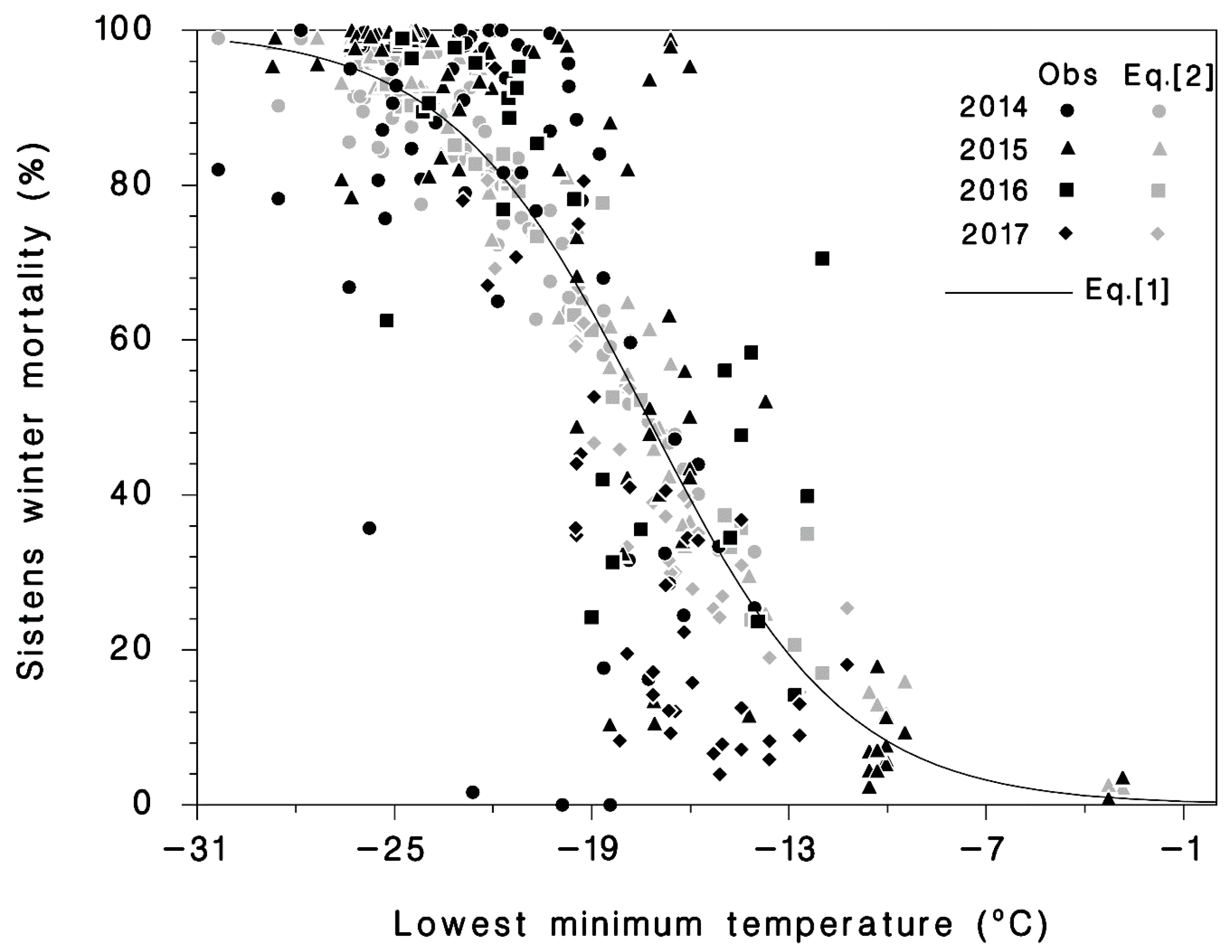
3.1. Winter Mortality

A total of 209 observations at 100 different sites of HWA sistens mortality during the winter were made from 2014 to 2017 from Maine to Georgia (Figure 1). The mean number of HWAs examined per site was 510 and ranged from 19 to 2693. The mean minimum temperature generated with BioSIM from 1 September until the date of the mortality assessment was −19.8 °C and ranged from −30.3 to −2.8 °C during the four-year study. The mean percent mortality was 65.3% and ranged from 0.8% to 100%. While it varied from site to site, the extreme minimum temperature experienced in 2014 was −30.3 at Mine Kill State Park, NY; −28.7, in 2015 near Fayetteville, WV; −25.2 in 2016 near Milford, MA; and −22.9 °C in 2017 near Erving, MA. The average extreme minimum temperatures among the 26 transect sites through the distribution of T. canadensis, were −24.1 ± 0.97, −24.4 ± 0.96, −21.3 ± 1.29, and −19.2 ± 1.01 °C in 2014, 2015, 2016, and 2017, respectively. Thus, 2017 was the warmest winter (Figure 2) and had the highest extreme minimum temperature, while 2014 and 2015 were the coldest.

The best model to predict sistens winter mortality based on the AIC (AIC = 22,554, the lower the value the better the fit) was year-specific Equation (3), with R² = 0.647 (

Table 1. Binomial logistic regression parameters (p’s) for winter mortality, Equations (1) to (4) where T_min is the lowest minimum temperature prior to the mortality assessment, N₋₁ is the number of days with mean temperature <−1 °C, and Q₃ is the mean temperature three days prior to the extreme minimum.

Equation	Coefficient	Standard Error	Wald χ2	p	AIC	R2
(1)					27,655	0.631
p0	−5.7290	0.0443	16,723	<0.0001
p1Tmin	−0.3311	0.0023	21,389	<0.0001
(2)					24,944	0.669
p0	−4.9946	0.0526	9,008	<0.0001
p1Tmin	−0.2760	0.0035	6,163	<0.0001
p2N−1	0.0549	0.0013	1,829	<0.0001
p3Q3	0.1416	0.0032	1,968	<0.0001
(3)					22,554	0.647
p0,2014	−2.3225	0.1760	1,089	<0.0001
p0,2015	−5.8618	0.1640	192	<0.0001
p0,2016	−4.8990	0.1887	293	<0.0001
p0,2017	−8.1307	0.1452	3,135	<0.0001
p1,2014 Tmin	−0.1767	0.0092	685	<0.0001
p1,2015 Tmin	−0.3666	0.0090	31	<0.0001
p1,2016 Tmin	−0.2975	0.0101	141	<0.0001
p1,2017 Tmin	−0.4168	0.0080	2,714	<0.0001
(4)					26,159	0.605
p0,5	−2.7359	0.2194	197	<0.0001
p0,6	−6.6776	0.1705	26	<0.0001
p0,7	−5.8135	0.1571	1,369	<0.0001
p1,5 Tmin	−0.1898	0.0115	169	<0.0001
p1,6 Tmin	−0.3852	0.0102	20	<0.0001
p1,7 Tmin	−0.3397	0.0096	1,262	<0.0001

). Equation (4), based on cold-hardiness zones (5, 6, and 7), had a higher AIC (26,159) and a lower R² = 0.605. For purposes of prediction, neither Equation (3) nor Equation (4) can be used as models because their parameter values apply either to specific years (2014–2017) or to specific cold-hardiness zones that will change under climate change. Therefore, the best predictive model, based on both AIC and R², was Equation (2) (Table 1; Figure 3) because it uses only weather data as input and can be used without alteration to predict sistens winter mortality under current and future climates. This model also provides evidence that accumulation of cold stress (N₋₁ term) increases winter mortality and that there is some cold acclimation in HWA, because the Q₃ term was also significant.

The simplest model, using only the minimum temperature (T_min) was Equation (1) with the highest AIC (27,655) and R² = 0.631 (Table 1, Figure 3). Equation (2) was intermediate, and with AIC = 24,944 and R² = 0.669, it was nearly as good as Equation (3) (Table 1; Figure 3). Because Equation (2) uses only weather data and is not year or hardiness zone specific, it can be used to predict sistens winter mortality under current and future climates. The analysis of Equation (2) provides evidence that accumulation of cold stress (N₋₁ term) increases winter mortality and that there is some cold acclimation in HWA, as the Q₃ term was also significant.

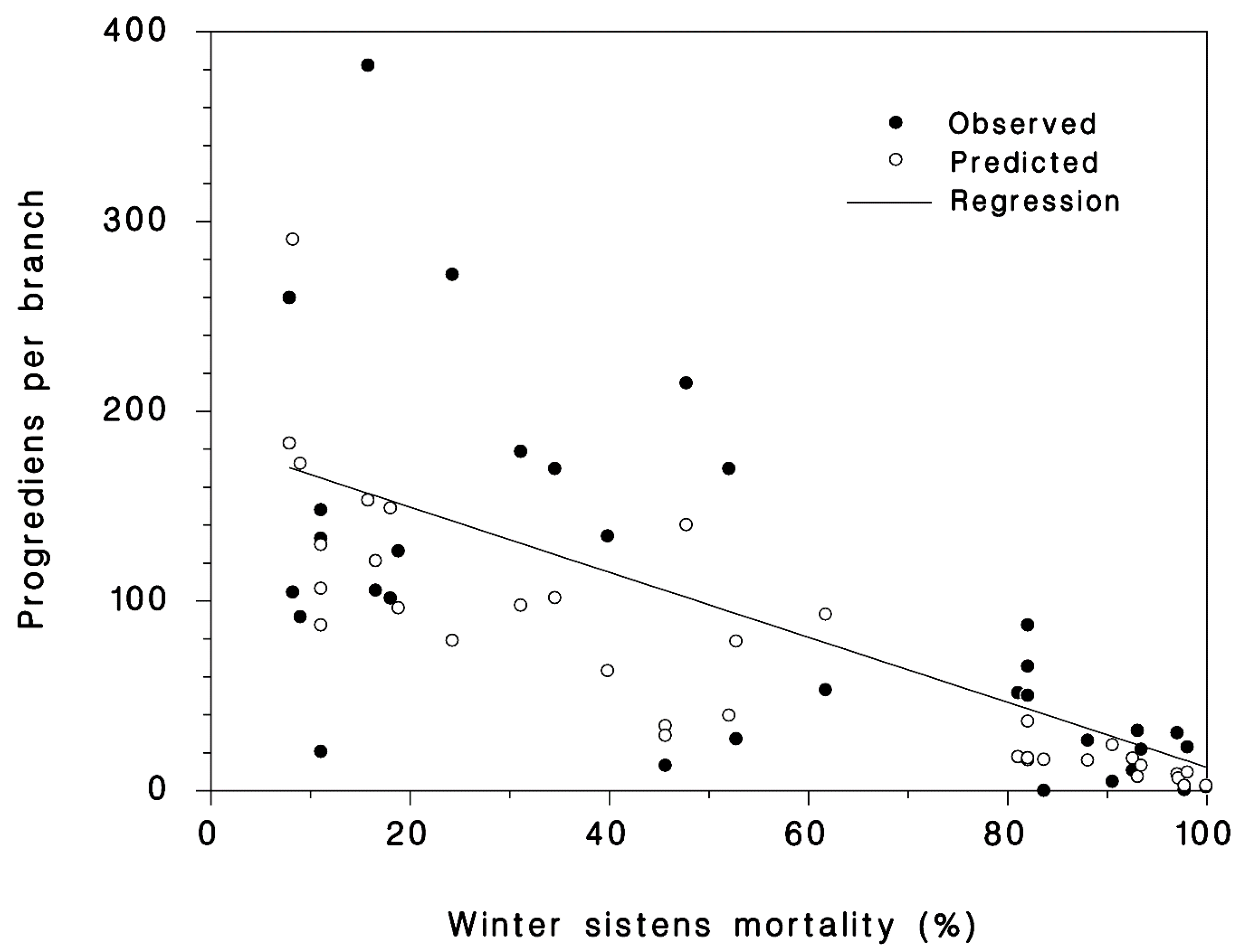
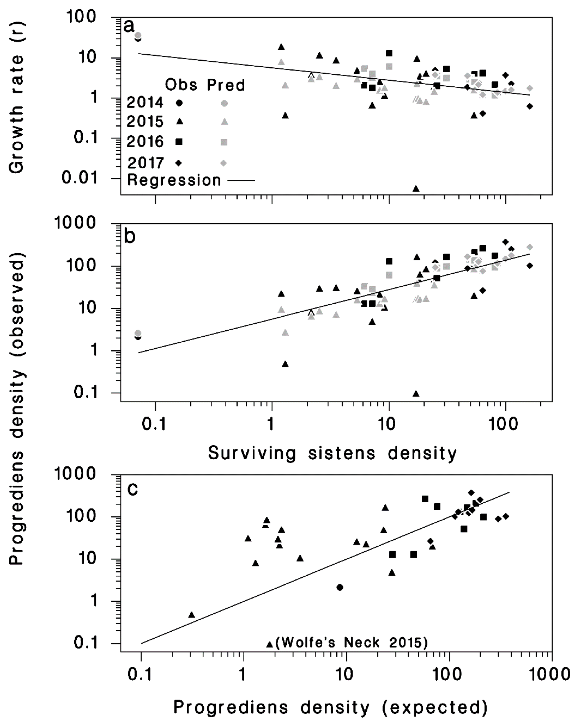
3.2. Progrediens Recovery

A total of 35 progrediens recovery observations were made from 24 sites by the US Forest Service’s National HWA Initiative collaborators in Massachusetts (5), Maryland (10), Maine (5), Ohio (6), Vermont (1), and Virginia (8) from 2014 to 2107. There was an overall observed mean of a 4.7-fold increase in density of the progrediens over the parental sistens generation that survived the winter. The lowest population growth rate from the sistens to the succeeding progrediens generation was 0.006 in Wolfe’s Neck, ME in 2015. Despite the very high mortalities of the sistens generation, the observed density of progrediens was greater than the live sistens density in 83% of the cases, with a mean observed increase of 4.7× and a maximum of 30.9×. The highest increase in progrediens occurred at Hussey Cr., VA, in 2014 that experienced a minimum temperature of −19.8 °C and had a predicted and observed sistens mortality of 70% and 99%, respectively. There was a significant (p < 0.001, R² = 0.71) negative relationship between winter mortality of sistens and the succeeding number of progrediens per branch (Figure 4). With a low sistens mortality of 10%, the predicted progrediens density was 144/branch. A 90% sistens mortality resulted in a predicted progrediens density of 12.6/branch.

The full model (Equation (5)) explained 33.6% of the variation in the rate of population growth (r) between live sistens and progrediens (

Table 2. Predictive binomial model parameters (p’s) for live sistens to progrediens (r = P/S) population change and statistics for Equations (5) and (6) where T_min is the lowest minimum temperature of the winter, N₋₁ is the number of days with mean temperature <−1 °C, Q₃ is the mean temperature three days prior to the extreme minimum, and S is the number of live sistens.

Equation	Coefficient	Standard Error	Student’s T	p	R2
(5)					0.336
p0	8.16900	2.71100	3.01	0.006
p1ln(S)	−0.65160	0.23190	−2.81	0.009
p2Tmin	0.23890	0.13790	1.73	0.095
p3N−1	0.01540	0.12110	0.13	0.899
p4Q3	0.00782	0.02736	0.29	0.777
p5Tmin,pro	0.04580	0.13540	0.34	0.738
p6N−1,pro	−0.05530	0.11900	−0.46	0.646
p7DDpro	−0.00131	0.00100	−1.30	0.203
(6)					0.251
p0	5.074	1.445	3.83	0.001
p1ln(S)	−0.5187	0.1651	−3.75	0.004
p2Tmin	0.14227	0.05831	3.09	0.020

). The number of cold days with a mean temperature <−1 °C (N₋₁ and N_−1pro), mean temperature three days prior to the extreme minimum (Q₃), and the accumulation of degree days >0 °C (DD_pro) were not significant and were not used in the final model. The reduced and final model, Equation (6), explained 25.1% of the variation, with the two significant terms, minimum temperature (T_min) and the number of live sistens (S) retained (Table 2, Figure 5a):

$$\ln (r)=\ln (P)-\ln (S)=p_0+p_1\ln \left(S\right)+p_2{T}_{\min }$$

(6)

These results suggest that the change in density from live sistens in the spring to the succeeding progrediens generation in the summer was negatively density-dependent, as indicated by the significance and negative sign of the ln(S) term in Equation (5) (Table 2). As the density of surviving sistens (S) increased, the rate of population growth to progrediens became smaller (Figure 5a). Live sistens densities of 50, 75, 100, and 125 would result in progrediens densities of 85, 113, 138, and 161 per branch, respectively, with population growth rates (r) of 1.7, 1.5, 1.4, and 1.3, respectively. Interestingly, the population growth rate (r) was positively related to the winter’s extreme minimum T_min, suggesting that some negative sublethal effect of extreme cold remained among surviving sistens. This sublethal cold effect may be a reduced fecundity resulting in lower progrediens density, but this hypothesis needs further investigation

Predicted progrediens density was obtained by rearranging Equation (6):

$$\widehat{P}=\exp \left[p_0+(1+p_1)\ln \left(S\right)+p_2{T}_{\min }\right]$$

(7)

The correlation between the density of surviving live sistens (S) and that of progrediens (P) was 0.629 (Figure 5b). There was no significant correlation between the density of progrediens and the total density of sistens (live and dead).

Progrediens density was predicted from the total density of sistens at the onset of winter by combining Equations (2) and (7):

$$\begin{array}{l}\widehat{S}=Z\left\{1-\frac{1}{1+\exp \left[-\left(-4.9946-0.276T_{\min }+0.0549N_{-1}+0.1416Q_3\right)\right]}\right\}\\ \widehat{P}=\exp \left[5.074+(1-0.5187)\ln \left(\widehat{S}\right)+0.14227T_{\min }\right]\end{array}$$

(8)

Progrediens density ($\widehat{P}$) predicted from total sistens density (Z) using Equation (8) was well correlated with observed progrediens density (R² = 0.68) (Figure 5c).

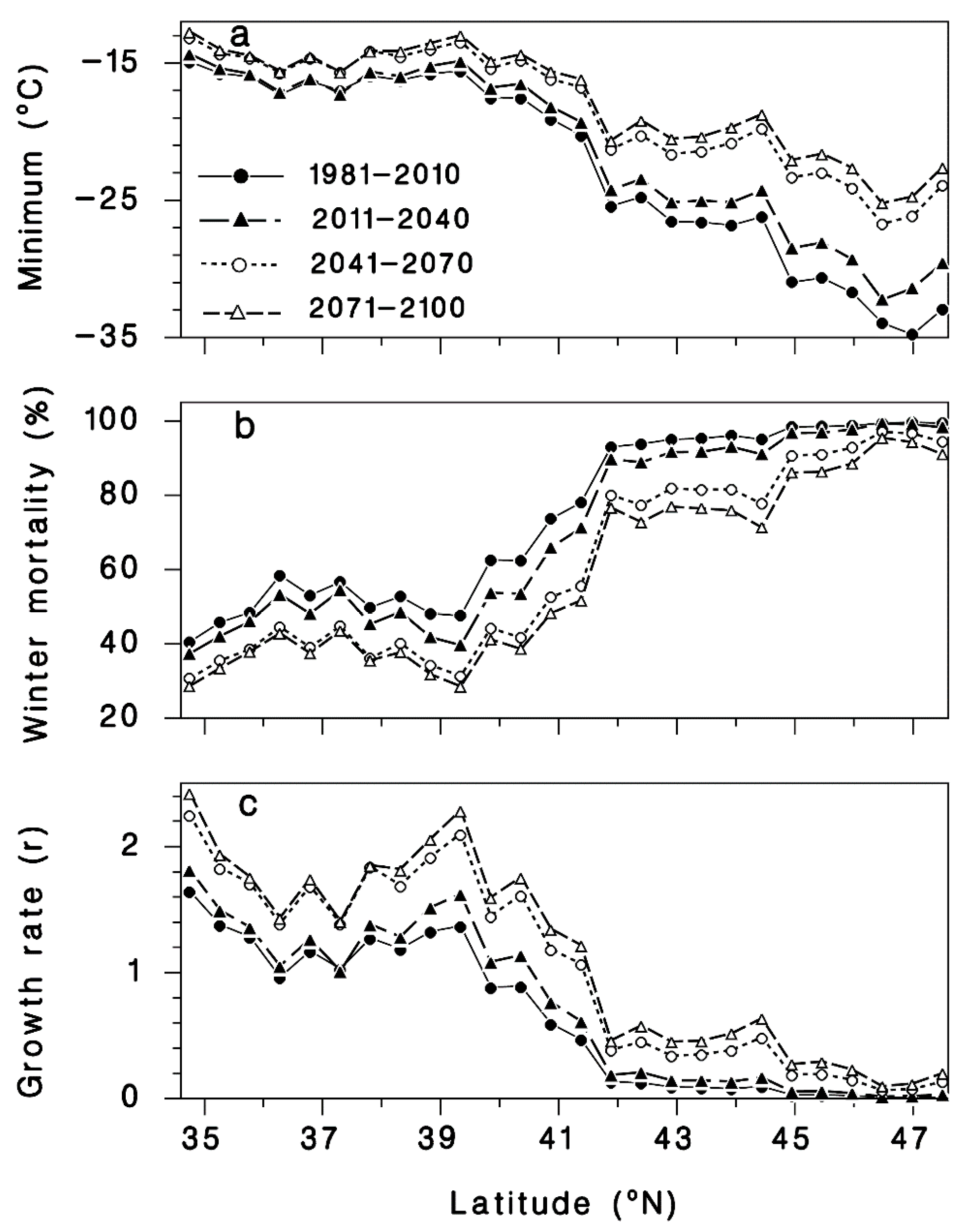
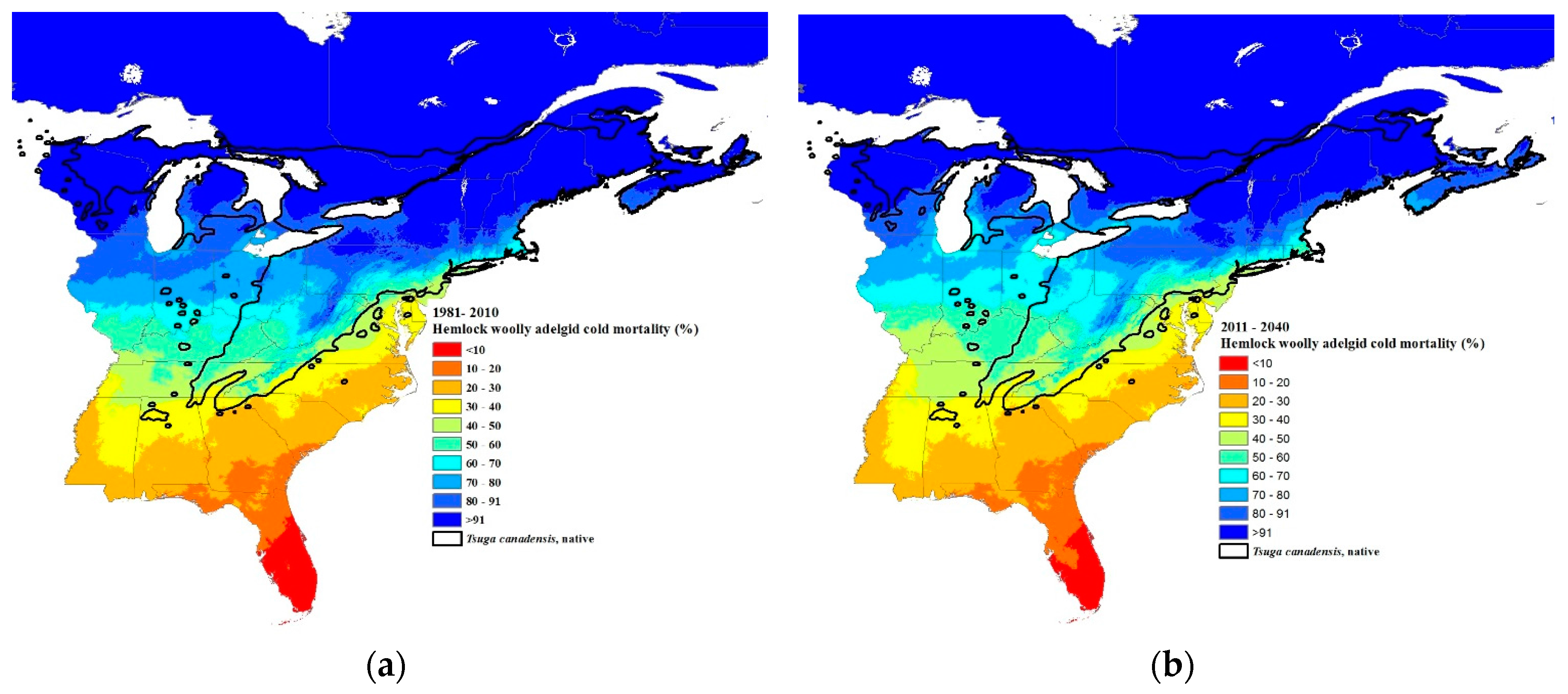
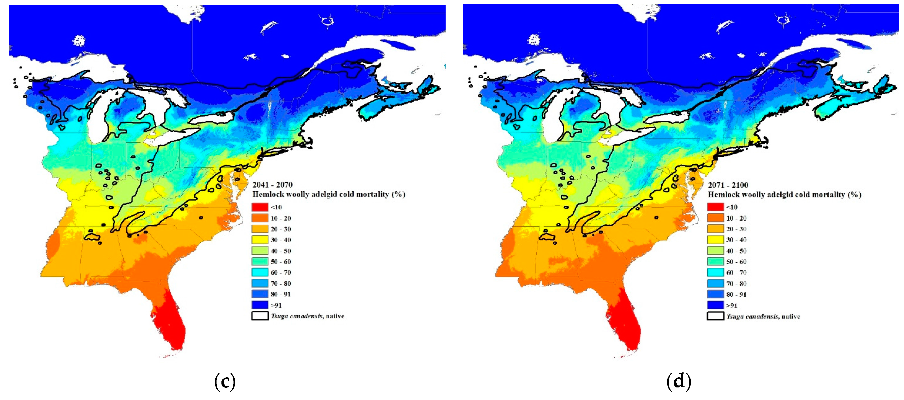
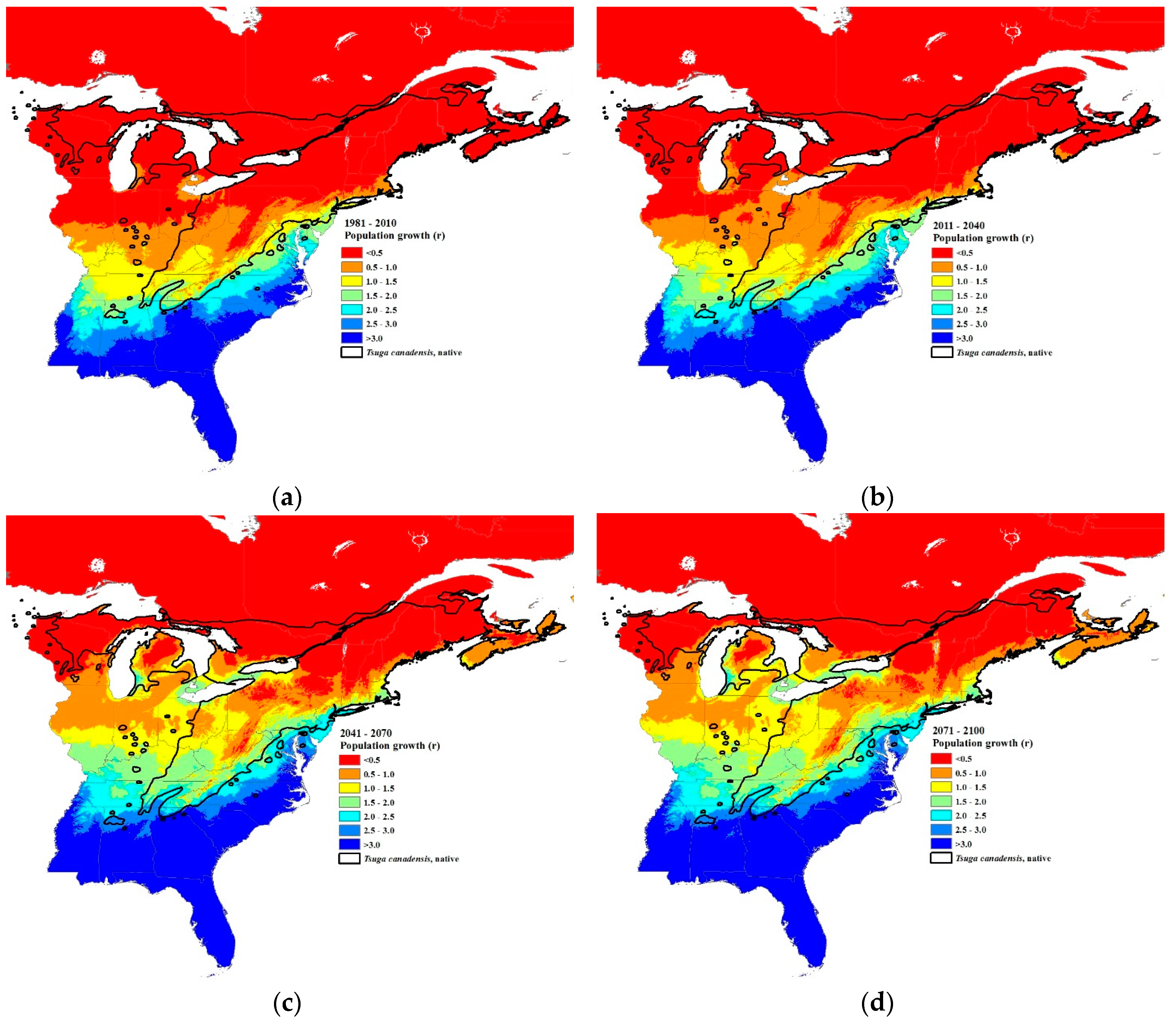
3.3. Climate Change Projections

The moderate (average) climate change scenario used in this study predicts a warming of extreme minimum winter temperatures, over the course of this century, that is more pronounced as latitude increases along the 26 transect sites through the current distribution of T. canadensis in eastern North America (Figure 6a). At the southernmost transect site (Figure 1), the mean minimum temperature is expected to rise from −14.9 °C based on the current 30-year normals (1981–2010) to −12.7 °C during the 2071–2100 interval, a 2.2 °C rise in minimum temperature (Figure 6a). At the northernmost site, the minimum temperature is expected to rise by more than 10.3 °C from −32.9 °C (current normals) to −22.6 °C by 2071–2100. Under this climate change scenario, Equation (2) predicts that HWA mortality should decrease, most notably in the northern part of eastern hemlock’s distribution (Figure 6b and Figure 7) in response to the pronounced rise in the minimum winter temperature.

The predicted winter mortality in the southernmost site (Figure 1) based on the current 30-year normals is 42% and is predicted to decrease to 30% by 2071–2100 (Figure 6b). The current most northern transect site where HWA is present is at the border of New Hampshire and Maine (Figure 1). The projected percent mortality at this location is predicted to decrease from 96% (based on current 30-year normals, 1981–2010) to 76% mortality by 2071–2100. While HWA is not yet present at the most northern transect site, if it were present based on the 30-year normals (1981–2010), percent mortality would be predicted to decrease from 99 to 91% at this northern site. HWA has recently been found in Michigan along the eastern shore of Lake Michigan [67]. HWA mortality in this area based on current 30-year normals (1981–2010) is projected to range from 70–80% (Figure 7a). By the 2071–2100, interval mortality is projected to decrease to 30–50% (Figure 7d), increasing the density of overwintering sistens. Projected mortalities are expected to decrease even lower in Nova Scotia due to the warming effects of the offshore currents. Mortalities for the 30-year normals (1981–2010) were predicted to be 80–100% (Figure 7a) while the 2071–2100-year interval mortalities were projected to be only 30–70% (Figure 7d), a 30–50% reduction in mortality.

Paradis et al. [37] estimated that mortality of 91% or less would result in the expansion of HWAs. Our estimates of where the 91% mortality isobar is for the current 30-year normals fit closely with the current distribution of HWAs, although in Vermont and New Hampshire, HWA has expanded north of the 91% mortality isobar (Figure 1 and Figure 7a). This suggests that a mortality rate of 91% or less is a good predictor of when HWA expansion can occur. Based on the HWA mortality threshold of 91%, HWA is projected to expand to all of Nova Scotia, central and northeastern Maine, all of New Hampshire, Vermont, New York (excluding the highest elevations), just north and south of the Saint Lawrence River in Quebec, southern Ontario, all of the lower Michigan peninsula, and all but the central upper peninsula, by the period 2071–2100.

Using Equation (8), applied to “average” HWA populations of 80 sistens per branch, HWA population growth rates should increase accordingly, throughout the host’s distribution (Figure 6c and Figure 8). The projected population growth rate (r = progrediens/sistens density) from the surviving sistens to the succeeding progrediens generation at the southernmost transect site (Figure 1), based on current 30-year normals (1981–2010), will increase 1.5-fold, from 1.6 to 2.4 by the 2071–2100 interval (Figure 6c and Figure 8). An even greater increase in recovery of the progrediens generation is predicted to occur at northern latitudes due to the greater increase in minimum temperature. At the current most northern HWA infested transect site at the Vermont–New Hampshire border, the progrediens generation has an r value of 0.08 based on current normals. However, by 2071–2100, the r value is projected to be 0.52, a 6-fold increase in recovery of the progrediens generation (Figure 6c and Figure 8). At the northern most transect site, if HWA were present currently, the r value is projected to be 0.013 based on the current normals. By 2071–2100, the r value is projected to be 0.204, a 16-fold increase. In the lower Michigan peninsula where HWA is currently found, the r value based on the current normals ranges from 0.5–1.0 (Figure 8a). By the 2011–2040-year interval, this is expected to increase to 1.5–2.5 (Figure 8d). In Nova Scotia, the r values for the 30-year normals (1981–2010) were predicted to be <1.0 (Figure 8a), while for the 2071–2100-year interval the r values were projected to increase to 0.5 to 2.0 (Figure 8d), a near doubling of the current HWA recovery rates in both regions. These r values in the northern range are less than 1.0, meaning that the succeeding progrediens generation would be less than the parent sistens generation. Yet due to parthenogenesis, this species can increase rapidly even at very low densities, suggesting that even at very low densities, HWA may be able to maintain their populations and even expand.

4. Discussion

Many studies have reported the negative effects of winter cold on the survival of HWAs [25,36,37,38,39,40,41,42,43,44,45]. This study incorporates the effect of winter cold mortality over a four-year period and a very broad geographic region, plus the resulting change in the sistens to progrediens population ratio to develop a model of winter survival and population growth. This model was used to predict changes in mortality and population density as climate change progresses during this century. Three indices were found to be useful in predicting future winter mortality: the extreme minimum temperature (T_min); the cumulative effect of cold, expressed as the number of days with a mean temperature <−1 °C (N₋₁); and to account for cold acclimation, the mean temperature of the three days prior to the extreme minimum (Q₃). Other studies have used other, often similar indices, but the one common index was extreme minimum winter temperature. Because of dissimilarities in indices used, our Equation (2) cannot be used to compare our observations with other reported mortality rates. However, Equation (1) (Figure 2) uses only minimum temperature, and does provide a basis for comparing the projections of mortality with other published models.

Differences in HWA winter mortality in climate divisions 1, 2, and 3 in a 15-year study were reported by Cheah [38] in Connecticut. The Connecticut climate divisions 1, 2, and 3 approximate hardiness zones 5b, 6a, and 6b, respectively. While several climate indices were used, such as the number of days below −17.8 °C and a composite interactive-statistic using the sum of frequencies of subzero days multiplied by the respective minimum daily temperature; the extreme minimum temperature was the most critical factor in predicting mortality using a non-linear sigmoid model. In the Connecticut climate division 1 (hardiness zone 5b), both our model and the Cheah [38] model predicted the same mortality of 90% at −24.0 °C. In climate division 2 (hardiness zone 6a) and climate division 3 (hardiness zone 6b), a 90% mortality was predicted by Cheah [38] at −22.4 and −21.2 °C, respectively. Our simple model predicted an 84% and 78% mortality at these temperatures, a 6% and 12% lower mortality, respectively. Our model predicted similar mortalities as those in climate divisions 1–3 at temperatures below −15 °C. Overall, mortalities in our study were somewhat higher for divisions 1 and 2 above −15 °C but quite similar to division 3 compared to the mortalities reported by Cheah [38].

Mortality assessments from 36 sites from Maine to Georgia were made during the winters of 2003 and 2004 to develop models to predict HWA mortality by Trotter and Shields [25]. The indices used in this study to predict mortality were latitude, altitude, minimum temperature, and HWA density. Altitude alone explained very little of the HWA survival and latitude about half. Only a weak link was found between HWA density and survival. Again, minimum temperature was the best indicator of mortality. Other studies have found no evidence of density-dependent survival of overwintering sistens [25,69]. Incorporating a density-dependent relationship in the winter mortality model would not have improved our model.

Differences in supercooling points and mortality response to winter temperatures have been found in HWA between hardiness zones and different climatic regions [41,43,45]. Lombardo and Elkinton [46] suggested that models developed for HWA winter survival should be unique to different geoclimatic regions. The inclusion of the two climatic descriptors in our Equation (2) model, the duration of the cold period, expressed as the number of days with mean temperature <−1 °C (N₋₁) and acclimation conditions, expressed as the mean temperature three days prior to the extreme minimum (Q₃), adequately expresses quantitatively what hardiness zones represent qualitatively. The cold hardiness model, Equation (4), also statistically did not provide as good a fit as Equation (2). Additionally, separate hardiness zone models would require the prediction of the changing distributions of zones over time under climate change incorporating more uncertainty and would become unwieldy to predict HWA winter mortality.

While previous models have used different indices to predict winter mortality, the simple model, Equation (1), using the minimum temperature only, developed in our study predicted mortalities similar to the mortalities predicted by others for temperatures below −18 °C. Above −18 °C, mortality projections varied considerably. Our simple model may be more conservative in predicting mortality, since it predicted higher mortalities than other models above −18 °C and consequently may predict a lower density of HWAs surviving the winter, resulting in a lower impact on hemlock trees. The full better fitting model, Equation (2), incorporates the number of days with mean temperature <−1 °C (N₋₁) prior to the date of occurrence of the extreme minimum, the mean temperature of the three days prior to the extreme minimum (Q₃), and the extreme minimum temperature and was an improvement over the simple model, Equation (1), which used only the minimum temperature. This improvement confirms the evidence from several studies that preconditioning or acclimatization does occur and this effect is incorporated in Equation (2). The acclimation to cold found by Elkinton [41] was similar in our study and incorporated in our model through the estimation of the unconstrained algorithm (simulated annealing) suggesting an acclimation (averaging) period of 3 days in determining Q₃. The combination of mortality predictions using the more complex model, Equation (2), with four years of mortality data across a broad landscape in addition to using the very robust climate prediction software resulted in a reliable projection model of future HWA winter mortality.

The change in density from the sistens to the succeeding progrediens generation varied considerably over the four-year study. Well over half of the sites exhibited an increase in the progrediens generation over the preceding sistens generation. While most of the progrediens populations were greater than the sistens, there was evidence of a negative density-dependent relationship of sistens to the succeeding progrediens: as the density of surviving sistens increased, the rate of progrediens density per branch decreased. This is a typical negative feedback of population density on population growth, likely caused by competition for resources as in the case of HWAs for optimal needle settling sites. McClure [11] and Sussky and Elkinton [69] found a similar negative density-dependent relationship.

Trotter and Shields [25] proposed that a survival rate of 2% of the overwintering sistens would result in a stable population and above 2% would allow an increase in population. Although their assumption of HWA survival, as related to minimum temperatures, was based on a linear relationship, our study found the relationship to be exponential. Paradis [37] postulated that a survival rate above 9% would result in expansion of HWAs, slightly greater than Trotter and Shields’ [25] rate of 2%. The Paradis [37] study was based on life table data and the HWA expansion rate of spread in Massachusetts. No data were presented for the recovery of HWAs from the sistens to the same succeeding progrediens population as was done in our study. Regardless of the high mortality that occurs during the winter, HWA populations have a tremendous capacity to increase. In our study, an overwintering mortality of 90% and 95% resulted in a density of 16 and 0.7 progrediens/branch, respectively. Tobin [47] reported that a single sistens adult with progrediens eggs can begin a new infestation on hemlock.

Other life stages of HWAs are also exposed to density-dependent and abiotic factors. Very high mortality rates from the settled first instar progrediens stage to the adult progrediens stage were reported by Sussky and Elkinton [68]. This high mortality was attributed to the very high fecundity rate of HWAs and the limited number of optimal feeding sites at the base of hemlock needles. Our study recorded the final density of adult progrediens but did not record the density of first instar progrediens. However, it could be assumed based on these studies that mortality during this stage would be high. Another mortality factor impacting HWA occurs during the summer due to high temperatures and possibly solar radiation. Higher HWA densities in low light conditions were found by Brantley [34], Sussky and Elkinton [69], Mayfield and Jetton [70], and Hickin and Preisser [71]. Mech [33] reported increased mortality of summer aestivating sistens with increases in temperature, particularly above 30 °C. McAvoy [35] reported that HWAs developing under shade had twice the survival rate compared to HWAs growing in full sun. Summer aestivating morality would be lower in the northern latitudes due to lower summer temperatures. Overwintering mortality, progrediens density-dependent mortality, and summer aestivating mortality all cause a large degree of HWA mortality; however, the preponderance of evidence indicates that overwintering mortality due to minimum winter temperatures is likely the major factor in determining its density and spread especially in the northern distribution of HWAs.

Based on our model to predict HWA mortality, survival, and progrediens recovery, it is clear that winter survival will increase along with an increase in population growth rates towards the northeastern edge of T. canadensis distribution. The effect of climate change on the host of HWAs, T. canadensis, should also be considered. Prasad and Potter [72] reported that future eastern hemlock habitats will decline and colonization beyond its current distribution will be very limited due to increases in aridity and temperature, while Dunckel [73] found that eastern hemlock will increase in range within Maine in a northwest expansion. Eastern hemlock may alter its distribution, but is unlikely to expand farther north of its current range. Higher temperatures will likely degrade hemlock habitat, reducing tree vigor, and making it more susceptible to feeding by HWA, compounded by the anticipated increase of HWA.

5. Conclusions

While the confidence levels of projecting temperature regimes into the future decrease as the years into the future increase, it is clear from this study that HWA winter mortality will decrease northward over the future decades. Correspondingly, HWA population growth rates should also increase northward over the years. Increasing the risk of HWA infestations manifesting themselves at ever higher latitudes within the range of the insect’s host tree. Based on these models, HWA may nearly reach the northern extent of eastern hemlock distribution. Only the most northern stands of hemlock and those at the higher elevations in its northern distribution may escape HWA. Even in its current distribution, HWA winter survival will increase, increasing its density and impact on eastern Tsuga spp. Management of HWA in its current range needs to continue with chemical and biological control efforts, especially in the northern range of HWA.

References

1. Godman, R.M.; Lancaster, K. Tsuga canadensis (L.) Carriere. In Silvics of North America: Conifers; Agriculture Handbook 654; Burns, R.M., Honkala, B.H., Eds.; USDA Forest Service: Washington, DC, USA, 1990; Volume 1, pp. 605–612. [Google Scholar]
2. Fowells, H.A. Silvics of Forest Trees of the United States; Agriculture Handbook No. 271; U.S. Department of Agriculture: Washington, DC, USA, 1965; 760p.
3. Jetton, R.M.; Dvorak, W.S.; Whittier, W.A. Ecological and genetic factors that define the natural distribution of Carolina hemlock in the Southeastern United States and their role in ex situ conservation. For. Ecol. Manag. 2008, 255, 3212–3221. [Google Scholar] [CrossRef]
4. Kessell, S.R. Adaption and dimorphism in eastern hemlock, Tsuga canadensis (L.) Carr. Am. Nat. 1979, 113, 333–350. [Google Scholar] [CrossRef]
5. McWilliams, W.H.; Schmidt, T.L. Composition, structure, and sustainability of hemlock ecosystems in Eastern North America. In Proceedings of the Symposium on Sustainable Management of Hemlock Ecosystems in Eastern North America, Durham, NH, USA, 22–24 June 1999; McManus, K.A., Shields, K.S., Souto, D.R., Eds.; USDA Forest Service: Washington, DC, USA, 1999. [Google Scholar]
6. Ellison, A.M.; Bank, M.S.; Clinton, B.D.; Colburn, E.A.; Elliott, K.; Ford, C.R.; Foster, D.R.; Kloeppel, B.D.; Knoepp, J.D.; Lovett, G.M.; et al. Loss of foundation species: Consequences for the structure and dynamics of forested ecosystems. Front. Ecol. Environ. 2005, 3, 479–486. [Google Scholar] [CrossRef]
7. Narayanaraj, P.V.; Bolstad, P.V.; Elliott, K.J.; Vose, J.M. Terrain and Landforms Influence on Tsuga canadensis (L.) Carrière (Eastern Hemlock) Distribution in the Southern Appalachian Mountains. Castanea 2010, 75, 1–8. [Google Scholar] [CrossRef]
8. Tingley, M.W.; Orwig, D.A.; Field, R.; Motzkin, G. Avian response to removal of a forest dominant: Consequences of hemlock woolly adelgid infestations. J. Biogeogr. 2002, 29, 1505–1516. [Google Scholar] [CrossRef]
9. Snyder, C.D.; Young, J.A.; Lemarié, D.P.; Smith, D.R. Influence of eastern hemlock (Tsuga canadensis) forests on aquatic invertebrate assemblages in headwater streams. Can. J. Fish. Aquat. Sci. 2002, 59, 262–275. [Google Scholar] [CrossRef]
10. Souto, D.; Luther, T.; Chianese, B. Past and current status of HWA in eastern and Carolina hemlock stands. In Proceedings of the First Hemlock Woolly Adelgid Review, Charlottesville, VA, USA, 12 October 1995; Salom, S.M., Tigner, T.C., Reardon, R.C., Eds.; USDA Forest Service: Morgantown, WV, USA, 1996; pp. 9–15. [Google Scholar]
11. McClure, M.S. Density-dependent feedback and population cycles in Adelges tsugae (Homoptera: Adelgidae) on Tsuga canadensis. Environ. Entomol. 1991, 20, 258–264. [Google Scholar] [CrossRef]
12. Orwig, D.A.; Foster, D.R. Forest response to the introduced hemlock woolly adelgid in southern New England. J. Torrey Bot. Soc. 1998, 125, 60–73. [Google Scholar] [CrossRef]
13. Morin, R.S.; Oswalt, S.N.; Trotter, R.T., III; Liebhold, A.W. Status of Hemlock in the Eastern United States Forest Inventory and Analysis Factsheet; e-Science Update SRS-038; U.S. Department of Agriculture Forest Service, Southern Research Station: Asheville, NC, USA, 2011; p. 4.
14. Orwig, D.A.; Thompson, J.R.; Povak, N.A.; Manner, M.; Niebyl, D.; Foster, D.R. A foundation tree at the precipice: Tsuga canadensis health after the arrival of Adelges tsugae in central New England. Ecosphere 2012, 3, 1–16. [Google Scholar] [CrossRef]
15. Havill, N.P.; Montgomery, M.E.; Yu, G.; Shiyake, S.; Caccone, A. Mitochondrial DNA from hemlock woolly adelgid (Hemiptera: Adelgidae) suggest cryptic speciation and pinpoints the source of the introduction to Eastern North America. Ann. Entomol. Soc. Am. 2006, 9, 195–203. [Google Scholar] [CrossRef]
16. Orwig, D.A.; Foster, D.R.; Mausel, D.L. Landscape patterns of hemlock decline in New England due to introduced hemlock woolly adelgid. J. Biogeogr. 2002, 29, 1475–1487. [Google Scholar] [CrossRef]
17. Eschtruth, A.; Cleavitt, N.L.; Battles, J.J.; Evans, R.A.; Fahey, T.J. Vegetation dynamics in declining eastern hemlock stands: 9 years of forest response to hemlock woolly adelgid infestation. Can. J. For. Res. 2006, 36, 1435–1450. [Google Scholar] [CrossRef]
18. McClure, M.S. Biology of Adelges tsugae and its potential for spread in the Northeastern United States. In Proceedings of the First Hemlock Woolly Adelgid Review, Charlottesville, VA, USA, 12 October 1995; FHTET 96-10. Salom, S.M., Tigner, T.C., Reardon, R.C., Eds.; USDA Service Center: Morgantown, WV, USA, 1996; pp. 16–25. [Google Scholar]
19. Havill, N.P.; Foottit, R.G. Biology and evolution of Adelgidae. Annu. Rev. Entomol. 2007, 52, 325–349. [Google Scholar] [CrossRef] [PubMed]
20. Gray, D.R.; Salom, S.M. Biology of hemlock woolly adelgid in the southern Appalachians. In Proceedings of the First Hemlock Woolly Adelgid Review, Charlottesville, VA, USA, 12 October 1995; Salom, S.M., Tigner, T.C., Reardon, R.C., Eds.; USDA Forest Service: Morgantown, WV, USA, 1996; pp. 26–35. [Google Scholar]
21. Jones, A.C.; Mullins, D.E.; Jones, T.H.; Salom, S.M. Potential feeding deterrents found in hemlock woolly adelgid, Adelges tsugae. Naturwissenschaften 2012, 99, 583–586. [Google Scholar] [CrossRef] [PubMed]
22. McClure, M.S. Role of wind, birds, deer, and humans in the dispersal of hemlock woolly adelgid (Homoptera: Adelgidae). Environ. Entomol. 1990, 19, 36–43. [Google Scholar] [CrossRef]
23. Russo, N.J.; Cheah, C.A.S.-J.; Tingley, M.W. Experimental evidence for branch-to-bird transfer as a mechanism for avian dispersal of the hemlock woolly adelgid (Hemiptera: Adelgidae). Environ. Entomol. 2016, 45, 1107–1114. [Google Scholar] [CrossRef] [PubMed]
24. Evans, A.M.; Gregoire, T.G. A geographical variable model of hemlock woolly adelgid spread. Biol. Invasions 2007, 9, 369–382. [Google Scholar] [CrossRef]
25. Trotter, R.T., III; Shields, K.S. Variation in winter survival of the invasive hemlock woolly adelgid (Hemiptera: Adelgidae) across the Eastern United States. Environ. Entomol. 2009, 38, 577–587. [Google Scholar] [CrossRef] [PubMed]
26. Jones, A.C.; Mullins, D.E.; Brewster, C.; Rhea, J.P.; Salom, S.M. Fitness and physiology of Adelges tsugae (Hemiptera: Adelgidae) in relation to the health of the eastern hemlock. Insect Sci. 2016, 23, 843–853. [Google Scholar] [CrossRef] [PubMed]
27. Montgomery, M.E.; Lyon, S.M. Natural enemies of adelgids in North America: Their prospect for biological control of Adelges tsugae (Homoptera: Adelgidae). In Proceedings of the First Hemlock Woolly Adelgid Review, Charlottesville, VA, USA, 12 October 1995; Salom, S.M., Tigner, T.C., Reardon, R.C., Eds.; USDA Forest Service: Morgantown, WV, USA, 1996; pp. 89–102. [Google Scholar]
28. Wallace, M.S.; Hain, F.P. Field surveys and evaluation of native and established predators of the hemlock woolly adelgid (Homoptera: Adelgidae) in the Southeastern United States. Environ. Entomol. 2000, 29, 638–644. [Google Scholar] [CrossRef]
29. Onken, B.P.; Reardon, R.C.; Technical Coordinators. Implementation and Status of Biological Control of the Hemlock Woolly Adelgid; Publication FHTET-2011-04; USDA Forest Service, Forest Health Technology Enterprise Team: Morgantown, WV, USA, 2011; p. 230.
30. Lagalante, A.F.; Lewis, N.; Montgomery, M.E.; Shields, K.S. Temporal and spatial variation in eastern hemlock (Tsuga canadensis) in relation to feeding by Adelges tsugae. J. Chem. Ecol. 2006, 32, 2389–2403. [Google Scholar] [CrossRef] [PubMed]
31. Bentz, S.E.; Montgomery, M.E.; Olsen, R.T. Resistance of hemlock species and hybrids to hemlock woolly adelgid. In Proceedings of the Fourth Symposium on Hemlock Woolly Adelgid in the Eastern United States, Hartford, CN, USA, 12–14 Feburary 2008; FHTET-2008-01. Onken, B., Reardon, R.C., Eds.; USDA Forest Service: Morgantown, WV, USA, 2008; pp. 137–139. [Google Scholar]
32. Ayayee, P.; Yang, F.; Rieske, L.K. Biomechanical properties of hemlocks: A novel approach to evaluating physical barriers of the plant-insect interface and resistance to a phloem-feeding herbivore. Insects 2014, 5, 364–376. [Google Scholar] [CrossRef] [PubMed]
33. Mech, A.M.; Tobin, P.C.; Teskey, R.O.; Rhea, J.R.; Gandhi, K.J.K. Increases in summer temperatures decrease the survival of an invasive forest insect. Bio. Invasions 2017. [Google Scholar] [CrossRef]
34. Brantley, T.S.; Mayfield, A.E., III; Jetton, R.M.; Miniat, C.F.; Zielow, D.R.; Brown, C.L.; Rhea, J.R. Elevated light levels reduce hemlock woolly adelgid infestation and improve carbon balance of infested eastern hemlock seedlings. For. Ecol. Manag. 2017, 385, 150–160. [Google Scholar] [CrossRef]
35. McAvoy, T.J.; Mays, R.; Johnson, N.G.; Salom, S.M. The effects of shade, fertilizer, and pruning on eastern hemlock trees and hemlock woolly adelgid. Forests 2017, 8, 156. [Google Scholar] [CrossRef]
36. Shields, K.S.; Cheah, A.S.-J. Winter mortality in Adelges tsugae populations in 2003 and 2004. In Proceedings of the Third Symposium on Hemlock Woolly Adelgid in the Eastern United States, Asheville, NC, USA, 1–3 Feburary 2005; Onken, B., Reardon, R., Eds.; USDA Forest Service: Morgantown, WV, USA, 2005; pp. 354–356. [Google Scholar]
37. Paradis, A.; Elkinton, J.; Hayhoe, K.; Buonaccorsi, J. Role of winter temperature and climate change on the survival and future range expansion of the hemlock woolly adelgid (Adelges tsugae) in Eastern North America. Mitig. Adapt. Strat. Glob. Chang. 2008, 13, 541–554. [Google Scholar] [CrossRef]
38. Cheah, C.A.S.-J. Predicting hemlock woolly adelgid winter mortality in Connecticut forests by climate divisions. Northeast. Nat. 2017, 24, B90–B118. [Google Scholar] [CrossRef]
39. Tobin, P.C.; Turcotte, R.M.; Blackburn, L.M.; Juracko, J.A.; Simpson, B.T. The big chill: Quantifying the effect of the 2014 North American cold wave on hemlock woolly adelgid populations in the central Appalachian Mountains. Popul. Ecol. 2017, 59, 251–258. [Google Scholar] [CrossRef]
40. Costa, S.D.; Trotter, R.T.; Montgomery, M.; Fortney, M. Low temperature in the hemlock woolly adelgid system. In Proceedings of the Fourth Symposium on Hemlock Woolly Adelgid in the Eastern United States, Hartford, CN, USA, 12–14 Feburary 2008; FHTET-2008-01. Onken, B., Reardon, R.C., Eds.; USDA Forest Service: Morgantown, WV, USA, 2008; pp. 47–52. [Google Scholar]
41. Elkinton, J.S.; Lombardo, J.A.; Roehrig, A.D.; McAvoy, T.J.; Mayfield, A.; Whitmore, M. Induction of cold hardiness in an invasive herbivore: The case of hemlock woolly adelgid (Hemiptera: Adelgidae). Environ. Entomol. 2017, 46, 118–124. [Google Scholar] [CrossRef] [PubMed]
42. Parker, B.L.; Skinner, M.; Gouli, S.; Ashikaga, T.; Teillon, H.B. Survival of hemlock woolly adelgid (Homoptera: Adelgidae) at low temperatures. For. Sci. 1998, 44, 414–420. [Google Scholar]
43. Parker, B.L.; Skinner, M.; Gouli, S.; Ashikaga, T.; Teillon, H.B. Low lethal temperature for hemlock woolly adelgid (Homoptera: Adelgidae). Environ. Entomol. 1999, 28, 1085–1091. [Google Scholar] [CrossRef]
44. Butin, E.; Porter, A.H.; Elkinton, J. Adaption during biological invasions and the case of Adelges tsugae. Evol. Ecol. Res. 2005, 7, 887–900. [Google Scholar]
45. Skinner, M.; Parker, B.L.; Gouli, S.; Ashikaga, T. Regional responses of hemlock woolly adelgid (Homoptera: Adelgidae) to low temperatures. Environ. Entomol. 2003, 32, 523–528. [Google Scholar] [CrossRef]
46. Lombardo, J.A.; Elkinton, J.S. Environmental adaption in an asexual invasive insect. Ecol. Evol. 2017. [Google Scholar] [CrossRef] [PubMed]
47. Tobin, P.C.; Turcotte, R.M.; Snider, D.A. When one is not necessarily a lonely number: Initial colonization dynamics of Adelges tsugae on eastern hemlock, Tsuga canadensis. Biol. Invasions 2013, 15, 1925–1932. [Google Scholar] [CrossRef]
48. Scheffers, B.R.; De Meester, L.; Bridge, T.C.L.; Hoffmann, A.A.; Pandolfi, J.M.; Corlett, R.T.; Butchart, S.H.M.; Pearce-Kelly, P.; Kovacs, K.M.; Dudgeon, D.; et al. The broad footprint of climate change from genes to biomes to people. Science 2016, 354. [Google Scholar] [CrossRef] [PubMed]
49. Kharuk, V.L.; Im, S.T.; Ranson, K.J.; Yagunov, M.N. Climate-Induced Northerly Expansion of Siberian Silkmoth Range. Forests 2017. [Google Scholar] [CrossRef]
50. Thomson, A.J.; Benton, R. A 90-year sea warming trend explains outbreak patterns of western spruce budworm on Vancouver Island. For. Chron. 2007, 83, 867–869. [Google Scholar] [CrossRef]
51. Régnière, J.; St.-Amant, R.; Duval, P. Predicting insect distributions under climate change from physiological responses: Spruce budworm as an example. Biol. Invasions 2012, 14, 1571–1586. [Google Scholar] [CrossRef]
52. Bentz, B.; Régnière, J.; Fettig, C.J.; Hansen, E.M.; Hayes, J.L.; Hicke, J.A.; Kelsey, R.G.; Lundquist, J.; Negrón, J.F.; Seybold, S.J. Climate change and bark beetles of the Western US and Canada: Direct and indirect effects. Bioscience 2010, 60, 602–613. [Google Scholar] [CrossRef]
53. Wang, C.; Hawthorne, D.; Qin, Y.; Pan, X.; Li, Z.; Zhu, S. Impact of climate and host availability on future distribution of Colorado potato beetle. Sci. Rep. 2017, 7, 4489. [Google Scholar] [CrossRef] [PubMed]
54. Leppanen, C.; Simberloff, D. Implications of early production in an invasive forest pest. Agric. For. Entomol. 2017, 19, 217–224. [Google Scholar] [CrossRef]
55. Yee, D.A.; Ezeakacha, N.F.; Abbott, K.C. The interactive effects of photoperiod and future climate change may have negative consequences for a wide-spread invasive insect. Oikos 2017, 126, 40–51. [Google Scholar] [CrossRef]
56. Dukes, J.S.; Pontius, J.; Orwig, D.; Garnas, J.R.; Rodgers, V.L.; Brazee, N.; Cooke, B.; Theoharides, K.A.; Stange, E.E.; Harrington, R.; et al. Responses of insect pests, pathogens, and invasive plant species to climate change in the forests of Northeastern North America: What can we predict? Can. J. For. Res. 2009, 39, 231–248. [Google Scholar] [CrossRef]
57. Gray, D.R. Quantifying the sources of epistemic uncertainty in model predictions of insect disturbances in an uncertain climate. Ann. For. Sci. 2017, 74. [Google Scholar] [CrossRef]
58. Kozlov, M.V.; Zverev, V.; Zvereva, E.L. Combined effects of environmental disturbance and climate warming on insect herbivory in mountain birch in subarctic forests: Results of 26-year monitoring. Sci. Total Eviron. 2017, 601, 802–811. [Google Scholar] [CrossRef] [PubMed]
59. Yu, B.; Zhang, X. A physical analysis of the severe 2013/2014 cold winter in North America. J. Geophys. Res. Atmos. 2015, 120, 149–165. [Google Scholar] [CrossRef]
60. Davis, G.A.; Salom, S.M.; Brewster, C.C.; Onken, B.P.; Kok, L.T. Spatiotemporal distribution of the hemlock woolly adelgid predator Laricobius nigrinus after release in eastern hemlock forests. Agric. For. Entomol. 2012, 14, 408–418. [Google Scholar] [CrossRef]
61. Régnière, J.; St.-Amant, R.; Béchard, A. BioSIM 10.0 User’s Manual; Information Report LAU-X-137E; Natural Resources Canada, Canadian Forest Service: Ottawa, ON, Canada, 2016. Available online: ftp://ftp.cfl.scf.rncan.gc.ca/regniere/software/BioSIM/BioSIM10/Doc/LAU-X-137E.ZIP (accessed on 26 May 2017).
62. Chuine, I.; Cour, P.; Rousseau, D.D. Fitting models predicting dates of flowering of temperate-zone trees using simulated annealing. Plant Cell Environ. 1998, 21, 455–466. [Google Scholar] [CrossRef]
63. SAS Institute Inc. User’s Guide; release 9.2; SAS Institute Inc.: Cary, NC, USA, 2008. [Google Scholar]
64. United States Department of Agriculture. Available online: http://planthardiness.ars.usda.gov/PHZMWeb (accessed on 27 October 2017).
65. Régnière, J.; Bolstad, P. Statistical simulation of daily air temperature patterns in Eastern North America to forecast seasonal events in insect pest management. Environ. Entmol. 1994, 23, 1368–1380. [Google Scholar] [CrossRef]
66. United States Forest Service. Available online: https://www.na.fs.fed.us/fhp/hwa/maps/2015_HWA_Infestation_Map_20160502.pdf (accessed on 25 October 2017).
67. Michigan Department of Agriculture and Rural Development. Available online: http://www.michigan.gov/mdard/0,4610,7-125-1572_3628-424513--m_2017_6,00.html (accessed on 25 October 2017).
68. Canada Agriculture. Available online: https://www.canada.ca/en/food-inspection-agency/news/2017/08/hemlock_woolly_adelgidconfirmedinnovascotia.html (accessed on 17 August 2017).
69. Sussky, E.M.; Elkinton, J.S. Density dependent survival and fecundity of hemlock woolly adelgid (Hemiptera: Adelgidae). Environ. Entomol. 2014, 43, 1157–1167. [Google Scholar] [CrossRef] [PubMed]
70. Mayfield, A., III; Jetton, R.M. A shady situation: Evaluating the effect of shade on hemlock woolly adelgid densities on potted hemlock seedlings. In Proceedings of the 55th Southern Forest Insect Work Conference, New Orleans, LA, USA, 23–26 July 2013; Shepherd, W.P., Ed.; p. 43. [Google Scholar]
71. Hickin, M.; Preisser, E.L. Effects of light and water availability on the performance of hemlock woolly adelgid (Hemiptera: Adelgidae). Environ. Entomol. 2015, 44, 128–135. [Google Scholar] [CrossRef] [PubMed]
72. Prasad, A.M.; Potter, K.M. Macro-scale assessment of demographic and environmental variation within genetically derived evolutionary lineages of eastern hemlock (Tsuga canadensis), an imperiled conifer of the eastern United States. Biodivers. Conserv. 2017, 26, 2223–2249. [Google Scholar] [CrossRef]
73. Dunckel, K.; Weiskittel, A.; Fiske, G. Projected future distribution of Tsuga canadensis across alternative climate scenarios in Maine, U.S. Forests 2017, 8, 285. [Google Scholar] [CrossRef]
Figure 1. Distribution of Tsuga canadensis (solid black line), hemlock woolly adelgid infested counties based on the 2016 U.S.F.S. [66] surveys with the addition of counties in Michigan [67] and Nova Scotia [68] (pink area), sites where mortality data was recorded (red triangles), and 26 transect sites for which future projections were generated (green circles).
Forests 08 00497 g001
Figure 2. Observed minimum winter temperatures compiled with BioSIM from 2014 to 2017 at 26 transect sites distributed from the southern (35.0° N, −80° E) to the northern edges of the range (47.5° N, −66° E) of T. canadensis (see Figure 1). The shaded area is the elevation profile of the transect sites.
Forests 08 00497 g002
Figure 3. Observed (dark symbols) mortality and predicted (light symbols) mortality using Equation (2) of hemlock woolly adelgid sistens relative to the minimum temperature (Tmin) before mortality was assessed, and mortality predicted by Equation (1) (line).
Forests 08 00497 g003
Figure 4. The observed (closed symbols) and predicted relationship (open symbols) between winter mortality of sistens and density (per branch) of the succeeding progrediens generation using Equation (7).
Forests 08 00497 g004
Figure 5. (a) Rate of population growth (r = P/S) from live sistens (S) to progrediens (P), using Equation (6). (b) Density of progrediens (P) relative to density of live sistens (S), using Equation (7). (c) Observed progrediens density relative to predicted progrediens density, using Equation (8), the line represents equality. The dark symbols represent observed and the light symbols represent predicted values.
Forests 08 00497 g005
Figure 6. Expected (a) extreme minimum winter temperatures, (b) winter mortality of hemlock woolly adelgid sistens predicted by Equation (2), and (c) population growth rates (r = P/S) from sistens (S) to progrediens (P) using Equation (6), generated by BioSIM at 30-year intervals at 26 sites distributed from the southern (35.0° N, −80° E) to the northern edges of the range (47.5° N, −66° N) of T. canadensis in eastern North America (see Figure 1).
Forests 08 00497 g006
Figure 7. Predicted percent winter mortality of hemlock woolly adelgid sistens at 30-year intervals: (a) current 30-year normals (1981–2010), (b) 2011–2040, (c) 2041–2070, and (d) 2071–2100 using Equation (2). The source code (written in C++) for these models can be obtained from https://github.com/RNCan/WeatherBasedSimulationFramework/tree/master/wbsModels/HemlockWoollyAdelgid.
Forests 08 00497 g007aForests 08 00497 g007b
Figure 8. Projected hemlock woolly adelgid population growth rates (r = progrediens per sistens) at 30-year intervals: (a) current 30-year normals (1981–2010), (b) 2011–2040, (c) 2041–2070, and (d) 2071–2100 using Equation (8). Initial density of sistens, Z = 80/branch. The source code (written in C++) for these models can be obtained from https://github.com/RNCan/WeatherBasedSimulationFramework/tree/master/wbsModels/HemlockWoollyAdelgid.
Forests 08 00497 g008