
Generalized Models: An Application to Identify Environmental Variables That Significantly Affect the Abundance of Three Tree Species


Abstract
:1. Introduction
2. Materials and Methods
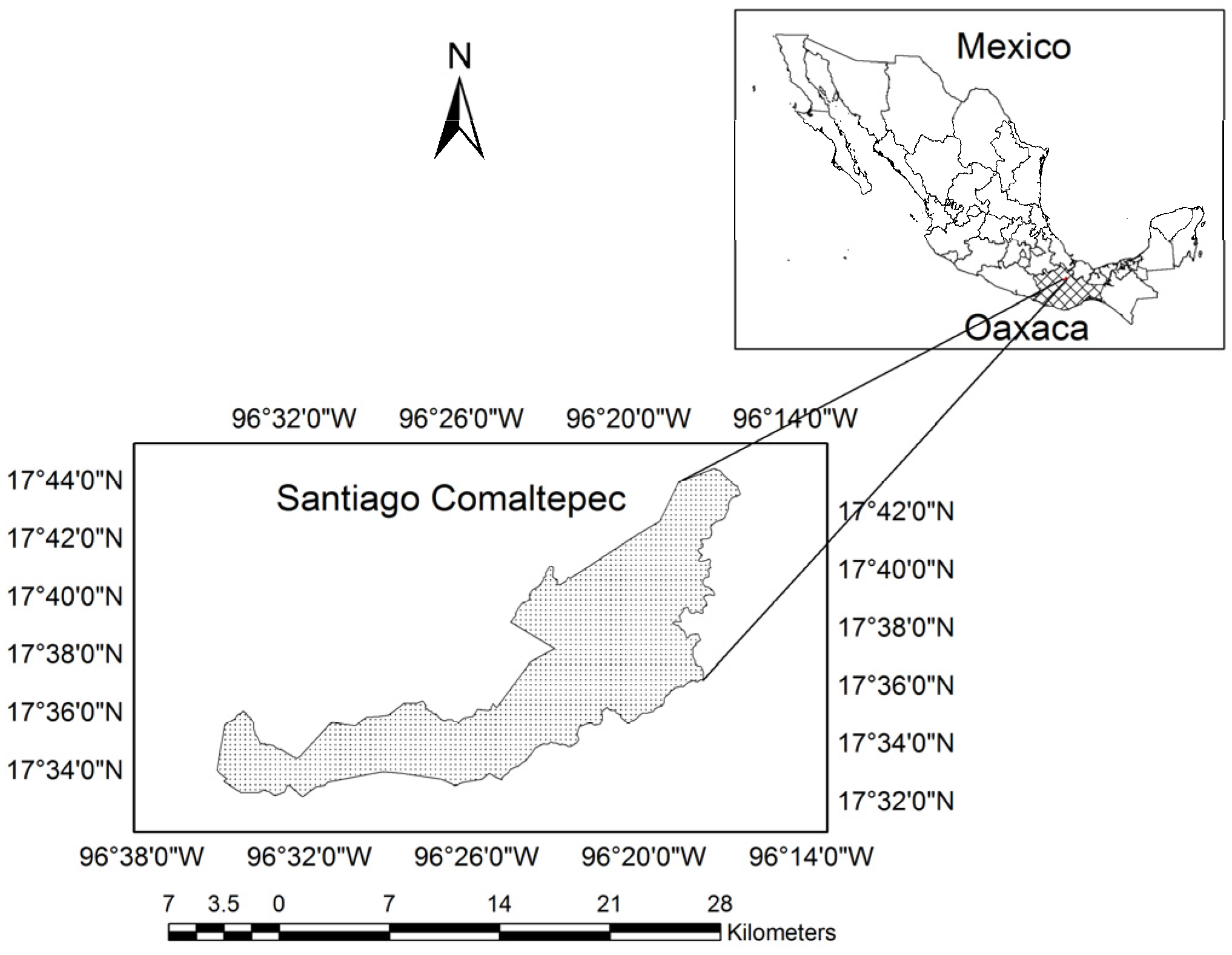
2.1. Study Area
2.2. Variables and Sample
2.3. Data Analysis
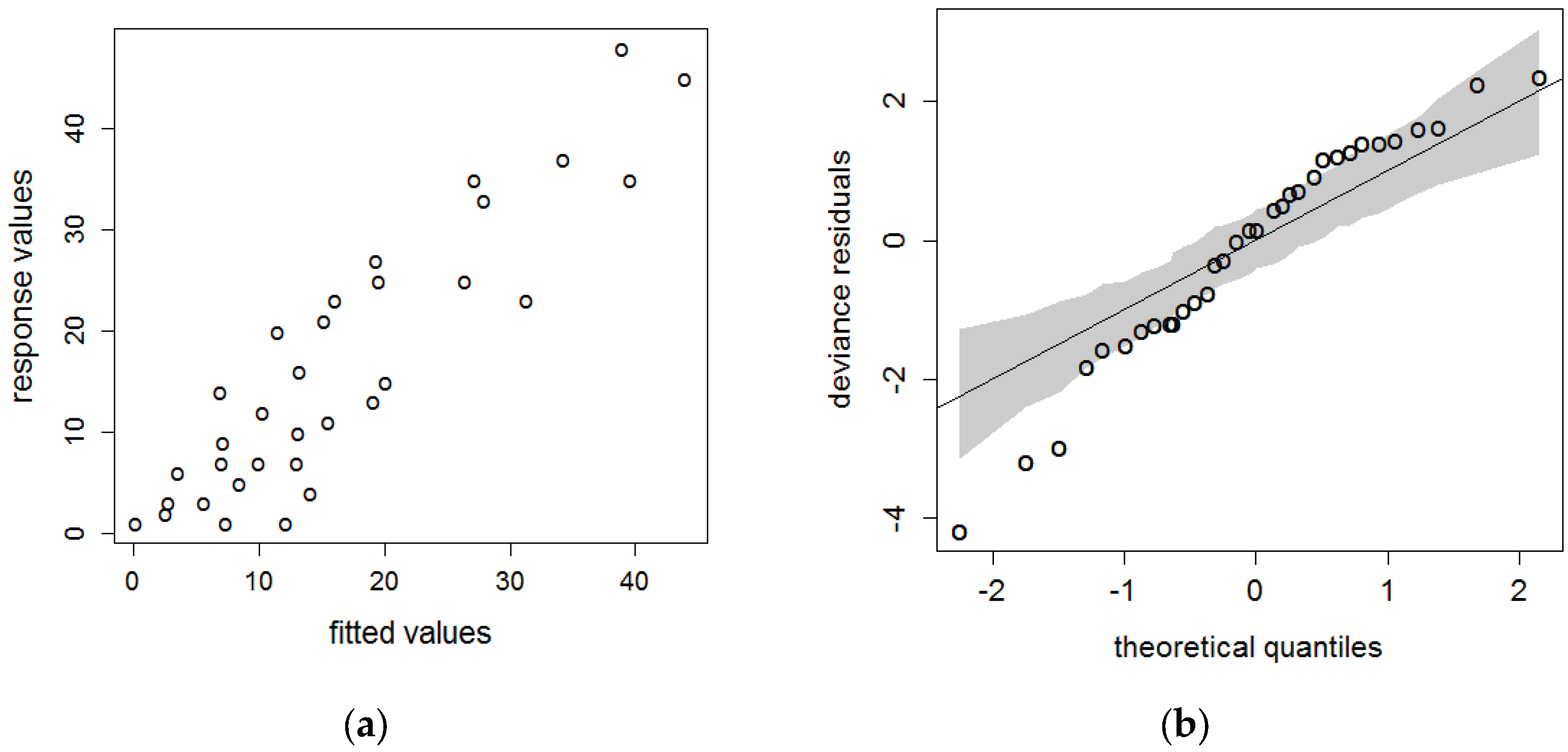
3. Results
4. Discussion
5. Conclusions
Acknowledgments
Author Contributions
Conflicts of Interest
References
- Guisan, A.; Edwards, T.C.; Hastie, T. Generalized linear and generalized additive models in studies of species distributions: Setting the scene. Ecol. Model. 2002, 157, 89–100. [Google Scholar] [CrossRef]
- Carrascal, L.M.; Bautista, L.M.; Lázaro, E. Geographical variation in the density of the white stork Ciconia ciconia in Spain: Influence of habitat structure and climate. Biol. Conserv. 1993, 65, 83–87. [Google Scholar] [CrossRef]
- Pliscoff, P.; Fuentes-Castillo, T. Modelación de la distribución de especies y ecosistemas en el tiempo y en el espacio: Una revisión de las nuevas herramientas y enfoques disponibles. Rev. Geogr. Norte gd. 2011, 48, 61–79. [Google Scholar] [CrossRef]
- Cade, B.S.; Noon, B.R. A gentle introduction to quantile regression for ecologists. Front. Ecol. Environ. 2003, 1, 412–420. [Google Scholar] [CrossRef]
- Weiher, E. Species richness along multiple gradients: Testing a general multivariate model in oak savannas. Oikos 2003, 101, 311–316. [Google Scholar] [CrossRef]
- Kass, G.V. An exploratory technique for investigating large quantities of categorical data. J. R. Stat. Soc. Ser. C 1980, 29, 119–127. [Google Scholar] [CrossRef]
- Olden, J.D.; Lawler, J.J.; Poff, N.L. Machine learning methods without tears: A primer for ecologists. Q. Rev. Biol. 2008, 83, 171–193. [Google Scholar] [CrossRef] [PubMed]
- Hastie, T.; Tibshirani, R. Generalized additive models. Stat. Sci. 1986, 1986, 297–310. [Google Scholar] [CrossRef]
- Nelder, J.; Wedderburn, R. Generalized Linear Models. J. R. Stat. Soc. Ser. A 1972, 135, 370–384. [Google Scholar] [CrossRef]
- Wood, S. Generalized Additive Models: An Introduction with R; Chapman Hall/CRC: Boca Raton, FL, USA, 2006; pp. 1–33. [Google Scholar]
- Wang, L.; Liu, X.; Liang, H.; Carroll, R.J. Estimation and variable selection for generalized additive partial linear models. Ann. Stat. 2011, 39. [Google Scholar] [CrossRef]
- McCullagh, P.; Nelder, J.A. Generalized Linear Models; Chapman and Hall: London, UK, 1989; p. 511. [Google Scholar]
- Nicholls, A.O. How to make biological surveys go further with generalised linear models. Biol Conserv. 1989, 50, 51–75. [Google Scholar] [CrossRef]
- Jaberg, C.; Guisan, A. Modelling the distribution of bats in relation to landscape structure in a temperate mountain environment. J. Appl. Ecol. 2001, 38, 1169–1181. [Google Scholar] [CrossRef]
- Elith, J.; Graham, J.C.H.; Anderson, P.; Zimmermann, N.E. Novel methods improve prediction of species’ distributions from occurrence data. Ecography 2006, 29, 129–151. [Google Scholar] [CrossRef]
- Maravelias, C.D. Trends in abundance and geographic distribution of North Sea herring in relation to environmental factors. Mar. Ecol. Prog. Ser. 1997, 159, 151–164. [Google Scholar] [CrossRef]
- Murase, H.; Nagashima, H.; Yonezaki, S.; Matsukura, R.; Kitakado, T. Application of a generalized additive model (GAM) to reveal relationships between environmental factors and distributions of pelagic fish and krill: A case study in Sendai Bay, Japan ICES. Afr. J. Mar. Sci. 2009, 66, 1417–1424. [Google Scholar] [CrossRef]
- CNA, Comisión Nacional del Agua. Servicio Meteorológico Nacional. Available online: http://smn.cna.gob.mx (accessed on 7 January 2016).
- INEGI, Instituto Nacional de Estadística y Geografía. Available online: http://www.beta.inegi.org.mx/app/mapa/espacioydatos/default.aspx (accessed on 8 January 2016).
- Schweik, C.M. Social norms and human foraging: An Investigation into the spatial distribution of Shorea Robusta in Nepal. Forest, Trees and People Programme. Available online: http://www.treesforlife.info/fao/Docs/P/X2104E/X2104E06.htm (accessed on 17 Octuber 2016).
- CONAFOR, Comisión Nacional Forestal, Sistema de Planeación Forestal Para Bosque Templado (SIPLAFOR). Available online: http://fcfposgradoujedmx/spf/inicio/documentosphp (accessed on 7 September 2016).
- Muñoz-Flores, H.J.; Sáenz-Reyes, J.; García-Sánchez, J.J.; Hernández-Máximo, E.; Anguiano Contreras, J. Áreas potenciales para establecer plantaciones forestales comerciales de Pinus pseudostrobus Lindl. y Pinus greggii Engelm. en Michoacán. Rev. Mex. Cienc. For. 2011, 2, 29–44. [Google Scholar]
- Nadezda, M.T.; Gerald, E.R.; Elena, I.P. Impacts of climate change on the distribution of Larix spp. and Pinus sylvestris and their climatypes in Siberia. Mitig. Adapt. Strateg. Glob. 2006, 11, 861–882. [Google Scholar] [CrossRef]
- Sáenz-Romero, C.; Rehfeldt, G.E.; Crookston, N.L.; Duval, P.; St-Amant, R.; Beaulieu, J.; Richardson, B.A. Spline models of contemporary, 2030, 2060 and 2090 climates for Mexico and their use in understanding climate-change impacts on the vegetation. Clim. Chang. 2010, 102, 595–623. [Google Scholar] [CrossRef]
- Martínez-Antúnez, P.; Hernández-Díaz, J.C.; Wehenkel, C.; López-Sánchez, C.A. Estimación de la densidad de especies de coníferas a partir de variables ambientales. Madera Bosques 2015, 21, 23–33. [Google Scholar] [CrossRef]
- Martínez-Antúnez, P.; Wehenkel, C.; Hernández-Díaz, J.C.; Corral-Rivas, J.J. Use of the Weibull function to model maximum probability of abundance of tree species in northwest Mexico. Ann. For. Sci. 2015, 72, 243–251. [Google Scholar] [CrossRef]
- Rehfeldt, G.E.; Crookston, N.L.; Warwell, M.V.; Evans, J.S. Empirical analyses of plants climate relationships for the western United States. Int. J. Plant Sci. 2006, 167, 1123–1150. [Google Scholar] [CrossRef]
- Crookston, N.L.; Rehfeldt, G.E.; Ferguson, D.E.; Warwell, M. FVS and Global Warming: A Prospectus for Future Development. Available online: http://www.treesearch.fs.fed.us/pubs/30963 (accessed on 1 June 2016).
- Sáenz-Romero, C.; Rehfeldt, G.E.; Ortega-Rodríguez, J.M.; Marín-Togo, M.C.; Madrigal-Sánchez, X. Pinus leiophylla suitable habitat for 1961–1990 and future climate. Bot. Sci. 2015, 93, 709–718. [Google Scholar] [CrossRef]
- Chapela, F. El Manejo Forestal Comunitario Indígena en la Sierra de Juárez, Oaxaca Los Bosques Comunitarios de México Manejo Sustentable de Paisajes Forestales. Available online: http://www2ineccgobmx/publicaciones/libros/532/cap5pdf (accessed on 17 September 2016).
- Guisan, A.; Graham, C.H.; Elith, J.; Huettmann, F. Sensitivity of predictive species distribution models to change in grain size. Divers. Distrib. 2007, 13, 332–340. [Google Scholar] [CrossRef]
- Austin, M. Species distribution models and ecological theory: A critical assessment and some possible new approaches. Ecol. Mod. 2007, 200, 1–19. [Google Scholar] [CrossRef]
- Meynard, C.N.; Quinn, J.F. Predicting species distributions: A critical comparison of the most common statistical models using artificial species. J. Biogeogr. 2007, 34, 1455–1469. [Google Scholar] [CrossRef]
- Dormann, F.C.; McPherson, J.M.; Araújo, M.B.; Kühn, I. Methods to account for spatial autocorrelation in the analysis of species distributional data: A review. Ecography 2007, 30, 609–628. [Google Scholar] [CrossRef]
- Canty, A.; Ripley, B. Package ‘Boot’. Available online: https://cranr-projectorg/web/packages/boot/bootpdf (accessed on 17 March 2016).
- Maindonald, J. Package ‘Gamclass’. Available online: https://cranr-projectorg/web/packages/gamclass/gamclasspdf (accessed on 7 August 2016).
- McCulloch, C.E. Generalized linear models. J. Am. Stat. Assoc. 2000, 95, 1320–1324. [Google Scholar] [CrossRef]
- Hochberg, Y. A sharper Bonferroni procedure for multiple tests of significance. Biometrika 1988, 75, 800–802. [Google Scholar] [CrossRef]
- Bio, A.M.F.; Alkemade, R.; Barendregt, A. Determining alternative models for vegetation response analysis: A non-parametric approach. J. Veg. Sci. 1998, 9, 5–16. [Google Scholar] [CrossRef]
- Lehmann, A. GIS modeling of submerged macrophyte distribution using Generalized Additive Models. Plant Ecol. 1998, 139, 113–124. [Google Scholar] [CrossRef]
- Austin, M.P. Spatial prediction of species distribution: An interface between ecological theory and statistical modeling. Ecol. Model. 2002, 157, 101–118. [Google Scholar] [CrossRef]
- Craven, P.; Wahba, G. Smoothing Noisy Data with Spline Functions Estimating the Correct Degree of Smoothing by the Method of Generalized Cross-Validation Numerische. Mathematik 1978, 31, 377–404. [Google Scholar] [CrossRef]
- Wood, S.N. Fast stable restricted maximum likelihood and marginal likelihood estimation of semiparametric generalized linear models. J. R. Stat. Soc. B Met. 2011, 73, 3–36. [Google Scholar] [CrossRef] [Green Version]
- Rodríguez-Rivera, V.; Alfonso-Corrado, C.; Aguirre-Hidalgo, A.; Campos, J.E.; Venegas-Barrera, C.S.; Clark-Tapia1, R. Galls and host occurrences along a forest gradient in Sierra Juárez, Oaxaca, Mexico. J. Environ. Biol. 2017, 38, 1–7. [Google Scholar] [CrossRef]
- Hunter, P. The human impact on biological diversity. EMBO Rep. 2007, 8, 316–318. [Google Scholar] [CrossRef] [PubMed]
- Crowther, T.W.; Glick, H.B.; Covey, K.R.; Bettigole, C.; Maynard, D.S.; Thomas, S.M.; Smith, J.R.; Hintler, G.; Duguid, M.C.; AmatullI, G.; et al. Mapping tree density at a global scale. Nature 2015, 525, 201–205. [Google Scholar] [CrossRef] [PubMed]
- Sáenz-Romero, C.; Martínez-Palacios, A.; Gómez-Sierra, J.M.; Pérez-Nasser, N.; Sánchez-Vargas, N.M. Estimación de la disociación de Agave cupreata a su hábitat idóneo debido al cambio climático. Rev. Chapingo Ser. Cien. 2012, 18, 291–301. [Google Scholar]
- Oreskes, N.; Shrader-Frechette, K.; Belitz, K. Verification, validation, and confirmation of numerical models in the earth sciences. Science 1994, 263, 641–646. [Google Scholar] [CrossRef] [PubMed]
- Seoane, J.; Bustamante, J. Modelos predictivos de la distribución de especies: Una revisión de sus limitaciones. Ecología 2001, 15, 9–21. [Google Scholar]
- Rehfeldt, G.E.; Crookston, N.L.; Sáenz-Romero, C.; Campbell, E.M. North American vegetation model for land-use planning in a changing climate: A solution to large classification problems. Ecol. Appl. 2012, 22, 119–141. [Google Scholar] [CrossRef] [PubMed]
- Zhu, Q.; Jiang, H.; Liu, J.; Peng, C.; Fang, X.; Yu, S.; Zhou, G.; Wei, X.; Ju, W. Forecasting carbon budget under climate change and CO2 fertilization for subtropical region in China using Integrated Biosphere Simulator (IBIS) model. Pol. J. Ecol. 2011, 59, 3–23. [Google Scholar]
- Desai, A.R.; Normets, A.; Bolstad, P.V.; Chen, J.; Cook, B.D.; Davis, K.J.; Euskirchen, E.S.; Gough, C.; Martin, J.G.; Ricciuto, D.M.; et al. Influence of vegetation and seasonal forcing on carbon dioxide fluxes across the Upper Midwest, USA: Implications for regional scaling. Agric. For. Meteorol. 2008, 148, 288–308. [Google Scholar] [CrossRef]
- Goparaju, L.; Jha, C.S. Spatial dynamics of species diversity in fragmented plant communities of a Vindhyan dry tropical forest in India. Trop. Ecol. 2010, 51, 55–65. [Google Scholar]
- Austin, M.P.; Belbin, L.; Meyers, J.A.; Doherty, M.D.; Luoto, M. Evaluation of statistical models used for predicting plant species distributions: Role of artificial data and theory. Ecol. Mod. 2006, 199, 197–216. [Google Scholar] [CrossRef]
- Raxworthy, C.J.; Martinez-Meyer, E.; Horning, N.; Nussbaum, R.A.; Schneider, G.E.; Ortega-Huerta, M.A.; Peterson, A.T. Predicting distributions of known and unknown reptile species in Madagascar. Nature 2003, 426, 837–841. [Google Scholar] [CrossRef] [PubMed]
- Martínez-Meyer, E.; Peterson, A.T. Conservatism of ecological niche characteristics in North American plant species over the Pleistocene to Recent transition. J. Biogeogr. 2006, 33, 1779–1789. [Google Scholar] [CrossRef]
- Ward, M.D.; Gleditsch, K.S. Spatial Regression Models. 2008. Available online: http://us.corwin.com/sites/default/files/upm-binaries/21130_Chapter_11.pdf (accessed on 19 January 2017).
- Le Gallo, J. Cross-section spatial regression models. In Handbook of Regional Science; Fischer, M.M., Nijkamp, P., Eds.; Springer: Berlin, Germany, 2014; pp. 1511–1533. [Google Scholar]


| Quercus macdougallii | AR | AST | ASP | ELEV | AI | GSP | MTCM | MTWM | FFP | SMRSPRPB | SPRP | |
| Maximum | 48 | 90 | 9 | 2968 | 0.047 | 2144 | 13.5 | 18.5 | 364 | 5.9 | 168 | |
| Minimum | 1 | 10 | 2 | 2001 | 0.014 | 1024 | 7.8 | 12.1 | 208 | 5.2 | 84 | |
| SD | 14.4 | 28.1 | 2.4 | 530.3 | 0.009 | 432 | 2.3 | 3 | 65.5 | 1 | 33.6 | |
| Mean | 17.6 | 32.3 | 6.9 | 2649.2 | 0.024 | 1615.5 | 9.6 | 13.8 | 264.7 | 5.6 | 129.8 | |
| Pinus patula | AR | AST | ASP | ELEV | AI | MAP | GSP | MMIN | DD5 | D100 | SMRP | |
| Maximum | 185 | 95 | 9 | 3002 | 0.047 | 3063 | 2220 | 7.4 | 3906 | 32 | 1019 | |
| Minimum | 1 | 10 | 1 | 2001 | 0.013 | 1318 | 1022 | 2.9 | 1699 | 12 | 447 | |
| SD | 29.7 | 23.5 | 2.5 | 224.4 | 0.007 | 441.1 | 304.2 | 0.9 | 403.3 | 4.5 | 145.6 | |
| Mean | 21.8 | 38.4 | 5.9 | 2635.9 | 0.024 | 2140.1 | 1581.8 | 4.5 | 2322.8 | 22.1 | 709.7 | |
| Pinus pseudostrobus | AR | AST | ASP | ELEV | AI | MAT | GSP | MTWM | MMAX | D100 | WINP | |
| Maximum | 174 | 95 | 360 | 3002 | 0.048 | 15.9 | 2220 | 18.7 | 25.3 | 32 | 441 | |
| Minimum | 1 | 10 | 1 | 1983 | 0.013 | 9.5 | 1016 | 12 | 17.4 | 12 | 157 | |
| SD | 26.7 | 24 | 116 | 226.2 | 0.007 | 1.113 | 302.7 | 1.0977 | 1.329 | 4.535329 | 69.54 | |
| Mean | 16.9 | 44 | 207 | 2613 | 0.024 | 11.39 | 1564 | 13.666 | 19.55 | 21.79208 | 291.6 |
| Predictors | Quercus macdougallii | Pinus patula | Pinus pseudostrobus | |||||||||
|---|---|---|---|---|---|---|---|---|---|---|---|---|
| GLM | GAM | GLM | GAM | GLM | GAM | |||||||
| Parms | p-Values | EDF | p-Values | Parms | p-Values | EDF | p-Values | Parms | p-Values | EDF | p-Values | |
| Intercept | 7.724 | <0.001 * | 2.6 | <0.001 * | 10.21 | <0.001 * | 2.8 | <0.001 * | 15.89 | <0.001 * | 2.6 | <0.001 * |
| AST | −0.002 | 0.430 | 2.8 | <0.001 * | −0.002 | <0.001 * | 4.0 | <0.001 * | 0.004 | <0.001 * | 7.6 | <0.001 * |
| ASP | 0.032 | 0.125 | 2.4 | <0.001 * | 0.068 | <0.001 * | 2.0 | <0.001 * | 0.001 | 0.489 | 4.9 | <0.001 * |
| GSP | −0.002 | 0.001 * | 1.9 | <0.001 * | −0.002 | <0.001 * | 4.0 | <0.001 * | −0.004 | <0.001 * | 4.9 | <0.001 * |
| AI | −84.66 | <0.001 * | 1.0 | <0.001 * | −168 | <0.001 * | 5.0 | <0.001 * | −265.3 | <0.001 * | 4.9 | <0.001 * |
| SME | 250.29 | 322.59 | 810.15 | 774.45 | 686.91 | 706.6 | ||||||
| DE | 8.8 | 46.9 | 14.08 | 25.6 | 11.45 | 20.3 | ||||||
| AIC | 469.9 | 346.5 | 9825.7 | 8705.3 | 7540.3 | 7725.2 | ||||||
| Quercus macdougallii | Pinus patula | Pinus pseudostrobus | ||||||||||
|---|---|---|---|---|---|---|---|---|---|---|---|---|
| COV | Model Type | DE | EDF | p-Values | COV | DE | EDF | p-Values | COV | DE | EDF | p-Values |
| AST | M | 3.3 | 0.0019 * | AST | 3.8 | <0.001 * | AST | 7.7 | <0.001 * | |||
| S | 14.2 | 3.7 | 1.3 | 4.6 | 3.5 | 4.8 | ||||||
| ASP | M | 2.3 | 0.0003 * | ASP | 1.9 | <0.001 * | ASP | 5 | <0.001 * | |||
| S | 3.8 | 1.9 | 6.3 | 4.9 | 4.4 | 4.9 | ||||||
| ELEV | M | 3.8 | 0.0015 * | ELEV | 4.5 | <0.001 * | ELEV | 4.8 | <0.001 * | |||
| S | 15.5 | 3.6 | 18.4 | 4.9 | 10.7 | 4.8 | ||||||
| GSP | M | 1 | 0.4694 | MAP | 3.0 | <0.001 * | WINP | 4.9 | <0.001 * | |||
| S | 23.6 | 4.9 | 17.5 | 4.9 | 11.0 | 3.9 | ||||||
| SPRP | M | 1.9 | 0.0291 | GSP | 4.0 | <0.001 * | D100 | 4.1 | <0.001 * | |||
| S | 23.8 | 4.9 | 17.8 | 5.0 | 9.7 | 4.6 | ||||||
| SMRSPRPB | M | 1.2 | 0.5672 | SMRP | 1.9 | <0.001 * | GSP | 5 | <0.001 * | |||
| S | 8.3 | 4.8 | 18.1 | 4.9 | 11.1 | 4.9 | ||||||
| MTCM | M | 3.9 | 0.0221 | DD5 | 1.6 | <0.001 * | MMAX | 4.9 | <0.001 * | |||
| S | 24.7 | 4.9 | 17.6 | 4.9 | 11.2 | 4.8 | ||||||
| MTWM | M | 2 | 0.0400 | D100 | 1.9 | <0.001 * | MAT | 4.1 | <0.001 * | |||
| S | 24.1 | 4.9 | 18.0 | 10.8 | 4.7 | |||||||
| FFP | M | 1.9 | <0.001 * | MMIN | 4.8 | <0.001 * | MTWM | 4.9 | <0.001 * | |||
| S | 18.9 | 4.3 | 18.6 | 4.9 | 11.0 | 4.7 | ||||||
| INTERCEPT (M) | 2.5 | 2.8 | 2.5 | |||||||||
| AIC (M) | 266 | 7940.5 | 6821 | |||||||||
| SME (M) | 3462 | 7596 | 7008 | |||||||||
| DE (M) | 76.8 | 33.6 | 31.9 | |||||||||
| UBRE (M) | 2.84 | 19.70 | 17.69 | |||||||||
© 2017 by the authors. Licensee MDPI, Basel, Switzerland. This article is an open access article distributed under the terms and conditions of the Creative Commons Attribution (CC BY) license ( http://creativecommons.org/licenses/by/4.0/).
Share and Cite
Antúnez, P.; Hernández-Díaz, J.C.; Wehenkel, C.; Clark-Tapia, R. Generalized Models: An Application to Identify Environmental Variables That Significantly Affect the Abundance of Three Tree Species. Forests 2017, 8, 59. https://doi.org/10.3390/f8030059
Antúnez P, Hernández-Díaz JC, Wehenkel C, Clark-Tapia R. Generalized Models: An Application to Identify Environmental Variables That Significantly Affect the Abundance of Three Tree Species. Forests. 2017; 8(3):59. https://doi.org/10.3390/f8030059
Chicago/Turabian StyleAntúnez, Pablo, José Ciro Hernández-Díaz, Christian Wehenkel, and Ricardo Clark-Tapia. 2017. "Generalized Models: An Application to Identify Environmental Variables That Significantly Affect the Abundance of Three Tree Species" Forests 8, no. 3: 59. https://doi.org/10.3390/f8030059
APA StyleAntúnez, P., Hernández-Díaz, J. C., Wehenkel, C., & Clark-Tapia, R. (2017). Generalized Models: An Application to Identify Environmental Variables That Significantly Affect the Abundance of Three Tree Species. Forests, 8(3), 59. https://doi.org/10.3390/f8030059