Relationship between Forest Color Characteristics and Scenic Beauty: Case Study Analyzing Pictures of Mountainous Forests at Sloped Positions in Jiuzhai Valley, China

Abstract

Forests are important place for outdoor recreation and scenery appreciation. So in order to better meet the needs of the public, forest appreciation has received increasing attention from foresters in recent years. However, related research is still limited. Therefore, this paper seeks to examine the relationship between forest colors (measured by specific elements and spatial indices of color) and Scenic Beauty Estimation values. We researched Jiuzhai Valley in China by selecting 104 pictures to determine the scenic beauty estimation values of forests in a mountainous region. Quantitative color elements were extracted by programming on Matlab, and spatial indices of color patches were extracted by ArcGIS and FRAGSTATS. A total of 23 indices were obtained to explain the color characteristics of each forest picture. The results showed that the yellow and red colors were the main mutable colors of Jiuzhai Valley in autumn, but the color patches index had no significant change over time in that season. After partial correlation analysis, principal component analysis, and cluster analysis, we found that 14 color elements, eight color patch factors and six particular indices had an effect on the SBE values, which can then be used to efficiently measure and enhance the forest color beauty of Jiuzhai Valley.

1. Introduction

Forests play a crucial role in relieving the population from the effects of urbanization, allowing visitors to get closer to nature and to restore their bodies and mind. Therefore, based on their ecological functions, forests have become a research hotspot with respect to improving their service value. Some research shows that improving scenic beauty is effective, and that the color of plants is an important effective indicator [1]. Color is a visual characteristic triggered by light and differing from spatial attributes. It stimulates human visual nerves more than other factors such as the shape, size, etc. [2]. Plant color has a relatively obvious effect on the transmission of forest visual characteristics and the stimulation of the human sensory apparatus. In China, many ecological forests have started to introduce an increasing number of flowering and discoloring species during the transformation process. However, there is little research into the relationship between forest colors and scenic beauty. Such research can provide a scientific basis for the management and operation of forest sceneries by assessing and analyzing the relationship between forest color indices and scenic beauty values, and it can help foresters to carry out tending work that meets the public’s aesthetic needs.

The aesthetic analysis of a single color is common among color studies [3]. However, the color definition of an individual plant is still unclear in color aesthetics. For example, a yellow daffodil is often regarded as a type of green plant by people. Moreover, different populations have aesthetic differences with respect to individual plants [4]. In practical applications, the aesthetic experience of plant colors is only applicable to guiding the configuration of individual trees, and its application range is limited. Currently, aesthetic studies of single plants are almost entirely absent. Rather, research is mainly carried out on the color composition of more complex plant groups, and these mostly focus on the community color at middle or small scales.

At present, research into community colors and public aesthetics proceed in two directions. The first direction involves a theoretical evaluation: viz., color harmony theory. Color harmony is the theoretical system for exploring the relationship among different colors based on an aesthetic view. The relationship between the adjacent color, contrast colors, and similar colors can be used to select plant color configuration modes for better scenery [5]. Color harmony theory is usually applied to the evaluation of several color combinations, and requires the recognition of main colors to determine the visual relationship between colors. For example, contrast colors such as red and green of plants in autumn can stimulate vision, while adjacent colors such as red and yellow plants can make a landscape look modest. Therefore, color harmony theory is mostly used to determine the color configurations of plants on a small scale or with fewer species. In recent years, some scholars relied on the following claim: “when mixed colors turn to neutral grey, they are symbols of color harmony.” This hypothesis is central to the Munsell Color System for optimizing the color of plant communities [6]. That is to say, through replanting and thinning, when the values of brightness and saturation are both 50% in the forest landscape, the scenery is said to be harmonized in terms of its overall color. Since then, some scholars have used the same methods to obtain an optimized landscape, by issuing questionnaires based on it. The results showed that landscape optimization under the guidance of color harmony theory had a demonstrable and positive effect on the public [7]. However, the theory of color harmony is based on aesthetics, which are easily affected by social factors such as human history, geography, and culture [8]. Consequently, it has a certain bias as a measurement standard for color aesthetics.

The second direction is quantitative: viz., scenic beauty estimations. This approach involves judging the level of beauty by having the public or experts score the landscape [9]. This direction pays more attention to the public’s aesthetic responses and population differences. Scenic beauty research has long been carried out and at this point has a mature theoretical and practical basis [10]. The Scenic Beauty Estimation (SBE) and Law of Comparative Judgment (LCJ) methods are the most commonly used [9,11]. However, these evaluation systems usually score the overall factors combining the community structure, canopy characteristics, plant morphology, seasonal changes, environmental quality, and more. Usually, the color factor is just a small part. As such, there is a lack of in-depth studies regarding the relationship between plant colors and aesthetics, and researchers have failed to sufficiently understand how color compositions affect aesthetics. Recently, some studies in China began to discuss the impact of different plant colors on SBE scoring. These studies took the proportion of plant colors, color layout, etc. as their focus. In a study of color composition, Li found that when the area ratio of Amygdalus davidiana Carr. and other green trees was 2:1 and the distribution of Amygdalus davidiana was comprehensive or intensive, the community had the largest SBE value [12]. In the single tree color preferences research, Sun found yellow hue, high brightness and value were related to high beauty scores of yellow trees, and brightness and saturation were not related to the beauty scores of brown trees in any way; red trees were the same as yellow ones in terms of their beauty [13]. Recently, the field of plant color aesthetic research has been extended. Furthermore, the extraction of plant color factors has been continually enriched. Yet, aesthetic evaluations have always been implemented using only two types of methods: color harmony theory and SBE. Among these, SBE is better recognized for its advantages of quantity and demographic distinction.

In general, a qualitative method is the most common way to research forest color aesthetics, mostly using type variables to explain forest colors. Nevertheless, the results are not sufficiently precise. This is mainly related to the development of plant color measurement methods. At present, there are three main methods for quantifying color elements. One is the visual control method: researchers use color cards to compare plant colors and derive the closest color value. This is mainly applied in plant color research with few colors or low precision [10,14]. The second is the instrument measurement method. This method uses a color measuring spectrometer to measure the plant. The method is highly precise, but requires very close distance. Thus, it can only measure the color value at a certain point, and is suitable only for measuring the color of partial plant organs [15]. The third method is a software quantification method. It uses a digital camera to record forest colors, and combines Photoshop [16], ColorImpact [17] and other software for image processing, thus quantifying color elements. It is suitable for forest landscapes with multiple colors or on a large scale. Furthermore, this method is significantly affected by the environment, light, observation distances, camera sensor performance, and other factors. It requires removing non-plant factors in the image to reduce the influence of these colors [13].

In summary, forest colors are an important component to the quality of forest landscapes and to the aesthetic needs of the public. The study of color and forest scenic beauty is both theoretical and practical. This study is aimed at surveying forest color beauty at a relatively large scale, namely the landscape in Jiuzhai Valley, China. That is to say, we try to examine what types of color characteristics are related to public aesthetic preferences. Our method of image data acquisition is described, and the quantization of the color elements is explored under the mode of self-programming. Then, after combining the color patch space indices, we obtained all the factors of forest color, after that the relationship of these factors and SBE values is analyzed. Using our method, we hope to provide some suggestions for forest scenery management with similar plant species.

2. Materials and Methods

2.1. Study Area

Jiuzhai Valley in northern Sichuan is the first nature reserve in China to have as its primary goal the preservation of its natural scenery. It is also a tourist destination with the concurrent titles UNESCO World Natural Heritage Site, National Key Scenic Spot, and National and Scenic National Park. It has important value in terms of tourism, with over 5 million visitors in 2016. It has an average altitude of 3000 meters and forest coverage rate of more than 80%. The research sites we selected included mountainous landscapes with natural secondary forests, and with a certain proximity to tourists. The dominant community types are Betula Linn., Alibes Mill., Quercus Linn., Picea wilsonii Mast., Pinus tabuliformis Carr., and Picea Dietr. Various types of plants change color in autumn, when the foliage ultimately results in a colorful forest scene of yellow and red.

2.2. Sampling Area Selection

Based on the primary survey of the forest landscape of Jiuzhai Valley and typical sampling methods, we chose 57 observing sites on three main tourist lines. Essential information from each sample plot was measured and recorded (

Table 1. Essential information of sample plots.

Slope Direction	Percent (%)	Altitude (m)	Distance (m)	Height (m)	Height Angle (degree)
East	1.8	2648 ± 0	211 ± 0	162.5 ± 0	37.6 ± 0
Northeast	21.8	2453 ± 230	278 ± 115	121.9 ± 63.7	23.9 ± 7.2
Northwest	10.9	2665 ± 264	253 ± 116	146.4 ± 77.6	28.8 ± 5.1
South	9.1	2483 ± 139	285 ± 150	79.8 ± 51.0	17.3 ± 7.1
Southeast	12.7	2525 ± 279	254 ± 56	120.8 ± 68.6	24.1 ± 13.2
Southwest	43.6	2476 ± 208	234 ± 75	121.8 ± 54.8	27.1 ± 7
Total	100	2501 ± 223	252 ± 94	121 ± 60.3	25.5 ± 8.3

). Longitude, latitude, and altitude were measured with a GPS instrument (Garmin Montana 650), the height and distance of the mountains were surveyed using a laser range finder, a compass was used to ascertain the direction of slopes, and a digital light meter was used to measure the illumination intensity at corresponding periods. The weather situation and species composition were also recorded.

2.3. Photography

It was verified in previous studies that the real landscape could be depicted well and truly using colorized photos [18]. Furthermore, when the image was larger, image analysis was more efficacious than any other color extraction method. Nonetheless, photo quality and detail were always affected by environmental factors such as illumination intensity, air quality, and other factors (tourists or buildings, etc.). Thus, standard operations must be performed to minimize the influential factors during image acquisition and picture processing [19]. All pictures were collected with a Canon EOS-7D with 18 million pixels under bright illumination between 10 a.m. and 3 p.m. We acquired the images on three occasions in 2015: 28 August, 28 September, and 27 October. To guarantee the key characteristics, we attempted to omit all elements except the forest landscape, and shooting positions, angles, and modes were unified each time. In total, 171 pictures were collected. We then removed those that were heavily defoliated or affected by environmental factors, leaving us with a total of 104 photos. To avoid the effects of different sky colors in each picture, Adobe Photoshop CC software was used to change the sky color of every image into two forms. One form was the change to pure white for color quantization, and the pure white can be deleted easily in the color element extraction, so as to eliminate the influence of sky color. The other form was changing to identical blue with the same white clouds for the sake of aesthetic value, so that the preferred influence of sky can be deleted (Figure 1).

2.4. Scenic Beauty Estimation and Dependability Control

SBE is generally used in forests and other landscape investigations, in addition to simple surveys. It is more important that the standardized SBE values can effectively reduce deviation caused by individual variation [18]. Consequently, SBE was adopted to evaluate the forest color landscapes in Jiuzhai Valley using image questionnaires.

There is no definition of the population in this paper, and random samplings were taken for the survey. Many researchers discussed how to choose a sample size from different targets. Nei considered that 381 samples would be suitable for a 95% confidence coefficient when the statistical population was sufficiently large [20]; Creswell utilized attributes of questionnaire surveys, and suggested that the number of formal samples should be more than 350 [21]. This study confirmed the sample size using the formula from Scheaffer [22]:

$$n=\frac{N}{\left(N-1\right){\delta }^2+1}$$

(1)

where n is the sample number, N is the statistical population, and δ is the sample error (here, 0.05). That is, the confidence coefficient equals 95%. In this study, the statistical population was sufficiently large, at n ≥ 400 after the calculations.

In consideration of the sample size, survey time, and people selected, the traditional interior multimedia playback mode was replaced with other methods, to improve the population structure of subjects and to guarantee the sample size. Polat printed pictures and surveyed some parks [23]; Schirpke used a network for research [24]. We adopted a Web-based survey, with the help of a questionnaire platform, and issued 600 questionnaires randomly, ultimately collecting 453 of these.

Table 2. Basic demographics of questionnaire subjects.

Basic Information	Category	Number	Percent (%)	Basic Information	Category	Number	Percent (%)
Gender	Men	231	50.7		Central China	28	6.1
	Women	225	49.3		South China	60	13.2
Age	Under 25 years old	58	12.7		Southwest China	56	12.3
	26–35 years old	190	41.7		Northwest China	12	2.6
	36–55 years old	171	37.5	Annual forest recreation times	0	15	3.3
	55 years old or older	37	8.1		1–3	142	31.1
Education	Primary education	11	2.4		4–10	174	38.2
	Junior education	89	19.5		11–20	87	19.1
	College	277	60.7		21–100	32	7.0
	Graduate	79	17.3		101–200	5	1.1
Region	North China	93	20.4		201 or more	1	0.2
	Northeast China	47	10.3	Work about forests?	Yes	49	10.7
	Eastern China	160	35.1		No	407	89.3

shows the basic demographics of the subjects.

The image order was determined randomly, and seven grades of beauty classification were chosen for all evaluators. All participants marked the pictures from −3 to 3, which represent a range from “not beautiful at all” to “most beautiful.” The language of the questionnaire, case description, and survey steps were determined based on the investigation standard of SBE by Daniel [25]. As a multiple scoring type, a reliability test can be used to judge the dependability of the image questionnaire. Therefore, we utilized the α-coefficient calculation method by Cronbach [12], with the following formula:

$$\alpha =\frac{k}{k-1}\left[1-\frac{{\sum }_{i=1}^k{S_i}^2}{{S_x}^2}\right]$$

(2)

where k is the number of survey pictures, S_i is the score variance of the ith question, and S_x is the score variance of all the pictures. There were 104 pictures in this study, after calculating α = 0.973, meaning that the reliability test succeeded.

2.5. Color Element Extraction

2.5.1. Color Quantization Based on the HSV Model

The most popular method of color quantization involves expressing the color information of digital images using color models. This method is widely used in computer image retrieval. Among the many color models, the Hue, Saturation, and Value (HSV) color space (see Figure S1a for more details) is comparatively closer to the color perception of human eyes. The distance between the two HSV color points in the color space can be calculated using the Euclidean distance. Thus, it is helpful to quantify colors that are consistent with human perception [26]. To facilitate quantification, usually three components of H, S, and V require respective and proper partitioning and classification to reduce the number of colors. However, when the image colors change slightly, this approach will result in a less clear attribution of color values near the category threshold. Therefore, in the color quantization, the choices of quantization classification and quantity are critical [27]. Smith extracted 166 colors in his study [28], and Zhang extracted 36 colors [26]. An excessive number of colors in quantization will increase the workload and change the sensitivity of the colors. However, if the number of quantification colors is too small, the research will lose a considerable amount of color information, ultimately deteriorating the accuracy of the quantification. This paper adopted Chen’s quantization methods, dividing the HSV color space into 256 colors. Here, H:S:V = 16:4:4 [27]. Then, we performed subsequent processing. At the same time, the true distribution of the color space is not uniform. Compared with the uniform quantization method, non-uniform color quantization can divide colors into the same groups more reasonably. This is suitable for the division of saturation and value by non-uniform color quantization [28,29] (see Figure S2 for more details). In total, 256 colors were obtained in this way. Any color that belonged to the same interval after the quantification was considered the same color.

However, some colors among the 256 quantified were difficult for human eyes to distinguish. So after non-uniform quantization, this study normalized similar colors into Black, White, and Grey (see more details in Figure S3), and then 147 colors were ultimately obtained by 144 colors (Figure 2) together with Black, White, and Grey. In Figure 2, we selected one representative color in the color classification threshold to fill each interval, but actually, each block represented a type of color range containing many colors within the threshold value. As shown in Figure 2, H1 and H2, belong to the red color, H3 and H4 belong to the yellow color, H5, H6, H7, H8, and H9 belong to the green color, and H10, H11, H12, H13, H14, H15, and H16 belong to the blue-violet color. Then, according to non-uniform quantization and color normalization processing described above, we completed the programming using the MATLAB2015a (Math Works) platform, by calculating the pixel value of each type of color in different images. The results were written into Excel 2013 (see more details in Figure S4). Figure 3 shows an example of an original pictures converted to a 147-color pattern by Matlab, thereby simplifying the colors in the photo.

2.5.2. Selection of Color Component Indicators

According to previous research, color attribute factors such as the ratio of main color, hue, saturation, and value were selected [17,19]. We selected five color indicators based on current research and the color characteristics of Jiuzhai Valley. The total pixels in the original images were the same. In this study, skies were classified as background and removed. Therefore, they were not included in the calculation. Consequently, the total number of pixels in each image was the number of pixels without sky pixels. When the proportion of color pixels was too small, the color was relatively difficult to recognize to the naked eye. To simplify the data, in this analysis, colors with a proportion of less than 1% were ignored. Based on the color quantization data obtained above, the quantitative calculation of each factor component indicators had been carried out.

• Hue Ratio (H): a total of sixteen hue ratios (H1, H2, H3, ..., H16), where $A_{H_i}$ is the sum of pixels of the ith hue; $A_n$ is the total number of pixels.

  $$H{P}_i=\frac{A_{H_i}}{A_n}\times 100$$

  (3)
• Saturation Ratio (S): five saturation proportions of S1, S2, S3, Grey, and White, where $A_{S_i}$ is the sum of pixels of the ith saturation interval; $A_n$ is the total pixels.

  $$S{P}_i=\frac{A_{S_i}}{A_n}\times 100$$

  (4)
• Value Ratio (V): four brightness ratios of Black, V1, V2, and V3, where $A_{V_i}$ is the sum of pixels of the ith value interval; $A_n$ is the total pixels.

  $$V{P}_i=\frac{A_{V_i}}{A_n}\times 100$$

  (5)
• Number of Colors (NC): among the 147 colors, the number of colors with a proportion of no less than 1%.

  $$\mathrm{NC}=\mathrm{SUM}\left(H_a{S}_b{V}_c\right), H_a{S}_b{V}_c{P}_i\ge 1\%$$

  (6)
• Maximum Hue Index (MHI): ratio of the hue with the largest pixel proportion, with the exception of Black and White.

  $$MHI=\frac{A_{MH}}{A_n}\times 100$$

  (7)

2.6. Spatial Index of Color Patches

We sketched color patches in ArcGIS (10.3, Esri, Redlands, CA, United States) by visual interpretation, and converted vector data to a grid. Then, with the help of FRAGSTATS (v4.2.1, University of Massachusetts, Amherst, MA, United States), spatial form indices of color patches were calculated. Pictures in this research were exclusively forest landscapes in mountainous slopes. These rules were adopted when determining the boundaries of the color patches. (1) We first demarcated the pictures based on different species of plants. From photos of Jiuzhai Valley, colors were distinct among evergreen coniferous forest and broadleaved deciduous forest. Therefore, distinguishing tree species was the first demarcation rule. (2) We demarcated the pictures based on color differences. In some pictures, there were various shrubwoods mixed together, making it difficult to distinguish them one-by-one. Thus, we relied on color differences, putting species with similar colors in one patch under normal visual discrimination. (3) We magnified photos with high definition, in order to reduce visual errors as much as possible.

Based on existing research results and the forest characteristics in Jiuzhai Valley [30], 18 categories were defined as follows: proportion of coniferous forest (AP), broad-leaved forest proportion (BP), shrubwood proportion (SP), total area of color patches (TA), color patch perimeter-area ratio (PARA), color diversity in patches (CD), color patch density (PD), largest color patch index (LPI), color landscape shape index (LSI), contagion of color patch (CON), landscape division index of color (DIV), splitting index of color patch (SPL), Shannon’s diversity index of color patch (SHDI), Simpson’s evenness index of color patch (SIEI), aggregation index of color patch (AI), proportion of alike adjacencies of color patch (PLA), color patch of cohesion index (COH), and the mean area proportion of the color patch (ARP).

2.7. Data Processing and Analysis

2.7.1. Standardized Calculation of SBE Value

Aesthetic measures invite differences between different respondents, affecting the evaluation results according to either strict or loose standards. Traditional standardization will result in the aesthetic dimension differences being blurred, and this will affect the accuracy of the evaluation results. Therefore, it was necessary to process the evaluation results to eliminate differences [19]. The calculation method of SBE by Daniel is widely considered an idealized method that is not affected by aesthetic differences and scoring rules [25]. Thus, we used this method as a reference:

$$SBEs=\left(\overline{Z_i}-\overline{Z_a}\right)\times 100$$

(8)

$$\overline{Z}=\frac{{\sum }_{n=1}^{n-1}{Z}_n}{n}$$

(9)

$$Z=\mathrm{NOR}\left(cp\right)$$

(10)

where cp is the cumulative frequency of each grade ranked from high to low; Z is normal distribution unilateral quantile corresponding to cp. When cp = 0 or cp = 1, it should be respectively converted to cp = 1/(N × 2) or cp = 1 − 1/(N × 2). Here, N is the total number of respondents; $\overline{Z}$ is the arithmetic mean of Z, n is the grade, n = 1, …, 7, corresponding to the score from 3 to −3; $\overline{Z_i}$ is the arithmetic average of Z with ith scenery; and $\overline{Z_a}$ is the arithmetic average of Z with a scenery by random selection.

After this calculation, the SBE values of the 8 pictures in Figure 1 were as follows: (1a): 50.27, (1b): 53.06, (2a): 27.61, (2b): 36.58, (3a): 26.22, (3b): 53.91, (4a): −36.18, (4b): −18.48.

2.7.2. Statistic Analysis

One-way analysis of variance (ANOVA) was employed to analyze differences in hue, with the value at the level of 0.05. Partial correlation analysis was performed between the color variables and SBE values for the control of non-color elements. The results were used to eliminate some irrelevant indicators. Based on controlling non-color elements, principal component analysis (PCA) was adopted using a maximum-variance algorithm on rotating component matrices. Then, simplified factor score calculation steps were utilized with reference to the research of Mao [31]. Pearson correlation analysis was used to verify the relationship of the SBE value to the simplified factor. Finally, based on SBE values and principal factors, system clustering analysis was adopted for group connections and the squared Euclidean distance to classify sample pictures.

The data was analyzed with SPSS (23.0, IBM, Armonk, NY, United States) and Excel.

3. Results

3.1. Color Variation of Three Months in Jiuzhai Valley

3.1.1. Color Characteristics

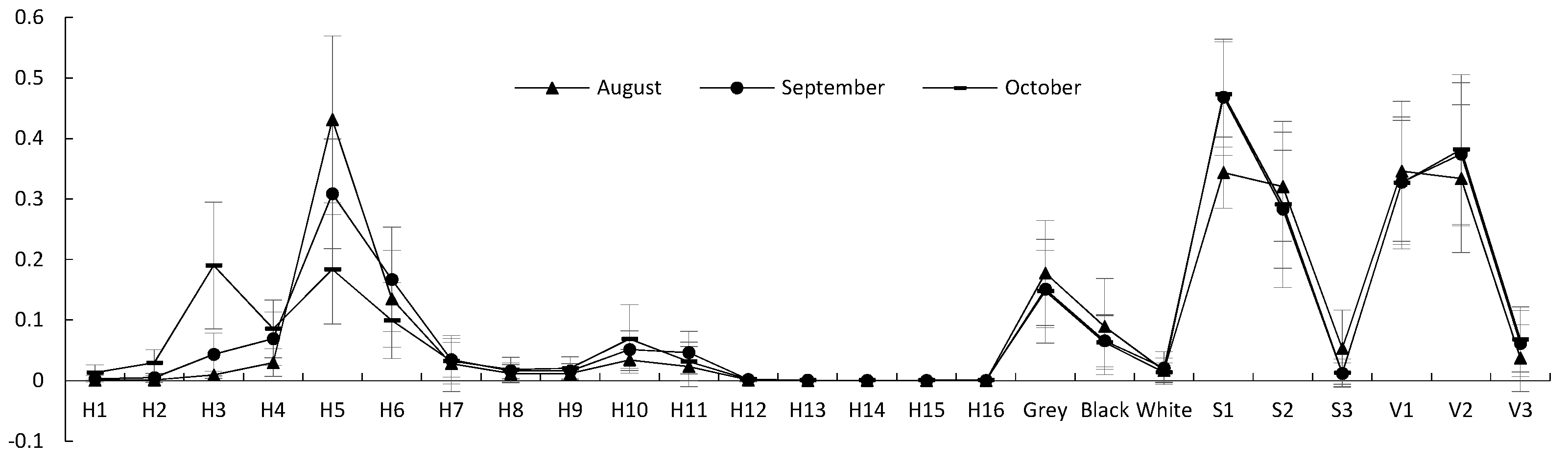
Figure 4 showed the proportion of color elements in autumn. From the hue, it is clear that there were significant quantities of green (H5, H6, H7, H8, H9) and yellow (H3, H4), whereas there was relatively little red (H1, H2) and blue-violet (H10, H11). There were almost no other colors. Colors of low saturation were higher than those of high saturation, and the rank order was S1 > S2 > S3. There were more medium-value colors than the high and low ones, sorted as follows: V2 > V1 > V3. In addition, the proportion of Black, White, and Grey was Grey > Black > White.

3.1.2. Comparison of Forest Color Element Variation over Time

With the change of autumn, colors in H1, H2, H3, H4, H8, H9, H10, H12, H13, H14, H15, and H16 increased gradually, but colors in H6, H7, and H11 increased at first and then decreased. H5 showed a decreasing trend (see Figure S5 for more details). One-way ANOVA indicated that the majority of differences in color elements over three months were significant (p < 0.05) or very significant (p < 0.01), except for colors in H7, H8, H9, H12, H13, and H14. In addition, the multiple comparisons suggested that there was no significant difference in H1, H2, H15, and H16 between August and September, although they were different in October. H4 in August differed in September and October. H5 had significant differences. H6 changed conspicuously between September and October, but these two months did not exhibit significant differences from August. H10 and H11 were similar to H6, but the months where significant differences existed were different, namely in August, October, and September (see Table S1 for more details). Significant differences in forest saturation and value over three months were tested (see Table S2 for more details). S1 and S2 showed significant differences. S1 increased gradually with time, but S3 was contrary to S1. This means that the forest’s saturation was diminishing in autumn in Jiuzhai Valley. From the percentage changes, Grey, Black, S2, and V1 decreased gradually, and in addition to White tending to decrease after the rising to a peak, other variables all increased. With the exception of S1 and S3, however, there were no obvious differences.

One-way ANOVA regarding the number of colors (NC) and maximum hue index (MHI) indicated that they were both very significant, showing considerable change (see Table S3 for more details). The three values of NC were 14.636, 19.88, and 22.292, exhibiting a significant increase. Moreover, the three in MHI were 0.453, 0.325, and 0.253, which decreased significantly.

3.1.3. Comparison of Forest Color Patch Variation over Different Months

The color diversity in patches (CD) and the color patch perimeter-area ratio (PARA) exhibited significant differences (

Table 3. Differences in forest color patches over three months.

Indicator	AP	BP	SP	NP	CD	ARP	PD	LPI	LSI
F	1.494	0.898	3.088	2.240	7.949	1.397	2.594	1.278	1.464
P	0.229	0.411	0.050	0.112	0.001	0.252	0.080	0.283	0.236
Indicator	PARA	CON	DIV	SPL	SHDI	SIEI	AI	PLA	COH
F	3.183	1.161	.892	0.805	0.387	1.592	1.570	1.326	0.770
P	0.046	0.317	0.413	0.450	0.680	0.209	0.213	0.270	0.466

Note: AP means proportion of coniferous forest; BP means broad-leaved forest proportion; SP means shrubwood proportion; NP means number of patches; CD means color diversity in patches; ARP means the mean area proportion of the color patch; PD means color patch density; LPI means largest color patch index; LSI means color landscape shape index; PARA means color patch perimeter-area ratio; CON means contagion of color patch; DIV means landscape division index of color; SPL means splitting index of color patch; SHDI means Shannon’s diversity index of color patch; SIEI means Simpson’s evenness index of color patch; AI means aggregation index of color patch; PLA means proportion of alike adjacencies of color patch; COH means color patch of cohesion index.

). Except for these two indicators, however, the others were not significant. The CD values over three months were 1.091, 1.778, and 2.083, and the PARA values were 125.839, 187.376, and 249.807. Thus, they both increased over time.

3.2. Relationship between Forest Color Characteristics and SEB Values

As explained above, lighting (i.e., the orientation of the mountain slope) and fallen leaves were the main environmental disturbances in the study. ANOVA indicated that the SBE values were very significant (p = 0.009; p = 0.001) when these two factors changed. Consequently, partial correlation analysis was performed to control the effect of non-color elements.

3.2.1. Relationship between Forest Color Elements and SBE Values

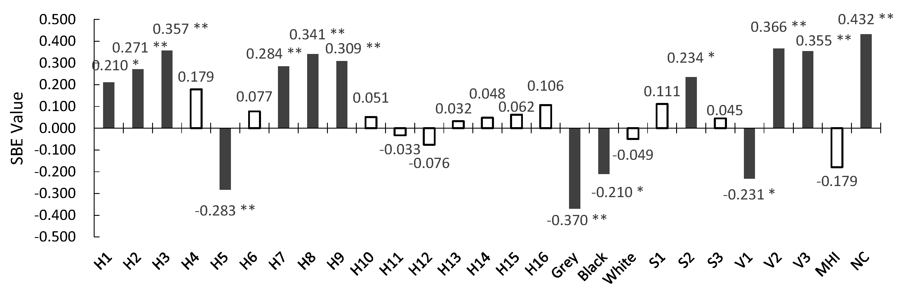
The correlations between H1, H2, H3, H5, H7, H8, H9, Grey, Black, S2, V1, V2, V3, and the SBE values were found to be significant or very significant, but other color elements were not significant (Figure 5). In this study, those parameters that have no significant correlation with SBE values were deleted. Among the preserved variables, some were positively correlated with SBE values. From large to small, they were ordered as follows: NC > V2 > H3 > V3 > H8 > H9 > H7 > H2 > S2 > H1. Some were negative correlations, which were ordered as follows: Grey > H5 > V1 > Black.

3.2.2. Relationship between Forest Color Patch Structures and SBE Values

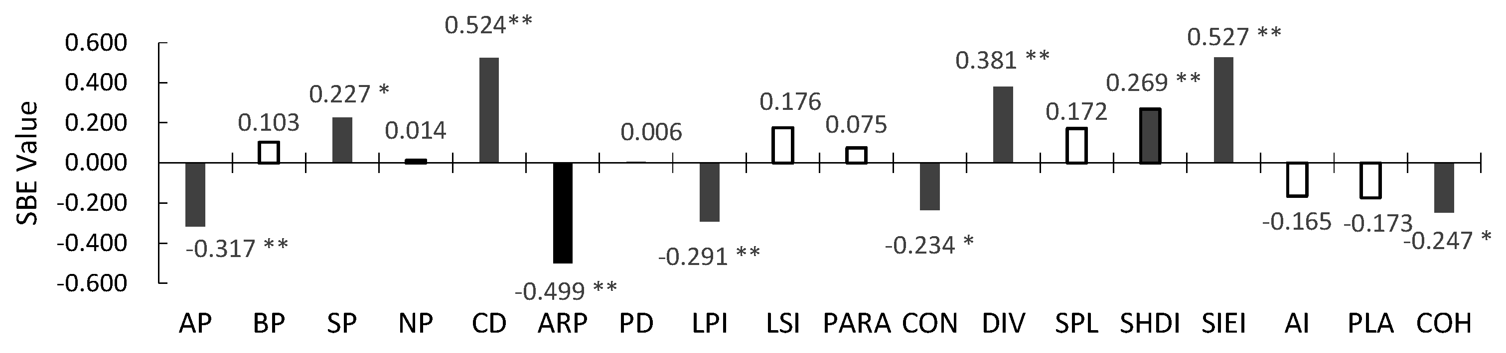
The parameters of shrubwood proportion (SP), color diversity in patches (CD), landscape division index of color (DIV), Shannon’s diversity index of color patch (SHDI), and Simpson’s evenness index of color patch (SIEI) showed significant or very significant positive correlations with the SBE values. According to the correlation coefficient from large to small, they were ordered as SIEI > CD > DIV > SHDI > SP. The indicators of the proportion of the coniferous forest (AP), mean area proportion of color patch (ARP), largest color patch index (LPI), contagion of color patch (CON), and color patch of cohesion index (COH) showed significant or very significant negative correlations with the SBE values. The correlation coefficient from large to small was as follows: ARP > AP > LPI > COH > CON (Figure 6).

3.3. Comprehensive Index Construction of Forest Colors

There were many indicators significantly correlated with SBE values. Therefore, in order to simplify research parameters, PCA was used to integrate indicators with a strong correlation together by controlling non-color elements. After transformation, the Kaiser–Meyer–Olkin (KMO) index was 0.624, showing that the variables were suitable for analysis. The accumulative contribution rates of the first six factors were 24.786%, 40.572%, 55.577%, 68.526%, 77.111%, and 83.266%. Therefore, these six factors could be used to explain all the variables.

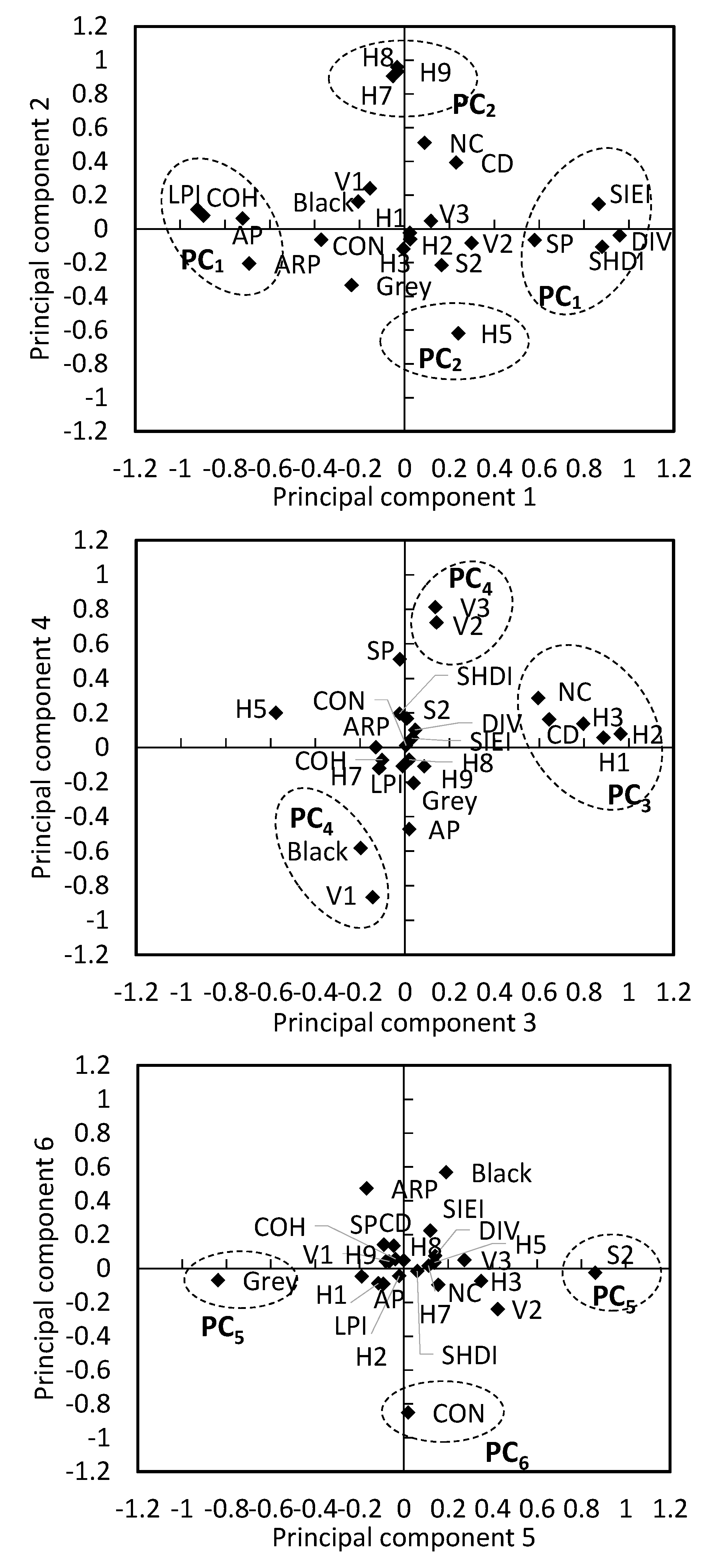
The results from the rotated component matrix are shown in Figure 7. PC₁ was strongly correlated with the landscape division index of color (DIV, 0.959), largest color patch index (LPI, −0.923), color patch of cohesion index (COH, −0.896), Shannon’s diversity index of color patch (SHDI, 0.881), Simpson’s evenness index of color patch (SIEI, 0865), shrubwood proportion (SP, 0.58), and the proportion of the coniferous forest (AP, −0.721). PC₁ reflected the broken and discrete degree of color patches. As such, it was named as the color patch fragmentation index. PC₂ was in close relation to H8 (0.96), H9 (0.933), H7 (0.906), and H5 (−0.618). These four indicators were all green. Hence, PC₂ was defined as the green leaves change index. PC₃ was strongly correlated with H2 (0.963), H1 (0.887), H3 (0.797), color diversity in patches (CD, 0.644), and the number of colors (NC, 0.595). These indicators changed significantly with autumn. Thus, PC₃ was defined as the yellow and red leaves change index. PC₄ was closely related to V1 (−0.866), V3 (0.813), V2 (0.734), and Black (−0.581), which presented color value differences. Thus, PC₄ was defined as the value index. The relationship between PC₅, S2 (0.863), and Grey (−0.838) was correlated. Thus, PC₅ was defined as the saturation index. PC₆ was in close relation to the contagion of color patch (CON, −0.851). Consequently, PC₆ was defined as the color patch contagion index.

After simplifying the factor count and calculating the weight of each variable in its factor, the equations were as follows (more details about the six simplified factors, significant correlation factors, and vegetative cover composition of the eight pictures in Figure 1 can be seen in Table S4):

$$\begin{gathered} P{C}_1=-0.073\times AP+0.049\times SP-0.147\times LPI+0.153\times DIV+0.139\times SHDI \\ +0.133\times SIEI-0.158\times COH-0.148\times ARP \end{gathered}$$

(11)

$$P{C}_2=-0.139\times H_5+0.282\times H_7+0.297\times H_8+0.283\times H_9$$

(12)

$$P{C}_3=0.243\times H_1+0.270\times H_2+0.230\times H_3+0.108\times NC+0.148\times CD$$

(13)

$$P{C}_4=-0.177\times BLACK-0.326\times V_1+0.188\times V_2+0.309\times V_3$$

(14)

$$P{C}_5=-0.472\times GREY+0.528\times S_2$$

(15)

$$P{C}_6=-CON$$

(16)

Further, Pearson correlation between simplified color factors and SBE values showed significant or very significant positive correlations. Therefore, the six simplified factors could explain the overall variables well, and correlations remained (

Table 4. Pearson correlation between simplified color factors and SBE values.

	SBE	PC1	PC2	PC3	PC4	PC5	PC6
SBE	1
PC1	0.462 **	1
PC2	0.281 *	−0.033	1
PC3	0.421 **	−0.860 **	0.080	1
PC4	0.376 **	0.043	−0.232 *	0.118	1
PC5	0.410 **	−0.073	0.023	0.101	0.349 **	1
PC6	0.247 *	0.991 **	−0.022	−0.863 **	0.013	−0.094	1

Note: ** denotes p < 0.01, * denotes p < 0.05.

).

3.4. Classification of the Forest Color Landscape in Jiuzhai Valley

Clustering analysis of the SBE value and six factors was performed to divide forest color sceneries into three categories (T₁, T₂, T₃) and six subtypes (T_1-1, T_1-2, T_1-3, T_2-1, T_2-2, T₃). T₁ contained three subtypes, T₂ contained two subtypes, and T₃ contained only one. From

Table 5. Differences of SBE values and color factors in six categories.

Indicator	T1				T2			T3
	Total	T1-1	T1-2	T1-3	Total	T2-1	T2-2	Total
SBE	36.21 ± 12.35 A	50.94 ± 6.59 a	32.95 ± 4.09b	20.18 ± 3.73 c	−10.17 ± 9.33 B	−1.87 ± 2.53 d	−18.47 ± 4.47 e	−41.63 ± 6.30 Cf
PC1	0.22 ± 0.57 A	0.19 ± 0.52 a	0.18 ± 0.54 a	0.37 ± 0.74 a	−0.87 ± 1.03 B	−0.78 ± 0.91 b	−0.95 ± 1.23 c	−1.57 ± 1.84 Bbc
PC2	0.04 ± 0.90 A	0.18 ± 1.14 a	−0.02 ± 0.75 a	−0.04 ± 0.84 a	−0.24 ± 0.85 A	0.01 ± 1.12 a	−0.49 ± 0.43 a	−0.68 ± 0.35 Aa
PC3	0.06 ± 0.69 A	0.45 ± 0.76 a	−0.20 ± 0.55 b	0.04 ± 0.66 ab	−0.27 ± 0.29 A	−0.16 ± 0.31 b	−0.38 ± 0.24 b	−0.61 ± 0.05 Ab
PC4	0.12 ± 0.87 A	0.47 ± 0.79 a	0.06 ± 0.85 ab	−0.30 ± 0.86 bc	−0.43 ± 0.64 B	−0.14 ± 0.80 abc	−0.73 ± 0.22 c	−0.83 ± 0.69 ABc
PC5	0.18 ± 0.77 A	0.50 ± 0.96 a	−0.07 ± 0.67 b	0.28 ± 0.41 ab	−0.75 ± 1.20 B	0.04 ± 0.84 ab	−1.54 ± 0.97 c	−0.70 ± 0.90ABbc
PC6	0.15 ± 0.55 A	0.10 ± 0.55 a	0.26 ± 0.57 a	−0.05 ± 0.47 ab	−0.95 ± 1.27 B	−0.90 ± 0.80 bc	−1.00 ± 1.70 c	0.42 ± 3.87 Aab

Note: Different letters indicate significant differences at the 0.05 level.

, SBE values decreased successively with T₁, T₂, and T₃. Therefore, the three categories of forests could be defined as the scenery superiority forest (T₁), scenery supplementary forest (T₂), and potential ascension forest (T₃).

Among the six values of the three categories, the color patch fragmentation index (PC₁), the green leaves change index (PC₂), the yellow and red leaves change index (PC₃), the value index (PC₄), and the saturation index (PC₅) decreased linearly with a decreasing SBE value. However, the color patch contagion index (PC₆) increased after the first decrease. Multiple comparisons showed that PC₂ and PC₃ were not significantly different among T₁, T₂, and T₃. With the exception of PC₂ and PC₃, other factors were significantly different between T₁ and T₂. SBE values and PC₆ were significantly different between T₂ and T₃, but other factors were not significantly different between these two categories. Multiple comparisons on six subtypes showed that PC₃ was not significantly different between T_1-1 and T_1-2, T_2-1, T_2-2. In other factors, the significance of difference in the subtypes was the same as that in the categories.

Differences in forest color variables in the six categories showed that H1, H2, H3, H7, H8, H9, V2, V3, number of colors (NC), shrubwood proportion (SP), color diversity in patches (CD), landscape division index of color (DIV), Shannon’s diversity index of color patch (SHDI), and Simpson’s evenness index of color patch (SIEI) decreased linearly. However, H5, Grey, Black, V1, proportion of coniferous forest (AP), largest color patch index (LPI), color patch of cohesion index (COH), and the mean area proportion of color patch (ARP) increased linearly. S2 increased after the first decrease, and the contagion of color patch (CON) was the opposite of S2, which first increased and then decreased (see Table S5 for more details).

Multiple comparisons showed that H1, H2, H3, H5, H7, H8, H9, Black, and V1 were not significantly different among T₁, T₂, and T₃, and that other variables were significantly different in T₁, T₂, T₃ or in T₁, T₂. Among the six subtypes, H1, H2, and H3 were significantly different between T_1-1 and the other five subtypes. Other variables were the same as the factors they belonged to. In general, the significant differences in forest color variables were basically the same as those in the principal factors simplified, which the variables belonged to. In addition, Black and V1 were not the only indicators composing the value index (PC₄). These were affected by V2 and V3 such that PC₄ showed significant differences.

After synthesizing the values distribution and performing multiple comparisons of principle factors and color variables, it was clear that the green leaves change index (PC₂) and the yellow and the red leaves change index (PC₃) had less influence on SBE beauty than the color patch fragmentation index (PC₁), the value index (PC₄), the saturation index (PC₅), and the color patch contagion index (PC₆).

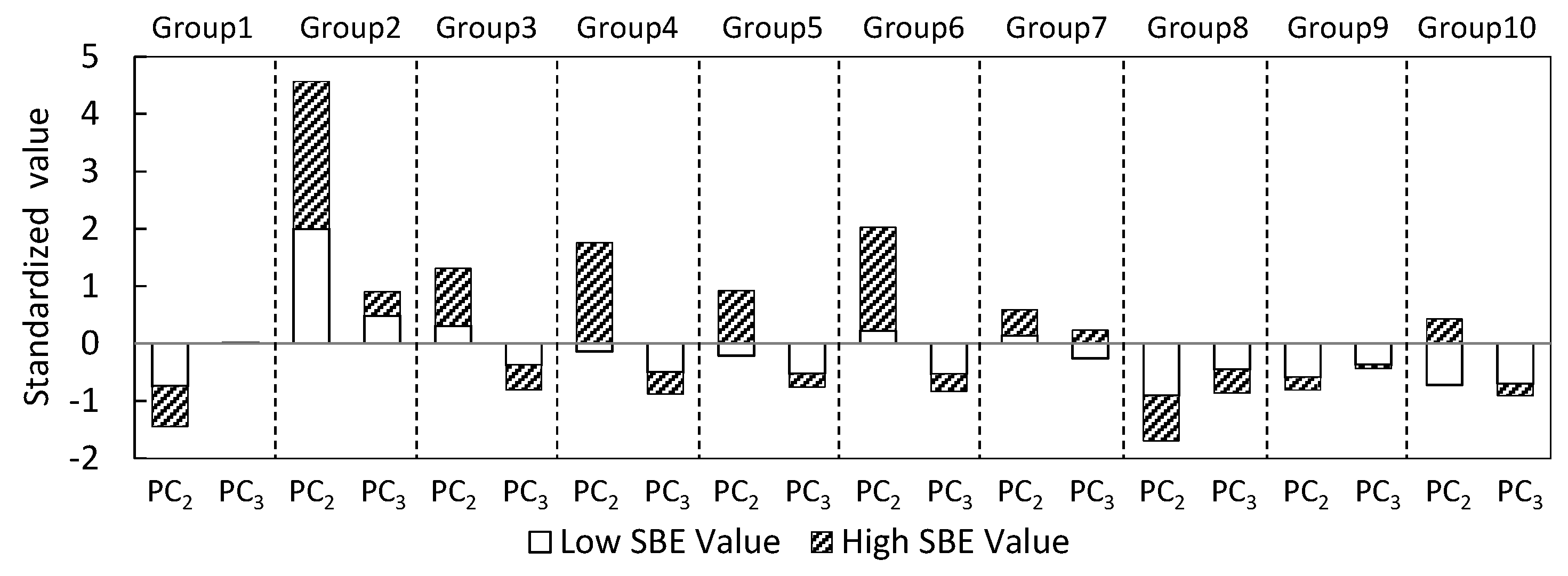
3.5. Variation Tendency between PC₂, PC₃, and SBE Values

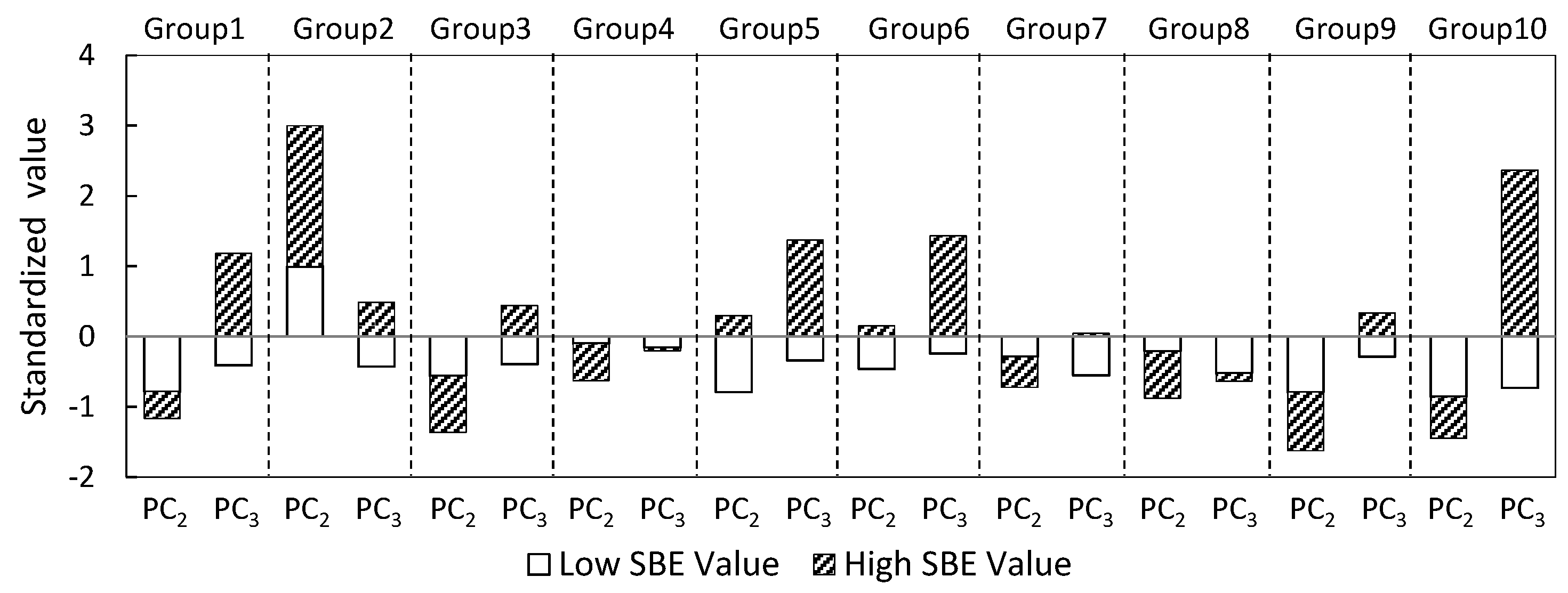
As explained above, when the color patch fragmentation index (PC₁), the value index (PC₄), the saturation index (PC₅), and the color patch contagion index (PC₆) were significantly different, the green leaves change index (PC₂) and the yellow and red leaves change index (PC₃) were not significantly different from the SBE value. At the same time, there were no significant differences in some indicators of the PC₄, so PC₁, PC₅, and PC₆ were the main factors used to analyze the variation of PC₂ and PC₃, when SBE values were different. Two cases were included.

One case involved pictures taken from the same sample spots in different months. These were almost the same index as PC₁ and PC₆, when PC₂ and PC₃ were significantly different. We selected ten groups of pictures randomly. Each group contained two pictures taken in different months, where the colors were significantly different. Varying features of PC₂ and PC₃ in each group were found: in all groups, images with higher SBE values showed an increase in their PC₃ (Figure 8). PC₂ in Groups 3, 4, 7, 8, and 9 was lower when the SBE value was higher, but in other groups, it was higher. Thus, there was no evident regularity found suggesting that PC₂ was related to SBE values in Case 1.

The second case involved pictures taken in different sample spots, in which PC₁, PC₅, and PC₆ were similar. We selected ten groups of pictures randomly, as with Case 1. The results showed that PC₂ was higher as the SBE value increased, while PC₃ was almost unchanged in Groups 1, 2, 4, and 6 (Figure 9). In other groups, PC₂ and PC₃ were both higher with a higher SBE value.

4. Discussion

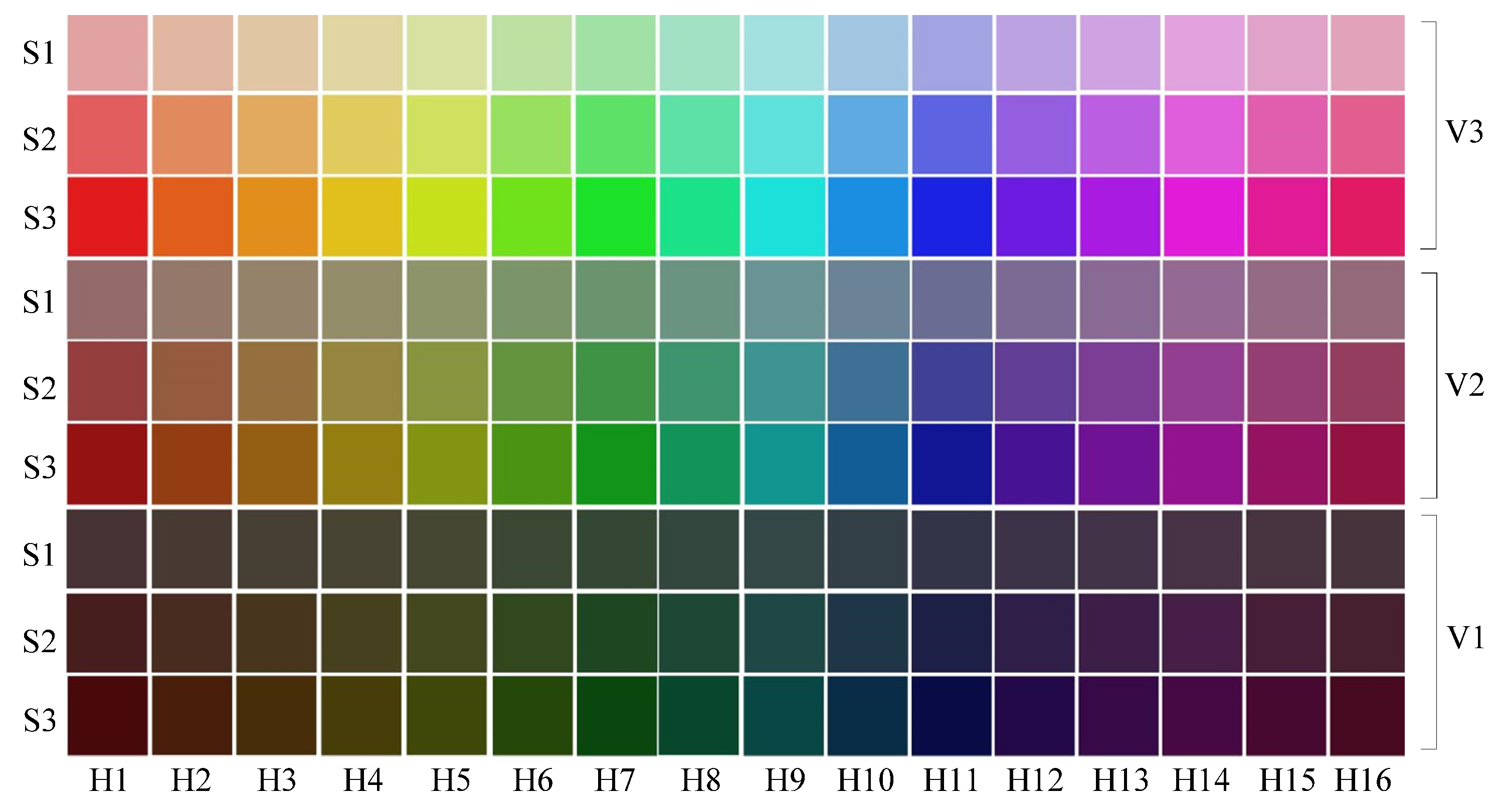
The correlations between forest colors and forest scenic beauty have been previously confirmed [23], but the excavation of color indicators mostly remained at the qualitative-oriented level. This paper found that self-programming had a certain advantage in the quantitative analysis of forest color pictures, which can be used to choose the color indicators according to the research content and requirements. In this paper, 16 types of hue, three types of saturation, three valuation types, and Black, White, and Grey were selected to classify and summarize the colors of Jiuzhai Valley forests. In future research, it will be possible to refine the colors within the color gamut of tree species according to research priorities and needs. These research needs might include studying the color variation of a tree species. Indeed, each hue can be separated into nine or more independent colors.

In general, the hue of the Jiuzhai Valley forest in autumn was mainly yellow (H3, H4) and green (H5, H6), and the proportion of red (H1, H2) was very small. The main factor was the saturation S1. In terms of value, V2 accounted for the most. As the months changed, the colors of red (H1, H2) and yellow (H3, H4) increased significantly. There was an increase in yellow, and the change in green was not uniform. Meanwhile, the saturation decreased and the value increased. This change was consistent with the Jiuzhai Valley’s plant species and the characteristics of seasonal change. The phytocoenosium of Jiuzhai Valley is mainly composed of Betula Linn., Alibes Mill., Quercus Linn., Picea wilsonii Mast., Pinus tabuliformis Carr., and Picea Dietr. The forest with a large area of evergreen coniferous trees had lower color saturation and value than the deciduous broad-leaved forest [32]. The leaves of deciduous broad-leaved species (Betula platyphylla Suk., Betula albosinensis Burk., etc.) in autumn were mainly yellow, which was also the main reason for the higher proportion of yellow. Sun also verified the tendencies between plant type and color change [13]. Moreover, there were a variety of plants in Jiuzhai Valley with red leaves in autumn—e.g., Cotinus szechuanensis A. Penzes, Acer davidii Franch., Sorbus hupehensis Schneid., Berberis veitchii Schneid., Cotoneaster adpressus Bois, etc. However, the proportion of red remained relatively small. On the one hand, this might be because of the small distribution range of red-leaf plants in some survey plots. On the other hand, this might be due to the geographical features of Jiuzhai Valley. As previously demonstrated, the prevalence of red-colored plants is closely related to climate [33]. However, the elevation of Jiuzhai Valley is relatively high, and the weather is commonly windy and rainy. During the survey, many plants began to defoliate before the frost, resulting in a lower proportion of red-colored plants. Despite this, the number of colors (NC) and the main hue index (MHI) significantly increased and decreased respectively with time. Both were affected by the discoloration of plant leaves.

There were no significant changes in color patch indices in different months, except for the color diversity in patches (CD) and the color patch perimeter-area ratio (PARA), both of which increased over time. This suggests that the distribution pattern and the spatial relationship between color patches do not change significantly over time, except in terms of the number of mixed colors in the color patches and the shape of some patches. Thus, in autumn, the color change in Jiuzhai Valley is mainly reflected in the change of color composition elements. The color patches layout exhibited almost no significant change. That is mainly because the composition of plant communities is the main factor that determines the layout of the color patches [30], which is not affected by changes in color.

The different orientation of the sample plot would lead to discrepancies in the shooting light, which was an environmental interference factor in this study. Moreover, fallen leaves were another problem. We showed that both of these factors had a significant influence on the SBE value. Therefore, those two indicators were used as control variables for the partial correlation analysis. The results showed that the number of colors (NC), V2, H3, V3, H8, H9, H7, H2, S2, and H1 had positive correlations with the SBE values in the order from large to small, and Grey, H5, V1, and Black had negative correlations with the SBE values in the order of closest to farthest. This indicates that colorful leaves, the green color, higher value, and saturation were closely related to the SBE values, while the lower value and saturation exhibited the opposite effect. The correlation between the color patch index and the SBE values showed that when the values of the shrubwood proportion (SP), the color diversity in patches (CD), the landscape division index of color (DIV), and the Shannon’s diversity index of color patch (SHDI) were higher, they were closely correlated with high SBE values. However, when the proportion of coniferous forest (AP), the mean area proportion of color patch (ARP), the largest color patch index (LPI), and the color patch of cohesion index (COH) were higher, they were closely correlated with a low SBE value. This is consistent with the results obtained by Mao in the study of in-forest landscapes [30]. According to species composition, it is obvious that sceneries are in low beauty values when they are comprised by some purely (or mostly) coniferous trees of lower saturation and lightness with discoloration in autumn, such as Picea wilsonii Mast., Pinus tabuliformis Carri, Abies ernestii Rehd., Pinus armandii Franch., etc. 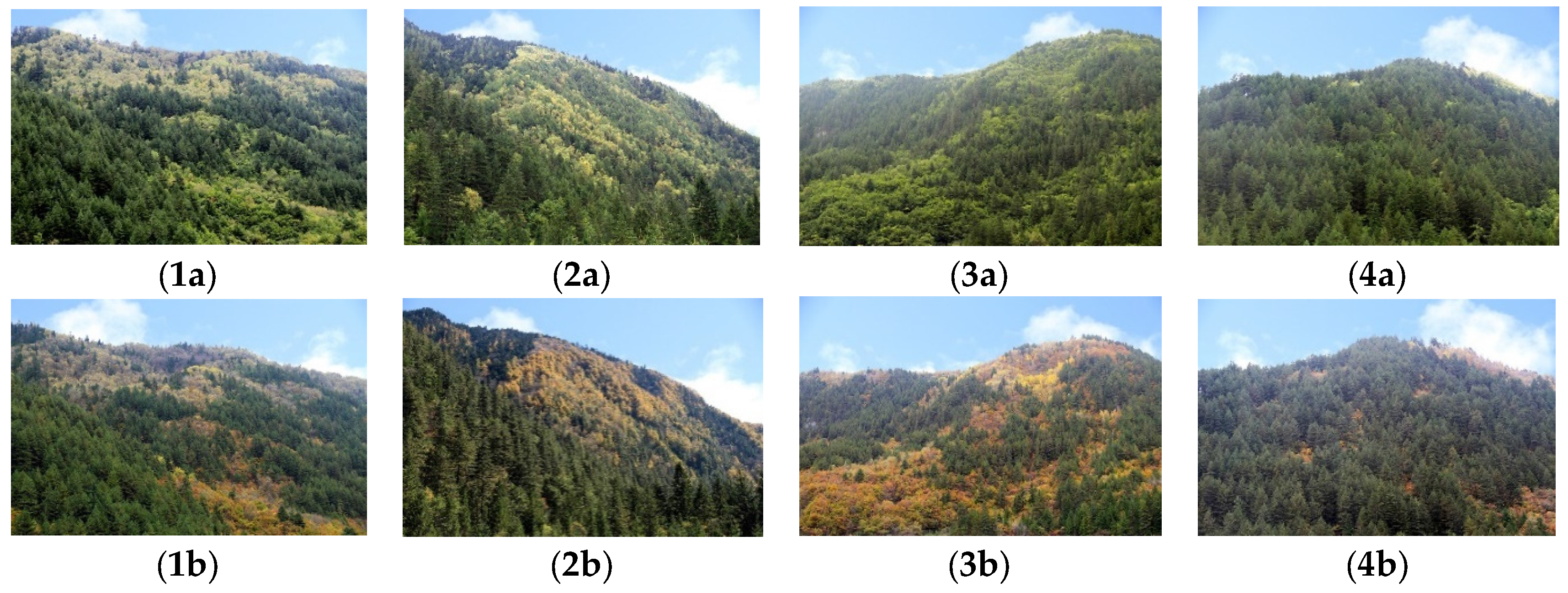Furthermore, it turns to high value when they consist of a large amount of plants with color changing in autumn, and higher lightness and saturation, such as Populus davidiana Dode, Quercus wutaishanica Mayr, Betula platyphylla Suk., Betula albosinensis Burk., Fraxinus chinensis Roxb., etc., and added to mixed forests that are mainly coniferous forests. It can also be seen through Figure 1. In picture 2a, there are certain portions of Quercus wutaishanica Mayr, Betula platyphylla Suk., Betula albosinensis Burk., etc. in which some sceneries of more color patches are formed, with rather dispersed distribution together with Abies ernestii Rehd. Furthermore, in autumn, the leaves are colorful with higher saturation and lightness. Furthermore, in picture 2d, it is Abies fabri forest which contains less fragmentations with an integral and big patch, and the forest’s saturation and lightness are also low with no colorful leaves. Therefore, the scenic beauty value of image 2a is obviously higher than that of image 2d.

The forest color elements and the color patch distribution indicators can accurately reflect color differences in the Jiuzhai Valley forest. However, there were too many indicators, and these were not completely independent. PCA can represent all the indicators with fewer factors, and this was practical [24]. In this paper, we used six factors to explain and to screen the correlated variables. Meanwhile, we combined the SBE values for clustering analysis. From the results, we observed the change between the principal component factors among different categories and the SBE values. First, when the averaged value of the color patch fragmentation index (PC₁), the value index (PC₄), and the saturation index (PC₅) were 0.22, 0.12, and 0.5 (after normalization), the SBE values were significantly high and decreased with the reduction of these three factors. This suggested that forests with color patches that were more scattered and divided, and that were composed of many species of higher value and saturation, had a relatively higher SBE value. Second, when the average color patch contagion index (PC₆) was 0.15, the SBE was the highest, and the SBE value was relatively low when the PC₆ was larger or smaller. In addition, in the forest color landscape categories with multiple comparisons, the following results were obtained. Some indices, such as the yellow and red leaves change index (PC₃), showed significant differences in a certain subtype (T_1-1, T_1-2, T_1-3). Moreover, there were corresponding color variables (H1, H2, H3), which were also significantly different for this subtype, but there was no obvious difference in the larger categories (viz., T₁, T₂, and T₃). This fact might be explained by the large number of samples included in this large category, because this results in the fluctuation of this index among the samples. For example, two images with the same PC₃ generated totally different SBE values because of the discrepancy of indicators, such as the proportion of coniferous forest (AP) and the landscape division index of color (DIV). As shown in picture 3b in Figure 1, the scenic beauty value is 53.91 which is the highest among the 8 pictures. The scenery is comprised of Abies ernestii Rehd., Pinus tabuliformis Carri., Populus davidiana Dode, Betula platyphylla Suk., Betula albosinensis Burk., Quercus wutaishanica Mayr, etc. The plant pieces are abundant, and the number of colors reaches 27 after quantification. These broad-leaved trees show higher brightness and saturation with red and yellow in autumn, thus values of PC₃, PC₄, PC₅ are higher; the color patches show much fragmentation with many divisions, thus PC₁ is higher; each type of color patch is in moderate connection, with medium size and distance from each other, therefore, PC₆ is in medium value.

The study of color-comprehensive factors and SBE values found that the green leaves change index (PC₂) and PC₃ had no apparent correlation with SBE values. However, according to the single index correlation analysis results, there was a significant correlation between PC₂ and PC₃ and the SBE values. The most likely reason for this was that PC₁, PC₄, PC₅, and PC₆ had a significant influence on the SBE values. Therefore, in this paper, by controlling PC₁, PC₅, and PC₆, we divided the images into two cases: same and similar values of the color patch index. We then performed random sampling for further analysis. In the pictures taken at the same plot in different months, such as images 1a and 1b, 2a and 2b, 3a and 3b, 4a and 4b in Figure 1, the results showed that pictures of higher PC₃ value had higher SBE values. In pictures with a similar color patch index and saturation index taken in different plots, such as images 1a and 2a in Figure 1, PC₂ and PC₃ both had a positive correlation with the SBE values, and PC₂ had a stronger influence than PC₃.

5. Conclusions

The color elements affecting the SBE values of Jiuzhai Valley were mainly the number of colors (NC), V2, H3, V3, H8, H9, H7, H2, S2, H1, Grey, H5, V1, and Black. These elements can be summarized as the green leaves change index (PC₂), the yellow and the red leaves change index (PC₃), the value index (PC₄), and the saturation index (PC₅). The color patches’ composition indicators affecting the SBE values in Jiuzhai Valley were the shrubwood proportion (SP), the proportion of coniferous forest (AP), the color diversity in patches (CD), the landscape division index of color (DIV), Shannon’s diversity index of color patch (SHDI), the mean area proportion of color patch (ARP), the largest color patch index (LPI), and the color patch of cohesion index (COH). Among these, CD can be classified into PC₃, and the remaining indices can be summarized as the color patch fragmentation index (PC₁) and the color patch contagion index (PC₆). PC₂, PC₃, PC₄, and PC₅ were significantly correlated with the change of time. Furthermore, PC₁ and PC₆ were mainly influenced by the community structure, regardless of the change in time. PC₁, PC₄, PC₅, and PC₆ contributed the most to the SBE values. When the first three had higher values, the SBE value was also higher. However, PC₆ was larger or smaller when the SBE values decreased. On the one hand, by controlling the ranges of those four factors, we found that in pictures with almost the same controlled index taken in the same plots at different times, the simultaneous change relationship between PC₃ and the SBE values stood out. The SBE values were relatively high when PC₃ was relatively large. On the other hand, in pictures with a similarly controlled index taken in different plots, the contribution of PC₂ was more significant, and when PC₂ was larger, the SBE values were higher as well.

In the mingled forests composed of evergreen coniferous forests and defoliated broad-leaved forests, under the premise of forest management, modifying and improving colors of forest sceneries can be an effective way of increasing their beauty. (1) In pure stands of evergreen coniferous ones, increasing the autumn colors of broadleaf trees should be given priority, such as Acer Linn., Betula platyphylla Suk., and Betula albosinensis Burk., so as to improve forests’ beauty in autumn. (2) In pure or mixed stands of evergreen coniferous ones, increasing broad-leaved trees and shrubs with higher brightness and saturation, and greener colors such as Populus davidiana Dode, and Quercus wutaishanica Mayr, will help to raise the degree of forest sceneries even in a season with pure green leaves. (3) It is obvious that the mixed forests with coniferous and broad-leaved trees are the most abundant color diversity, so beauty values are higher than that of pure forests. Therefore, to consider management methods of creating appropriate mixed forests is to enhance the beauty of forests. (4) In terms of mixed landscapes, selecting 1–3 types of coniferous forests and 2–4 species of deciduous trees can create a beautiful landscape, if more focus is directed at maitaining the fragmented color patches, balancing the patch size (which should not be too big or small), and moderating the distance among the same color patches (which should beneither too close nor too far).

It is worth emphasizing that the conclusions drawn from the tendencies of the color comprehensive index and the SBE values were based on autumn landscape conditions and the particular color characteristics of Jiuzhai Valley forests over the course of three months. Owing to the limitations in vegetation type in the mountainous region along with environmental factors, it is possible that there were non-linear variations from some excluded values apart from the linear relationship described in this paper. Therefore, in order to construct a scenic beauty prediction model under the influence of the forest color elements and patch characteristics, we need to carry out more controlled experiments in the future.