Estimating Large Area Forest Carbon Stocks—A Pragmatic Design Based Strategy

Abstract

Reducing uncertainty in forest carbon estimates at local and regional scales has become increasingly important due to the centrality of the terrestrial carbon cycle in issues of climate change. In Victoria, Australia, public natural forests extend over 7.2 M ha and constitute a significant and important carbon stock. Recently, a wide range of approaches to estimate carbon stocks within these forests have been developed and applied. However, there are a number of data and estimation limitations associated with these studies. In response, over the last five years, the State of Victoria has implemented a pragmatic plot-based design consisting of pre-stratified permanent observational units located on a state-wide grid. Using the ground sampling grid, we estimated aboveground and belowground carbon stocks (including soil to 0.3 m depth) in both National Parks and State Forests, across a wide range of bioregions. Estimates of carbon stocks and associated uncertainty were conducted using simple design based estimators. We detected significantly more carbon in total aboveground and belowground components in State Forests (408.9 t ha⁻¹, 95% confidence interval 388.8–428.9 t ha⁻¹) than National Parks (267.6 t ha⁻¹, 251.9–283.3 t ha⁻¹). We were also able to estimate forest carbon stocks (and associated uncertainty) for 21 strata that represent all of Victoria’s bioregions and public tenures. It is anticipated that the lessons learnt from this study may support the discussion on planning and implementing low cost large area forest carbon stock sampling in other jurisdictions.

1. Introduction

Natural forests play a crucial role in the global carbon cycle; as such, maintaining and building natural forest carbon is central to mitigating carbon emissions to the atmosphere from the biosphere. Developing and implementing transparent and accurate methods to estimate natural forests’ carbon stocks and changes is challenging because of the variability at a regional scale, coupled with limited empirical forest biomass and soil carbon observations.

In Victoria, Australia, public natural forests extend over 7.2 M ha [1] and constitute a significant and important carbon stock that is subject to change through altered wildland fire regimes, and forest management activities including timber extraction, ecological thinning, and prescribed fire [2]. As a consequence, a wide range of approaches to estimate forest carbon stocks within these forests have been developed and applied [3,4,5,6,7,8,9,10,11,12,13,14].Unfortunately, there are a number of data and estimation limitations associated with these studies: (a) no estimation of uncertainty [3,4,6,7,8,12,13,14]; (b) field data have not been collected in a statistically defensible manner for design based estimation [3,6,8,9,10,12,14,15]; (c) bias assessment for the model-based estimation is missing and/or modelled predictions without independent ground plot observations [4,5,8,11,13]; (d) data and/or models have limited coverage of population [3,8,10,11,12,15]; (e) data excludes some carbon pools such as coarse woody debris and litter [3,6,13]; (f) data excludes some or all of understorey life forms [3,6,13]; (g) ground plot data have inconsistent standards between measurements [8,11,13].

In response to this situation, the Victorian Department of Environment, Land, Water and Planning has implemented the Victorian Forest Monitoring Program (VFMP) [16]. The VFMP is designed to overcome many of these limitations and, in addition, to meet the requirements for state assessment mandated by state and national reporting legislation and agreements. A primary focus of the VFMP is to address key knowledge gaps about carbon stocks in Victoria’s public forests, in particular to provide statistically defensible estimates utilising physical plot measurements for a range of large area strata. The VFMP is a pragmatic plot-based design consisting of permanent observational units located on a state-wide grid. Ground plots measurements are taken on large trees, small trees, herbs and shrubs, and down woody debris at the sample point. Soil and site descriptions are also recorded.

At the start of the development of the VFMP, there was no formal, ongoing strategic forest inventory that completely covered the total Victorian public forest area to provide the data required to meet statutory and national reporting requirements [16]. Through the development of the VFMP, Victoria has formally defined its public forests as having the ability to attain at least 2 m in height in situ with at least 20% canopy cover on a minimum area of 0.5 ha. Urban trees, shelterbelts, orchards, and horticultural trees are not included in the forest definition.

Five carbon pools are reported for natural forests within the VFMP:

(i)

aboveground live biomass, living stems, branches, foliage;

(ii)

belowground live biomass, living roots;

(iii)

dead wood not contained in the litter, either standing, lying on the ground, or in the soil;

(iv)

litter, fine litter, fumic, and humic layers; and

(v)

soil organic carbon to a specified depth of 0.3 m.

The belowground live biomass is currently estimated using root:shoot ratios. To estimate carbon stocks per hectare in the other four pools, trees and stand variables are measured within ground plots. The data are processed using a standardised reporting tool that calls a suite of customised scripts that query the quality assured VFMP mensuration database.

The first measurement of permanent sample plots on the state-wide grid was carried out during the annual measurement seasons between 2010 and 2015 with the objective of estimating per hectare carbon stocks as of 1 January 2013. Future re-measurements of the permanent sample plots are scheduled for 2016–2020 and will provide direct estimates of carbon sequestration.

This paper describes the field protocols, the carbon models, and the methods of obtaining forest carbon stocks using the VFMP. It presents estimates of per hectare carbon stocks as of 1 January 2013 for Victoria’s public forests for a range of large area reporting strata. It is anticipated that the lessons learnt from this study may support the discussion on planning and implementing low cost large area forest carbon stock sampling in other jurisdictions.

2. Materials and Methods

2.1. Study Area

The study area comprises approximately 7.2 million hectares of public land forests and parks tenure (hereafter, referred to as public land forests) in the state of Victoria, in southeast Australia. This area includes 4 million ha of national parks and conservation reserves, managed primarily for ecosystem and biodiversity protection, tourism, and recreation. The remaining 3.2 million ha are multiple-use state forest tenure, which include the provision of timber and non-timber forest products. Bounding extents of Victoria are north 141°47′36″ E 33°58′54″ S, east 149°58′36″ E 37°30′20″ S, south 146°17′13″ E 39°9′33″ S, and west 140°57′29″ E 34°28′23″ S.

Public land forests extend to all parts of the state and range from low multi-stemmed Mallee woodland across flat and gently undulating topography in the Northwest and Box-Ironbark forests, characterised by sparse to dense canopies of box, ironbark, and gum-barked eucalypts up to 25 m tall, on flat to undulating landscapes on rocky, auriferous soils across central Victoria. Highly variable medium and tall canopy damp sclerophyll forests are widespread across the study area, and are found on a range of loamy, clay-loam, and sandy-loam soils. Tall (up to and above 75 m) wet sclerophyll forests are found mostly in the eastern part of the study area on deep loamy soils at higher elevations. Dry sclerophyll forests are prevalent throughout the east, central, and southwest parts of the study area on clay-loam, sandy-loam, and shallow rocky soils of exposed hillsides, with canopies typically less than 25 m tall, with crooked, spreading trees [17].

The study area is characterised by a range of different climate zones and diverse topography. The northwest region experiences semi-arid conditions, with low median annual rainfall (less than 250 mm in parts), with coastal areas experiencing a cooler temperate climate. Dry inland plains dominate much of the central and western parts of the state. The Victorian Alps—part of the Australian Great Dividing Range mountain system—extend east-west from the centre of the study area, with elevations up to 2000 m. The Victorian Alps experience the lowest average temperatures and highest precipitation (greater than 1400 mm yr⁻¹) in the study area. This variety of climate and topography is reflected in the variation in forest types and structure across the study area.

2.2. Sampling Design

The guiding principle in developing the sampling design was that data resulting from the VFMP must be consistent: the same attributes must be measured over space and time, using the same standards, in a statistically defensible manner, at an acceptable level of precision. A supporting principle was the sampling design should be pragmatic and easy for practitioners to understand and use.

The sampling design has the following main elements:

(i)

target population is public land estate of Victoria;

(ii)

two-way stratification of bioregions and tenure, with varying sampling intensity among strata, so that each stratum is adequately sampled for statistical reliability;

(iii)

plot design having multiple field components; and

(iv)

stratified random sampling estimators.

Each component of the plot sampling design is explained in more detail below.

2.2.1. Target Population

The target population is the public land estate of Victoria. The target population is assumed to consist of an infinite number of points within the public land estate. The Victorian Public Land Management Classification system was used to delineate the public land estate [18].

2.2.2. Stratification and Sampling Density

The target population was stratified with respect to two factors, bioregion and tenure. Within each stratum, sample units were placed at the intersections of a grid (which utilised the VicGrid coordinate system [19]) whose spacing varied between 2 km and 20 km and was selected to produce a per stratum sample size of approximately 30 samples. The target within-stratum sample size of 30 samples was based on the assumption of a coefficient of variation for quantitative trait values (e.g., biomass) of at least 70% and a ‘desired’ (stratum level) target precision (standard error) of at most 12.5%. This resulted in 786 samples being selected for measurement.

2.2.3. Field Procedures

Field protocols for the selected sample location are described in detail [20]. The plot measurements are conducted on a range of inventory features located at the sample location:

• a 15 m radius plot around the sample location where a range of physical and biotic characteristics are assessed, including slope, aspect, topographic position, surface water, and disturbance agents;
• a 0.04 ha circular plot where all large trees (>10 cm in diameter) are assessed for: species, diameter at breast height over bark (dbhob), tree status, decay class, crown class. Additional measurements such as tree height, canopy cover, canopy health (discoloration, dieback, foliage density, epicormic growth, crown clumping) are made on a subset of these trees. Coarse woody debris (CWD), stumps and slash piles are also assessed across this plot;
• a 0.005 ha circular plot where all small trees (<10 cm in diameter) are assessed for species, frequency, and height;
• twelve 1 m² vegetation quadrats where a range of understory vegetation and groundcover parameters are assessed. These include frequency, cover and height of understorey species, total projected foliage cover, woody species cover, and percentage ground cover;
• on a subset of sampling points—four 0.25 m² soil quadrats where a range of soil and surface litter samples are taken for laboratory analysis. Analyses include humus (structure, litter, type); and
• on a subset of sampling points—a 1-m soil pit where soil profile observations are conducted in a representative part of the plot. Undisturbed soil vertical core sampling at 0–10, 10–20, and 20–30 cm depths from the pit profile wall for C and bulk density.

2.2.4. Sampling Estimators

One of the drawbacks of using a systematic sampling approach is the absence of unbiased estimators of the variance of the population parameters. However, we claim that for our purposes the location of the intersects of the state-wide grid can be assumed to be random. As a consequence, we interpret the 786 samples as coming from a stratified random sample. Therefore, we followed others [21,22,23] in employing the classical estimation formulae for stratified random sampling. We understand that the above assumptions may violate some sampling principles, but we consider that the impacts are negligible in practice and are outweighed by the benefits of utilising a sampling design that is pragmatic and easy for practitioners to understand.

2.3. Estimates of Carbon Stocks per Hectare

The aboveground living biomass of large trees (≥10 cm dbhob) were estimated using a generic allometric model for sclerophyll forests [24]. The model was of the form:

$$ln\left({\widehat{AGB\_LT\_LIVE}}_i\right)=-2.3267+2.4855\times ln\left(DBHO{B}_i\right)$$

(1)

where AGB_LT_LIVE_i is the aboveground biomass of live large tree i. Although species-specific models were available for over 25 of the 132 tree species assessed, there was no significant difference between stratum means using the generic and the species specific models. For simplicity, the above single generic model was utilised.

Small trees (<10 cm dbhob) were counted but not measured, so an estimate for each of the live small trees was estimated using a generic model for small eucalypts [24], of the form:

$$ln\left({\widehat{AGB\_ST\_LIVE}}_i\right)=-1.0668+\left(2.88807\times ln\left(H\right)\right)$$

(2)

where AGB_ST_LIVE_i is the aboveground biomass for live small tree i and H is the tree height.

Estimates of standing dead wood mass for large trees were calculated by first estimating aboveground biomass as for living trees using the whole tree allometric model (Equation (1)), and then reducing the estimated biomass by the amount of biomass in leaves, twigs, and branches. The following predictive model for estimating branches, bark, and leaf biomass specifically for Victorian forests was utilised:

$$ln\left({\widehat{AGB\_BBLB}}_i\right)=-2.99+2.22\times ln\left(DBHO{B}_i\right))$$

(3)

where AGB_BBLB_i is the mass (kg) of of branches, bark, and leaf biomass for standing dead tree i. Therefore, estimates of standing dead wood mass for large trees were achieved as follows:

AGB_LT_DEAD_i = (AGB_LT_LIVE − AGB_BBLB_i) × DSM_i

(4)

where AGB_LT_DEAD_i is the mass of standing large tree dead tree i, and DSM_i is a decay stage multiplier for tree i. A sound decay stage (decay stage modifier of 0.8) is assumed for standing dead wood, as any further decay stage would cause collapse of the standing dead wood and addition to the fallen CWD pool.

Since we need predictions from Equations (1)–(3) in arithmetic units rather than logarithmic units, the best-fit models were back-transformed to their original form. Reverse transformation on an arithmetic scale produces a systematic underestimation of the dependent variable [25,26]. Several procedures for correcting bias in logarithmic regression estimates have been reported. In this study, the logarithmic bias correction term added to the intercept for these three equations before back-transformation was:

$$CF=SE{E}^2/2$$

(5)

where CF is the correction factor and SEE² is the standard error of the estimation [25,27]. Estimates of standing dead wood mass for small trees were calculated by estimating aboveground biomass as for living trees and assuming a sound decay stage (decay state modifier of 0.8) as follows:

AGB_ST_DEAD_i = AGB_ST_LIVE × DSM_i

(6)

CWD is defined as all fallen dead woody material (branches, stems, logs) that were not rooted in the soil and with minimum cross-sections of 10 cm. All CWD pieces in the large tree plot were measured for length, assigned to 10 cm diameter classes, and assigned to a decay class. Decay was classified using a three point system based on previous assessments of eucalypt CWD [28], as outlined in

Table 1. Decay level of classes for coarse woody debris.

Class	Description	Decay State Modifier (DSM)
Sound	Intact with little evidence of decay (essentially hard, solid wood). Logs generally circular in cross section, and can support their own weight. Leaves, twigs, and branches may still be present, and bark is generally intact.	0.8
Moderate	Some sections may be pulled away by hand. Bark has generally become detached, and branches have mostly fallen off. Logs still largely circular in cross section, but hollows are developing at ends and where branches have detached. Stumps beginning to hollow out at top. In wet forests, moss may exceed 50% cover on the wood.	0.65
Advanced	Mostly rotten and hollow, and although the outer ‘shell’ may sometimes appear solid the inner material is able to be crumbled in the hand. Log unable to support its own weight and has collapsed to be elliptical in cross section. Stumps mostly collapsed. Other plants may be growing on the decaying wood (in wetter forest types), and there may be high moss cover.	0.50

. The mass of individual CWD pieces were calculated with the following model:

$$\begin{array}{c}CW{D}_i=AW{D}_i\times DS{M}_i\times V_i,\\ V_i=A{M}_i\times L_i,\\ A{M}_i=\pi {\left[\frac{MS{D}_i}{2}\right]}^2\end{array}$$

(7)

where CWD_i is the mass for piece i, AWD_i is the average wood density of tree species in Victoria (0.75 g·cm⁻³, [3]), DSM_i is decay-stage multiplier for piece i, AM_i is the cross-sectional area of piece i (in cm², the mid-range of diameter in a CWD diameter class), L_i is the length in cm, and MSD_i is the mid-section diameter class.

Mass of individual stumps was calculated as the remaining cross-sectional volume multiplied by the average wood density of trees species in Victoria (0.75 g·cm⁻¹) by decay classes per stand type (as above) using the following model:

$$\begin{array}{c}AGB\_STUM{P}_i=AW{D}_i\times DS{M}_i\times V_i,\\ V_i=A{M}_i\times H_i,\\ A{M}_i=\pi {\left[\frac{TOP{D}_i}{2}\right]}^2\end{array}$$

(8)

where AGB_STUMP_i is the aboveground biomass for stump i, AWD_i is the average wood density of tree species in Victoria (0.75 g cm⁻³), and DSM_i is decay-stage multiplier for stump i, AM_i is the cross-sectional area of stump i (in cm²), H_i is the stump height in cm , and TOPD_i is the top diameter of the stump i in cm. Tree (live, dead), CWD, and stump biomass by components and size class were summed for each sample plot (i.e., using individual large tree/stump values and multiplying single small tree/stump estimates by counts), and then multiplied by 0.5 to convert mass to carbon content. These data were then converted to carbon (C) in Mg ha⁻¹ by dividing by the appropriate plot area, which was corrected for slope.

Litter biomass included dead plant material such as fruits, leaves, bark, and small branches (<2.5 cm). Samples were collected from 0.25 m² frames and were sieved to remove any soil, large rocks, and CWD ≥ 2.5 cm. Samples were air-dried then oven-dried (70 °C, 24 h) to a constant recorded mass. Mass for each sample was divided by the quadrat area and averaged across the four samples to give plot-level litter mass.

Total root biomass was estimated using root:shoot ratios of 0.44, 0.28, and 0.20 for stems with aboveground biomass of <50, 50–150, and >150 Mg ha⁻¹, respectively. The ratios were recommended for temperate eucalypt forest based on a comprehensive review of major terrestrial biomes [29]. Root:shoot ratios were multiplied by large and small tree stem carbon and summed to give plot-level tree root carbon.

Soil samples were air-dried at room temperature, weighed, and gently sieved to <2 mm to remove any coarse roots or rocks. A subsample was oven-dried (105 °C, 24 h) to correct for volumetric water content in the calculation of bulk density (corrected for volume of stones estimated using a specific density of 2.65 g·cm⁻³; [30]). A representative sub-sample of air-dried soil was sieved and finely ground (<0.5 mm) for analysis of total carbon by dry combustion using a LECO CHN 1000 Analyser (LECO Corp., St. Joseph, MI, USA). Sample soil carbon stocks were calculated as the product of carbon concentration, bulk density, and depth, and plot-level soil carbon stocks (Mg ha⁻¹) were the average of four samples per 0.1 m depth interval.

2.4. Statistical Analyses

The VFMP estimated the biomass of living trees (large and small trees), deadwood biomass (dead large trees, dead small dead trees, stumps, and CWD), litter biomass, root biomass, and soil carbon with their standard errors, at the state and stratum levels. The mean of each carbon pool ($y_{st}$) for the population was calculated using the following equation (see [21], Equation (5.1) on page 91):

$${\overline{y}}_{st}={\displaystyle \sum }_{h=1}^L{N}_h{\overline{y}}_h/N={\displaystyle \sum }_{h=1}^L{W}_h{\overline{y}}_h$$

(9)

where

• L is the number of stratum;
• $N_h$ is the total number of units in stratum z;
• $W_h=Nh/N$ is the stratum weight of stratum h;
• ${\overline{y}}_h$ is the sample mean of stratum h; and
• $N=N_1+N_2+\dots N_l$

The standard error of ${\overline{y}}_{st}$ was calculated using the following equation (see [31], p. 30):

$$s_{{\overline{y}}_{st}}=\sqrt{\frac{1}{N^2}{\displaystyle \sum }_{h=1}^L\left[\frac{N_h^2{s}_h^2}{n_h}\left(1-\frac{n_h}{N_h}\right)\right]}$$

(10)

where

• $n_h$ is the number of units in sample; and
• $s_h^2$ is sample variance of stratum h.

To convert from biomass (Mg ha⁻¹) to carbon (t ha⁻¹) a common proxy was utilised, based on the assumption that 50% of the biomass is carbon [32]. However, it is acknowledged that this relationship may not hold constant over different tree species [33,34,35,36]. It was assumed that there was no error in the root-shoot models used to estimate belowground biomass. The uncertainty associated with the sum of the five estimates (aboveground living biomass, aboveground deadwood biomass, litter biomass, belowground biomass, and soil carbon) was calculated as the quadratic sum of the errors associated with the individual estimates, according to the rules for computing the propagation of uncertainties through the calculation [37].

To analyse the variability in the C-stock in the five main C pools, across the altitude gradient, each sample plot was assigned an altitude class (seven classes, 250 m wide, starting at sea level).

The dataset was also used to investigate the relationships, at the plot level, between litter and soil C-stocks and quantitative site features, qualitative forest stand features, and quantitative tree variables. Litter and soil C-stocks were not normally distributed and data transformation did not normalise the distribution. For this reason, the correlation analysis was performed using the non-parametric Spearman correlation coefficient. The variables that were significantly correlated with litter C-stock or with soil c-stock were identified as potential explanatory variables for multivariate regression analyses. The purpose of the multivariate regressions was to test the potential to predict litter biomass and soil carbon from either commonly available VFMP inventory data, or easily collected data. Litter C-stock was added as an additional potential explanatory variable in the soil C-stock prediction because the two variables were slightly but significantly correlated. In the end, the potential quantitative explanatory variables used in the regression analysis were: for site features, elevation, aspect, slope, aboveground live biomass, and aboveground deadwood biomass (standing dead large tree, standing dead tree, stumps, slash, CWD). A stepwise multiple linear regression method was used alternatively to select the most significant variables (probability of F-to-enter = 0.05; probability of F-to-remove = 0.1). The conventional multivariate regression model can be expressed as follows:

$$\widehat{Y}=a_0+a_1{X}_1+\dots +a_i{X}_i$$

(11)

where

• $\widehat{Y}$ is the dependent parameter to be predicted;
• $a_0$ is the intercept;
• i is the number of independent variables;
• $a_{1\dots i}$ are the regression coefficients; and
• $X_{1\dots i}$ are values of independent variables,

In this study, $\widehat{Y}$ refers to the litter C-stock per hectare and soil C-stock per hectare, $X_{1\dots i}$ represent values for elevation, aspect, slope, aboveground live biomass carbon aboveground deadwood biomass carbon, and litter C-stock (in the case of the soil C-stock regression). Collinearity was diagnosed through the Variance Inflation Factor (VIF). Generally, if the VIF is less than 10, collinearity is not serious [4,35].

3. Results

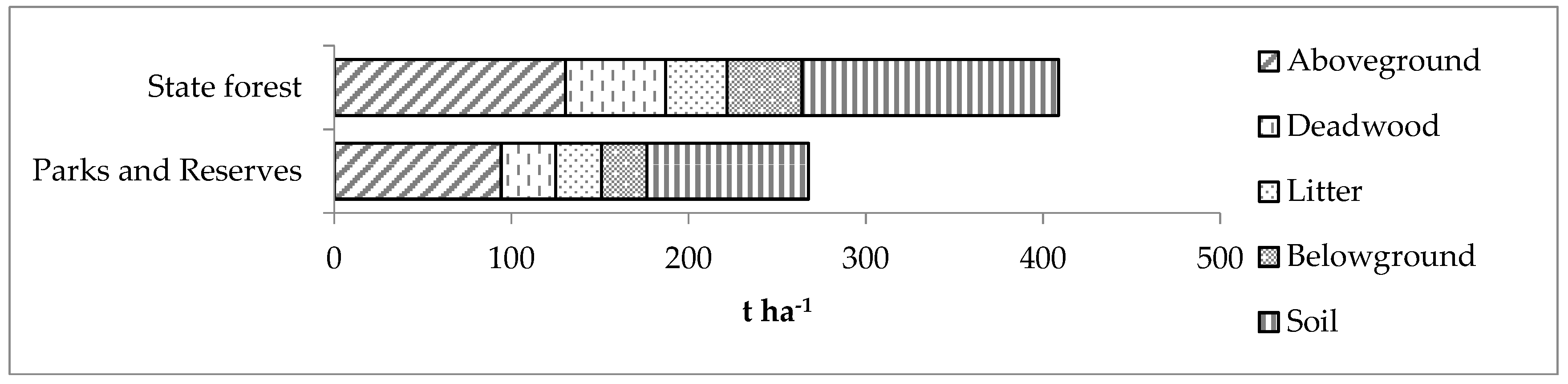
3.1. Carbon Stocks by Tenure Stratum

Table 2. Public land forest area within tenure categories and estimated carbon stock per hectare (with standard errors, S.E.) for different carbon pools.

Bioregion	Aboveground Living Biomass C-Stock (t ha−1)	S.E. (%)	Aboveground Deadwood Biomass C-Stock (t ha−1)	S.E. (%)	Litter C-Stock (t ha−1)	S.E. (%)	Belowground Biomass C-Stock (t ha−1)	S.E. (%)	Soil C-Stock (t ha−1)	S.E. (%)
Parks and Reserves	94.2	7.5	30.7	8.6	25.9	6.9	25.8	5.0	91.1	1.6
State forest	130.6	5.8	56.3	10.2	34.8	6.5	42.2	4.4	145.0	1.8

shows the estimates of C-stock per hectare, and related percent standard errors, for the aboveground living biomass, aboveground dead biomass, litter, belowground biomass, and soil by tenure category. Figure 1 shows the total carbon stock per hectare for the different tenure categories.

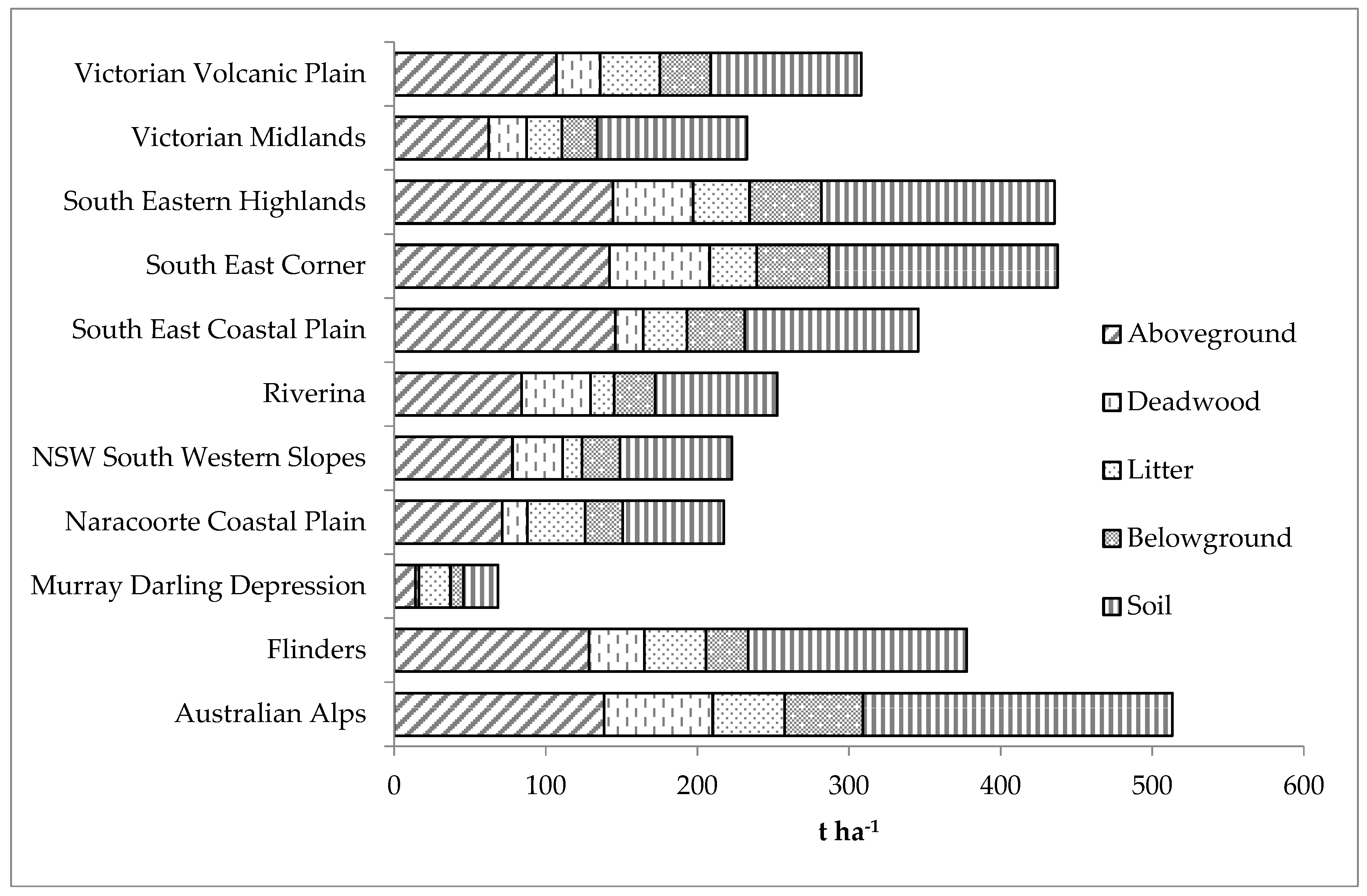
3.2. Carbon Stocks by Bioregion Stratum

Table 3. Public land forest area within bioregions and estimated carbon stock per hectare (with standard errors) for different carbon pools.

Bioregion	Aboveground Living Biomass C-Stock (t ha−1)	S.E. (%)	Aboveground Deadwood Biomass C-Stock (t ha−1)	S.E. (%)	Litter C-Stock (t ha−1)	S.E. (%)	Belowground Biomass C-Stock (t ha−1)	S.E. (%)	Soil C-Stock (t ha−1)	S.E. (%)
Australian Alps	138,4	10.1	71.7	9.5	47.3	7.5	51.6	5.7	204.2	3.4
Flinders	128.3	27.6	36.6	36.9	40.7	16.9	27.9	20.3	144.2	10.4
Murray Darling Depression	14.0	26.3	2.3	23.0	20.7	14.3	8.5	9.7	22.8	7.1
Naracoorte Coastal Plains	71.2	8.6	16.5	16.4	38.1	7.4	25.0	5.1	66.7	3.5
New South Western Slopes	78.0	9.0	33.0	8.8	12.7	8.3	25.2	5.6	73.8	3.6
Riverina	84.0	14.3	45.4	36.1	15.8	8.5	27.0	14.4	80.5	8.2
South East Coastal Plains	145.9	18.4	18.2	18.7	28.8	17.1	38.2	15.4	114.3	8.2
South East Corner	142.2	8.1	66.1	20.4	31.2	12.6	47.7	6.6	150.7	4.2
South East Highlands	144.2	8.0	52.9	10.4	37.3	9.0	47.3	6.1	153.9	3.2
Victorian Midlands	62.3	9.8	25.1	13.4	23.3	15.9	23.2	6.9	98.8	3.7
Victorian Volcanic Plain	107.00	19.2	29.0	26.2	39.3	22.5	33.4	17.2	99.5	7.9

shows the estimates of C-stock per hectare, and related percent standard errors, for the aboveground living biomass, aboveground dead biomass, litter, below ground biomass, and soil by bioregion category. Figure 2 shows the total carbon stock per hectare in the different bioregion categories.

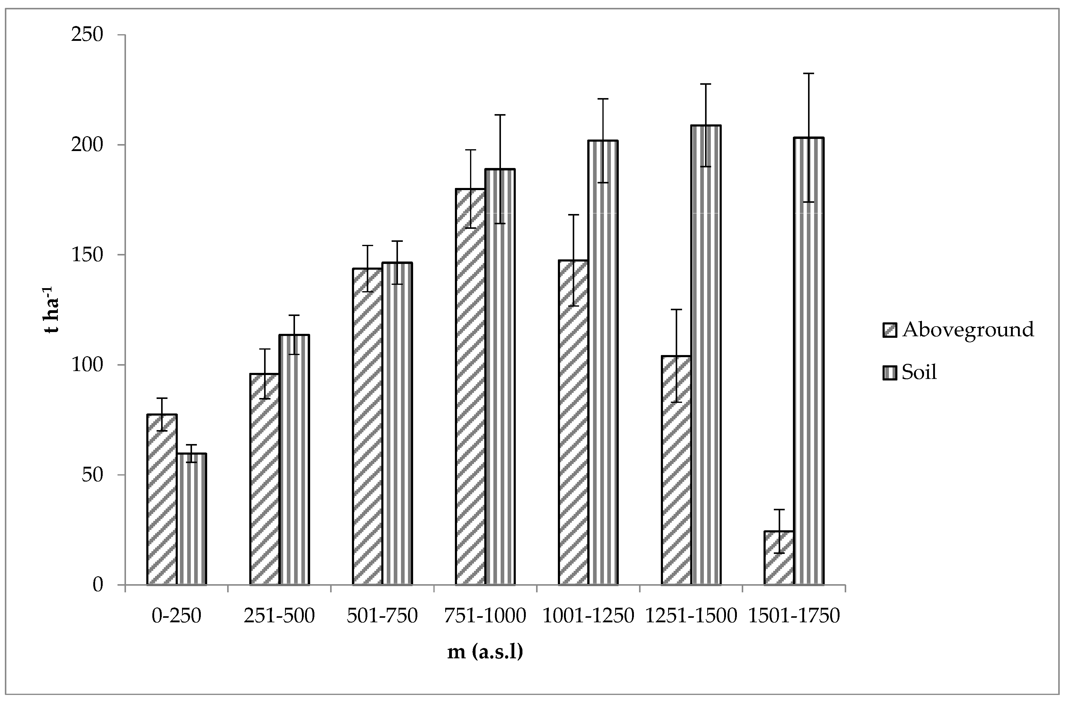
3.3. Relationship between Forest Carbon and Altitude

Table 4. Public land forest area within altitude classes (in metres above sea level (m a.s.l.)) and estimated C-stock per hectare (with standard errors) for different carbon pools.

Altitude Class (m a.s.l.)	Aboveground Living Biomass C-Stock (t ha−1)	S.E. (%)	Aboveground Deadwood Biomass C-Stock (t ha−1)	S.E. (%)	Litter C-Stock (t ha−1)	S.E. (%)	Belowground Biomass C-Stock (t ha−1)	S.E. (%)	Soil C-Stock (t ha−1)	S.E. (%)
0–250	77.4	9.6	33.5	14.1	40.8	6.7	20.6	6.8	59.7	6.6
251–500	95.9	11.8	65.2	10.9	35.9	9.4	34.1	8.1	113.6	7.8
501–750	143.7	7.3	68.4	8.4	68.7	8.4	46.2	5.5	146.4	6.7
751–1000	180.0	9.9	93.9	16.5	58.7	12.2	54.7	9.2	188.9	13.1
1001–1250	147.5	14.1	117.2	8.9	70.6	8.5	54.0	7.5	201.9	9.5
1251–1500	104.1	20.2	95.5	12.9	84.7	14.9	45.2	8.1	208.8	9.0
1501–1750	24.3	40.6	98.3	18.4	71.5	9.6	25.6	13.0	203.2	14.4

shows the estimates of C-stock per hectare, and related percent standard errors, for the aboveground living biomass, aboveground dead biomass, litter, belowground biomass, and soil by altitude classes. Figure 3 shows the aboveground living biomass carbon and soil carbon per hectare for the different altitude categories.

3.4. Relationship between Forest Carbon and Environmental Variables

Table 5. Correlation matrix. Spearman correlation coefficients (r) between litter C-stock and soil C-stock and some site/stand features at the stratum level.

Variable	Litter C-Stock (t ha−1)	Soil C-Stock (t ha−1)
Litter C-Stock (t ha−1)	1	0.21 ***
Soil C-Stock (t ha−1)	0.21 ***	1
Elevation (m a.s.l.)	0.11 **	0.50 ***
Slope (%)	0.04	0.42 ***
Aspect (degrees)	−0.02	−0.05
Aboveground living biomass C-stock (t ha−1)	0.10 *	0.37 ***
Aboveground deadwood biomass C-stock (t ha−1)	0.06	0.42 ***

* p-value < 0.05; ** p-value < 0.001; *** p-value < 0.0001.

shows the Spearman correlation coefficients between both litter C-stock and soil C-stock with different site/stand features as well as the other two carbon pools obtained in the field.

Stepwise multiple regression analysis was used to establish models to predict litter and soil C-stock, and the results are shown in

Table 6. Stepwise multiple regression results for litter C-stock and soil C-stock.

	Root Mean Squared Error	Adjusted R2	Model
Litter C-stock (t ha−1)	24.6	0.03	25.7 + 0.01 × elevation −0.03 × aboveground dead biomass C-stock
Soil C-stock (t ha−1)	54.4	0.32	66.5 + 0.08 × elevation + 0.13 × aboveground living biomass C-stock + 0.05 × aboveground dead biomass C-stock

. These models have a significance level of 0.01.

4. Discussion

4.1. Forest Carbon Stocks by Tenure

There are significant differences in total C-stock per hectare between Parks and Reserves and State forests (Table 2). It can be seen that the forests in Parks and Reserves have significantly lower carbon in all five pools. These differences are most likely due to a combination of environmental and historical land management practices, where the most productive land has been cleared for agriculture and of the remaining forested areas, the more productive forests have historically been managed for commercial forests (State forests). The investigation of these differences has been identified as an area of future research. This is the first Victorian forest land cover inventory which has attempted to provide statistical robust comparisons between land management tenures in terms of forest characteristics. Public land management agencies in Australia need to be aware of these differences in selecting appropriate systems and tools to support policy development.

4.2. Forest Carbon Stocks by Bioregion

There are considerable differences in total C-stock per hectare across the bioregions (range from 67.5 to 566.8 t ha⁻¹). This level of variation is consistent with previous field results [3,6]. It can be seen from both Table 3 and Figure 2 that the tall productive forests of the Great Dividing Range (Australian Alps, South East Coastal Plains, South East Corner) feature the larger levels of total-C-stock per hectare. Soil was the main carbon pool, followed by aboveground living biomass for all bioregions, except in New South Western Slopes and South East Coastal Plains, where this trend was reversed. As expected, the main component of the total-aboveground living biomass was standing large living trees (dbhob ≥ 10 cm), which contributed from 45.6% to 98.5% in each bioregion. The percentage of carbon stored in aboveground deadwood biomass in the bioregions ranged from 1.8% to 15.9%. Bioregions with the larger percentages of aboveground deadwood biomass tended to be regions with higher ratios of dead stems to all stems, often related to having a higher proportion of old growth forests and recent fire history. The presence of coarse woody debris was of only secondary importance in aboveground deadwood biomass. For the main carbon pools, soil is less variable between the bioregion categories than other pools. Considering the C-stock estimates in Table 3, carbon stored in the aboveground dead biomass was the most variable.

4.3. Relationship between Forest Carbon Stocks and Altitude

Table 4 shows the carbon pool C-stock per hectare values for different altitude classes. Total aboveground living biomass C-stock varied considerably and not linearly with altitude (Figure 3), ranging from 77.4 to 180 t ha⁻¹. Values per hectare increased regularly from sea level to 750–1000 m a.s.l. up hill and decreased regularly at the higher altitudes. A similar trend was observed for soil C-stock, which peaked at 1250–1500 m a.s.l.

4.4. Relationship between Forest Carbon Stocks and Environmental Variables

Table 5 shows the Spearman correlation coefficients between both litter C-Stock and soil C-Stock and different site/stand features, as well as the other two C-pools obtained from the ground plot data. With four exceptions (slope, aspect, and aboveground dead biomass for litter and aspect for soil), correlation coefficients were significant.

For litter C-Stock, the regression analysis did not provide useful results; the model only explained a small proportion of the variance (Adjusted R² of 0.03) and did not fit the data well within the range of the observed values. However, for soil C-Stock, the regression analysis provided meaningful results; the models explained a moderate proportion of the variance (Adjusted R² of 0.32).

Soil carbon is often the most expensive carbon pool to measure, primarily because soil is heterogeneous at a relatively high resolution and replication of soil samples is essential to account for this variability [38]. It has been demonstrated that the precision of a site estimate is dependent on collecting a larger number of samples [39]. At the regional and national scale, spatial variability means an enormous sampling effort is needed for a reliable assessment of soil C-stocks [40]. As a result, when planning a regional-level assessment there is a need to compromise between cost and time constraints and the level of acceptable error in the resulting estimates. The VFMP sampled litter and soil from four 0.25 m² frames and on a subsample of the VFMP second-phase field sample points. The average C-stock in litter (27.8 t ha⁻¹) and soil (112.4 t ha⁻¹) have been estimated with a 5.5% and 1.2% standard error (S.E.), respectively. The authors will continue to explore whether there is potential to replace the C-stock measurements with multiple regression modelling (utilising elevation and aboveground biomass C-stocks).

4.5. A pragmatic Design Based Approach

The two mainstream statistical frameworks for forest carbon stock estimation are:

• design based approaches that use only probability samples of ground plots or in combination with remotely sensed data; and
• model-based or model-dependent approaches that use ground plot data regardless of their sampling design and either complete coverage or just a probability sample of remotely sensed data for a study area.

It has been suggested by previous works [41] that in some sense, design-based inferences are the gold standard and should generally be used if at all possible, primarily because the estimators are generally unbiased, whereas there is no such guarantee for model-based estimators. It is acknowledged that in situations where probability based ground samples cannot be acquired for remote and inaccessible regions (a typical case in the tropics and developing countries) then model-based approaches may be preferred. Generally, these access issues are not significant in south-eastern Australia due to moderate terrain and an intensive road network for fire management.

In south-eastern Australia there are multiple model-based studies that have used ground based plot data (regardless of their sampling design) and complete coverage of remotely sensed data (Landsat, ALOS-2, and airborne LIDAR) [8,9,11,13]. While these studies have generated maps of carbon stocks, interestingly, none of them have calculated the associated uncertainty of these estimates. Although uncertainty estimation is possible with the approach taken in these studies, it is likely that the computational intensity and complex inferential theory associated with model-based estimates has created barriers for calculation.

This study has demonstrated that a simple design-based approach (based on systematic sampling) can provide meaningful estimates for both carbon stocks and associated uncertainty in a timely fashion. By using simple design based estimators that are familiar to many practitioners and a robust ground plot system to protect estimates from bias, we have overcome many of the data and estimation challenges from previous studies. It is anticipated that the lessons learnt from this study may support the discussion on planning and implementing low cost large area forest carbon stock sampling in other jurisdictions.

References

1. Department of Environment Water Land and Planning. Victoria’s State of the Forest Report 2013; Department of Environment Water Land and Planning: Melbourne, Australia, 2014.
2. Adams, M.A.; Attiwill, P.M. Burning Issues; CSIRO Publishing: Melbourne, Victoria, 2011; 160 p, Available online: http://www.publish.csiro.au/pid/6421.htm (accessed on 5 April 2016).
3. Kaye, J. Modelling of Carbon Sequestration in Native Ecosystems in Victoria. Master’s Thesis, University of Melbourne, Melbourne, Australia, 2008. [Google Scholar]
4. Norris, J.; Arnold, S.; Fairman, T. An indicative estimate of carbon stocks on Victoria’s publicly managed land using the FullCAM carbon accounting model. Aust. For. 2010, 73, 209–219. [Google Scholar] [CrossRef]
5. King, K.J.; de Ligt, R.M.; Cary, G.J. Fire and carbon dynamics under climate change in south-eastern Australia: Insights from FullCAM and FIRESCAPE modelling. Int. J. Wildl. Fire 2011, 20, 563. [Google Scholar] [CrossRef]
6. Grierson, P.; Adams, M.; Attiwill, P. Estimates of Carbon Storage in the Aboveground Biomass of Victorias Forests. Aust. J. Bot. 1992, 40, 631. [Google Scholar] [CrossRef]
7. Wood, S.W.; Prior, L.D.; Stephens, H.C.; Bowman, D.M.J.S. Macroecology of Australian Tall Eucalypt Forests: Baseline Data from a Continental-Scale Permanent Plot Network. PLoS ONE 2015, 10, e0137811. [Google Scholar] [CrossRef] [PubMed]
8. Mackey, B.; Keith, H.; Berry, S.L.; Lindenmayer, D.B. Green Carbon Part 1: The Role of Natural Forests in Carbon Storage; ANU Press: Canberra, Australia, 2008. [Google Scholar]
9. Keith, H.; Mackey, B.G.; Lindenmayer, D.B. Re-evaluation of forest biomass carbon stocks and lessons from the world’s most carbon-dense forests. Proc. Natl. Acad. Sci. USA 2009, 106, 11635–11640. [Google Scholar] [CrossRef] [PubMed]
10. Fedrigo, M.; Kasel, S.; Bennett, L.T.; Roxburgh, S.H.; Nitschke, C.R. Carbon stocks in temperate forests of south-eastern Australia reflect large tree distribution and edaphic conditions. For. Ecol. Manag. 2014, 334, 129–143. [Google Scholar] [CrossRef]
11. Keith, H.; Lindenmayer, D.B.; Mackey, B.G.; Blair, D.; Carter, L.; McBurney, L.; Okada, S.; Konishi-Nagano, T. Accounting for biomass carbon stock change due to wildfire in temperate forest landscapes in Australia. PLoS ONE 2014, 9, e107126. [Google Scholar] [CrossRef] [PubMed]
12. Volkova, L.; Weston, C. Redistribution and emission of forest carbon by planned burning in Eucalyptus obliqua (L. Hérit.) forest of south-eastern Australia. For. Ecol. Manag. 2013, 304, 383–390. [Google Scholar] [CrossRef]
13. Armston, J.; Lucas, R.; Scarth, P.; Gill, T.; Phinn, S.; Roxburgh, S.H. Detection of Biomass and Structural Change using Japanese L-band SAR, Australia. In Proceedings of the K&C Phase 4—Status Report, JAXA Kyoto & Carbon Initiative Phase 4 Science Team Meeting, Tokyo, Japan, 16–18 February 2016. [Google Scholar]
14. Grierson, P.F.; Adams, M.A.; Attiwill, P.M. Carbon Sequestration in Victoria’s Forests; Report to the State Electricity Commission, Victoria; University of Melbourne: Melbourne, Australia, 1991. [Google Scholar]
15. Volkova, L.; Bi, H.; Murphy, S.; Weston, C. Empirical Estimates of Aboveground Carbon in Open Eucalyptus Forests of South-Eastern Australia and Its Potential Implication for National Carbon Accounting. Forests 2015, 6, 3395–3411. [Google Scholar] [CrossRef]
16. Haywood, A.; Mellor, A.; Stone, C. A strategic forest inventory for public land in Victoria, Australia. For. Ecol. Manag. 2016, 367, 86–96. [Google Scholar] [CrossRef]
17. Virdians Ecosystem and Vegetation. Victorian Ecosystems. Available online: http://www.virdans.com/ECOVEG/ (accessed on 5 September 2015).
18. Department of Environment and Primary Industries. Public Land Management; Department of Environment and Primary Industries: Melbourne, Australia, 2014.
19. Surveyors Registration Board of Victoria. Survey Practice Handbook; Surveyors Registration Board of Victoria: Melbourne, Australia, 1997. Available online: http://www.surveyorsboard.vic.gov.au/content/91/surveypracticehandbook.aspx (accessed on 20 August 2015).
20. Department of Environment Water Land and Planning. Standard Operating Procedures—Field Guide Victorian Forest Monitoring Program, Version 2.0.1; Department of Environment Water Land and Planning: Melbourne, Victoria, 2016. Available online: http://www.depi.vic.gov.au/forestry-and-land-use/forest-management/forest-sustainability/victorian-forest-monitoring-program (accessed on 19 April 2016).
21. Cochran, W.G. Sampling Techniques, 2nd ed.; John Wiley and Sons: New York, NY, USA, 1977; p. 422. [Google Scholar]
22. Milne, A. The centric systematic area-sample treated as a random sample. Biometrics 1959, 15, 270–297. [Google Scholar] [CrossRef]
23. Wolter, K.M. An investigation of some estimators of variance for systematic sampling. J. Am. Stat. Assoc. 1984, 79, 781–790. [Google Scholar] [CrossRef]
24. Keith, H.; Barret, D.; Keenen, R. Review of allometric relationship for estimating woody biomass for New South Wales, the Australian Capital Territory, Victoria, Tasmania and South Australia; National Carbon Accounting System Technical Report No. 5b; Australian Greenhouse Office: Canberra, Australia, 2000. [Google Scholar]
25. Baskerville, G.L. Use of logarithmic regression in the estimation of plant biomass. Can. J. For. Res. 1972, 2, 49–53. [Google Scholar] [CrossRef]
26. Ter-Mikaelian, M.T.; Parker, W.C. Estimating biomass of white spruce seedlings with vertical photo imagery. New For. 2000, 20, 145–162. [Google Scholar] [CrossRef]
27. Zianis, D.; Mencuccini, M. On simplifying allometric analyses of forest biomass. For. Ecol. Manag. 2004, 187, 311–332. [Google Scholar] [CrossRef]
28. Grove, S.J.; Stamm, L.; Barry, C. Log decomposition rates in Tasmanian Eucalyptus obliqua determined using an indirect chronosequence approach. For. Ecol. Manag. 2009, 258, 389–397. [Google Scholar] [CrossRef]
29. Mokany, K.; Raison, R.J.; Prokushkin, A.S. Critical analysis of root: Shoot ratios in terrestrial biomes. Glob. Chang. Biol. 2006, 12, 84–96. [Google Scholar] [CrossRef]
30. Post, W.M.; Kwon, K.C. Soil carbon sequestration and land-use change: Processes and potential. Glob. Chang. Biol. 2000, 6, 317–327. [Google Scholar] [CrossRef]
31. Freese, F. Elementary Forest Sampling; U.S. Department of Agriculture: Rutland, VT, USA, 1962.
32. Gifford, R.M. Carbon Contents of Above-Ground Tissues of Forest and Woodland Trees.; National Carbon Accounting System Technical Report No. 22; Australian Greenhouse Office: Canberra, Australia, 2000. [Google Scholar]
33. Lamlom, S.H.; Savidge, R.A. A reassessment of carbon content in wood: Variation within and between 41 North American species. Biomass Bioenergy 2003, 25, 381–388. [Google Scholar] [CrossRef]
34. Martin, A.R.; Thomas, S.C. A reassessment of carbon content in tropical trees. PLoS ONE 2011, 6, e23533. [Google Scholar] [CrossRef] [PubMed]
35. Ragland, K.W.; Aerts, D.J.; Baker, A.J. Properties of wood for combustion analysis. Bioresour. Technol. 1991, 37, 161–168. [Google Scholar] [CrossRef]
36. Stohlgren, T.J.; Chong, G.W.; Kalkhan, M.A.; Schell, L.D. Rapid Assessment of Plant Diversity Patterns: A Methodology for Landscapes. Environ. Monit. Assess. 1997, 48, 25–43. [Google Scholar] [CrossRef]
37. Taylor, J. Introduction to Error Analysis, the Study of Uncertainties in Physical Measurements; University Science Books: New York, NY, USA, 1997. [Google Scholar]
38. Lal, R. Forest soils and carbon sequestration. For. Ecol. Manag. 2005, 220, 242–258. [Google Scholar] [CrossRef]
39. Liski, J. Variation in soil organic carbon and thickness of soil horizons within a boreal forest stand—Effect of trees and implications for sampling. Silva Fenn. 1996, 29, 255–266. [Google Scholar] [CrossRef]
40. Schulp, C.; Nabuurs, G.; Verberg, P.; de Wall, P. Effect of tree species on carbon stock in forest floor and mineral soil and implications for soil carbon inventories. For. Ecol. Manag. 2008, 256, 482–490. [Google Scholar] [CrossRef]
41. McRoberts, R.E. Probability- and model-based approaches to inference for proportion forest using satellite imagery as ancillary data. Remote Sens. Environ. 2010, 114, 1017–1025. [Google Scholar] [CrossRef]
Figure 1. Carbon stock per hectare in the Victorian tenure categories across the five carbon pools.
Forests 08 00099 g001
Figure 2. Carbon stock per hectare in the Victorian bioregion categories across the five carbon pools.
Forests 08 00099 g002
Figure 3. C-stock per hectare for aboveground living biomass (Aboveground) and soil (Soil) by altitude class (m a.s.l.) with one standard error.
Forests 08 00099 g003