
Spatial Modelling of Fire Drivers in Urban-Forest Ecosystems in China
by
 ,
,
Futao Guo
1, 
Zhangwen Su
1,
Mulualem Tigabu
2,
Xiajie Yang
1,
Fangfang Lin
1,
Huiling Liang
1 and
Guangyu Wang
1,3,* 1
College of Forestry, Fujian Agriculture and Forestry University, Fuzhou 350002, China
2
Southern Swedish Forest Research Centre, Swedish University of Agricultural Sciences, Box 49, SE-230 52 Alnarp, Sweden
3
Faculty of Forestry, University of British Columbia, Vancouver, BC V6T 1Z4, Canada
*
Author to whom correspondence should be addressed.
Forests 2017, 8(6), 180; https://doi.org/10.3390/f8060180
Submission received: 17 March 2017
/
Revised: 15 May 2017
/
Accepted: 20 May 2017
/
Published: 24 May 2017
Abstract
:Fires in urban-forest ecosystems (UFEs) are frequent with complex causes, posing a serious hazard to human lives and infrastructure. Thus, quantifying wildfire risks in UFEs and their spatial pattern is quintessential to develop appropriate fire management strategies. The aim of this study was to explore spatial (geographically weighted logistic regression, GWLR) versus non-spatial (logistic regression, LR) modelling approaches to determine the relationship between forest fire occurrence and driving factors in Yichun, a typical urban-forest ecosystem in China. As drivers of fire, 13 factors related to topographic, vegetation, infrastructure, meteorological and socio-economy were considered and regressed against fire occurrence data from 1980 to 2010. Results demonstrate the superiority of GWLR models over LR in terms of prediction accuracy, goodness of fit and model residuals. The GWLR model further captured the spatial variability of driving factors over a broad study area, and the fire likelihood maps identified areas with different zones of fire risk in the study area. In conclusion, the study demonstrates quantitatively and spatially the importance of accounting for local variation in drivers of fires, thereby improving fire management and prevention strategies. The findings also contribute to the emerged field of fire management and fire risk assessment in UFEs.
1. Introduction
Uncontrolled forest fire results in loss of forest resources and land degradation, while affecting air quality and posing a threat to human life and property [1,2,3]. Urban-forest ecosystems (UFEs) are zones that consist of urban areas and surrounding forests. In China, the UFEs usually refer to the forested city or urban area with high forest coverage. Compared to natural forests or remote forested regions, more forest fires occur in UFEs due to the high frequency of human activities and density of infrastructure [4]. Although these fires are generally small due to early detection, intense suppression efforts and better firefighter accessibility [5], every ignition source has the potential to grow into a large fire. The large and increasing number of lives and infrastructures being exposed to wildfire hazard highlights the need to quantify wildfire risks and understand the fire drivers in UFEs. However, the causes of UFE fires are usually more complex than those in pure forested areas due mainly to various human activities, thus a fire prediction tool, which can fully account for the complexity between fire occurrence and its driving factors, is urgently needed.
Fire prediction modelling has become an important tool for forest managers to recognize the timing and location of fire events and to optimize the allocation of resources for firefighting [6]. In the past decade, many different statistical methods have been applied to identify fire driving factors and establish fire prediction models by considering all possible environmental, topographic, climatic and infrastructure factors. These include the artificial neural network [7], the maxent algorithm [8], the autoregressive model [9], classification trees [10], global logistic regression [11,12,13,14,15,16,17,18,19], multiple linear regression and random forest [20,21,22], of which logistic regression is the most commonly used tool.
On the other hand, improved 3S technology (Remote Sensing, RS; Geographical Information System, GIS; Global Position System, GPS) enable the application of large spatial information of factors such as topography, vegetation, and climate for fire modeling [17,18,19,21,23,24], which provides a valuable contribution to the improvement of fire management and prevention strategies. However, the most commonly used methods mentioned above have not fully considered the spatial heterogeneity of the relationship between fire occurrence and its potential drivers, but have instead assumed that model parameters are valid and homogeneous for the entire study area, or assumed that the models are spatially stationary or non-spatial. In reality, however, the relationship between fire ignitions and driving factors are spatially non-stationary, and the coefficients of model parameters vary with spatial location [4].
Geographically weighted regression (GWR) is a useful analytical tool that can provide information on spatial non-stationarity in relationships between variables [25]. Geographically weighted logistic regression (GWLR) is an extension of GWR; currently being applied in the fields of fire occurrence prediction and fire risk mapping, and its superiority over general logistic regression (LR) has started to manifest [4,26,27]. However, to date, comprehensive analyses of the application of GWLR to understand specific relationships between variables and forest fire in China arelimited [28]; in particular, whether GWLR is a proper method for fire risk evaluation in UFEs is still a critical question that needs to be answered.
Thus, the aims of this study were to (1) evaluate the applicability of GWLR to identifying the spatial-informative driving factors of fire occurrence prediction in Yichun, China; (2) explore the importance of considering spatial interaction between factors and fire occurrence on fire risk analysis; and (3) map the likelihood of fire occurrence based on selected fire driving factors and propose relevant fire management perspectives for the study area. The study will provide valuable insights to better understand drivers of fire in UFEs in China by accounting for spatial variation of potential driving factors.
2. Materials and Methods
2.1. Study Area
The study was conducted in Yichun city, which is located in the Chinese boreal forest ecosystem (127°37′–130°46′ E, 46°28′–49°26′ N) with an administrative area of 32,759 square km and average altitude about 600 m (Figure 1). Yichun has the world’s largest plantation area of Pinus koraiensis. The average annual air temperature is 1 °C; average annual precipitation is between 750 and 820 mm. Yichun is a typical forest resource-based urban city and ecological garden city, which make it a famous destination for tourism. Because of its geographic location, Yichun exhibits some common characteristics of boreal forest ecosystems and is threatened by fire [29,30]. The fire season extends from April to October and ignitions are mainly caused by human activities [31]. According to Forest Fire Prevention Office of Yichun, China, the majority of reported fires during the period 1980–2010 occurred due to human activity (31.78%), railways (29.2%), electrical wires (4.5%), lighting (5.47%), and other unknown reasons (29.05%) (Figure 1). There is an utmost need in this area for investigation of fire driving factors and mapping of fire risk for forest managers.
2.2. Data Acquisition
Forest fire data from 1980 to 2010 were collected from the Forest Fire Prevention Office of Yichun, China. This dataset included fire location, size, cause, and date of occurrence. Since both LR and GWLR models require binary target variables, we randomly generated non-fire points as control points (1:1.5 as the fire ignition number) [15,32]. To avoid creating control points that would be on the same or nearby location to fire ignition points, a buffer zone of 1000 m around fire points was considered as a barrier, excluding the control points that fell into the buffer [33]. The double random principle of time and space was adopted during the random generation process; i.e., the space coordinates were randomly generated, while the time points were selected from 360 months from 1980 to 2010 (repeatable), then the space and time points were randomly combined together. Our dependent variables consisted of real fire points (n = 479) and the generated control points (n = 720). For the purpose of analysis, we assigned a value of 1 to fire points and 0 to control points.
The independent variables used in this study consist of five categories, including topography, vegetation type, infrastructure, meteorology, and socio-economic factors, with a total of 13 explanatory variables. The meteorological dataset was composed of average monthly precipitation, average monthly relative humidity, and average monthly temperature. Elevation, slope and aspect were used as topographic variables while distance to rivers, railways, roads and settlement were used as proxies of infrastructure, and forest types as a descriptor of vegetation. For socio-economic drivers, per capita GDP and population density were used as descriptors. Data sources and extraction methods are presented in Table 1.
2.3. Modeling Approaches
Both LR and GWLR modelling approaches were applied to predict fire occurrence in the UFEs. The LR, a non-spatial model, is a generalized linear model with a binomial distribution for the response variable. It has been widely used on forest fire-related studies and the model has been described in detail elsewhere [11,28,32,34]. The GWLR model assumes that the relationship between the dependent variable and independent variables is spatially dependent and varies withlocation [35]. It is an expansion of the global (non-spatial) LR model that takes into account geographic location factors and carries out LR for each location. Therefore, the estimation of parameter coefficients in a GWLR model is spatially variable. The GWLR model can be written as follows:
where (ui,vi) are geographic coordinates for location i, and β0(ui,vi), β1(ui,vi), β2(ui,vi),..., βn(ui,vi) are the regression coefficients for location i. The calculation of estimated coefficients for location i uses weighted least-squares regression, namely:
where (u,v) is the estimated value of β, W(u,v) is the weighting matrix, and X is the independent variable matrix [28,36,37].
To fit the model, Adaptive Gaussian function was employed, as it has shown strong performance in previous studies [28]:
where Wij is the weight value of an observation at location j for estimating the coefficient at location i, dij is the Euclidean distance between locations i and j, θ is the bandwidth size, and θi(k) is the kernel bandwidth size defined as the kth nearest neighbor distance.
2.4. Model Fitting and Evaluation
Prior to model fitting, multicollinearity analysis was conducted, and no correlation between independent variables and dependent variables was detected. Therefore, all predictor variables were included during model fitting. Two types of tests (i.e., the full variables test and significant variables test) were set up to compare the fitting effect of LR and GWLR models. To avoid the influence of sample distribution on test results, the complete dataset was divided into 60% training and 40% validation sets [21]. This procedure was iterated five times, resulting in five data sub-sets and a complete dataset. Procedures for the two test types were as follows: (1) in the all variables test, 13 independent variables were used to fit the five data sub-sets and the complete dataset; (2) in the significant variables test, the forward Wald method was used in the LR model to select significant variables. In the GWLR model, we used an approach applied by previous researchers to determine whether local parameter estimates were significantly stationary or not [28,35]. That is to say, the variables might exhibit non-stationarity if the inter-quartile range (25% and 75% quartiles) of the GWLR parameters was greater than ±1 standard deviations (SD) of the equivalent global LR parameters. This approach was applied in the GWLR model to fit five data sub-sets, and variables that appeared to be significant in space in at least three out of five intermediate models were included in the final model. In order to model the entire study area, we applied local polynomial interpolation using ArcGIS 10.2 to estimate coefficients for the non-observed values [3]. The LR model was computed using SPSS 19.0 software (IBM, New York, NY, USA) while GWR4.0 software (Department of Geography, Ritsumeikan University, Kyoto, Japan, updated 7 May 2012) was used for fitting the GWLR model.
To assess the predictive performance of LR and GWLR, AIC, AICc, and sum of squared errors (SSE) were employed. The smaller the AIC, AICc, and SSE values are, the better the performance of the model fitting will be. Additionally, Receiver Operating Characteristic (ROC) curve analysis [40] was used to evaluate the prediction accuracy of these two models. The area under the curve (AUC) was the measurement criterion of model prediction accuracy [41,42], where the larger the AUC value is, the better the performance of the model fitting will be [43]. In addition, the Youden criterion (i.e., Youden criterion = sensitivity + specificity − 1) was used to determine the cut-off point derived from ROC curve analysis. If the predicted probability of fire occurrence is greater than the cut-off point, there is a considerable chance of forest fire occurrence; otherwise, there is no forest fireoccurrence [11,15]. Based on this, the correct classification rate of both models was computed, and the classification accuracy of the two models compared.
The total residuals of LR and GWLR models in the full variables and significant variables tests were calculated. We also performed interpolation using the Kriging method on the residuals of LR and GWLR models, respectively in ArcGIS 10.0. Besides, the spatial autocorrelation pattern in residuals of both models was compared using correlograms [44,45]. The smaller the value of Moran’s I, the better the performance of the model fitting, taking into account spatial structure [46]. Correlograms and Moran’s I values were calculated using the Rookcase software package inMicrosoft Excel [47,48].
2.5. Classification of Fire Risk Zones
Likelihood maps of fire occurrence were created based on the LR and GWLR models. The mapping process was conducted using Kriging interpolation in an ArcGIS 10.2 environment. Furthermore, cut-off values of each model (the average cut-off value of the five data sub-sets and complete dataset) were used to divide the study area into three fire risk zones following Changet al. [19] as: (1) low fire risk zone (cutoff = 0), (2) medium fire risk zone (cutoff = 0.5) and (3) high fire risk zone (cutoff > 0.5). Spatial distribution characteristics of the likelihood of forest fire occurrence were analyzed and high fire risk zones within the study area were identified.
3. Results
3.1. Overview of LR and GWLR Models
3.1.1. Model Fitting
The contribution of each explanatory variable and significant variable in the LR and GWLR models, as well as the respective estimated coefficients are given in Table 2. For both modeling approaches, negative correlations were found between fire occurrence and distance to railway, distance to settlement, slope, elevation, monthly average relative humidity, and per capita GDP; while a positive correlation was observed between fire occurrence and distance to the road and average monthly temperature. While population density negatively correlated with fire occurrence in the LR model, distance to river and monthly average precipitation correlated positively and negatively with fire occurrence, respectively in GWLR. Explanatory variables that had no significant correlation with fire occurrence for both modeling approaches were vegetation type and aspect. In addition, population density in the GWLR model and monthly average precipitation in the LR model had no significant correlation with fire occurrence. Evaluation of model performance revealed that the GWLR model had smaller AIC, AICc and SSE values; but a slightly higher AUC and prediction accuracy for each data sub-set and the complete dataset than the LR model (Table 3). The average prediction accuracy of the LR model was 76.69% and 65.62% for training and validation sets, respectively, whereas the GWLR model predicted the likelihood of fire occurrence with 82.04% and 81.48% accuracies for the training and validation sets, respectively.
3.1.2. Residual Analysis
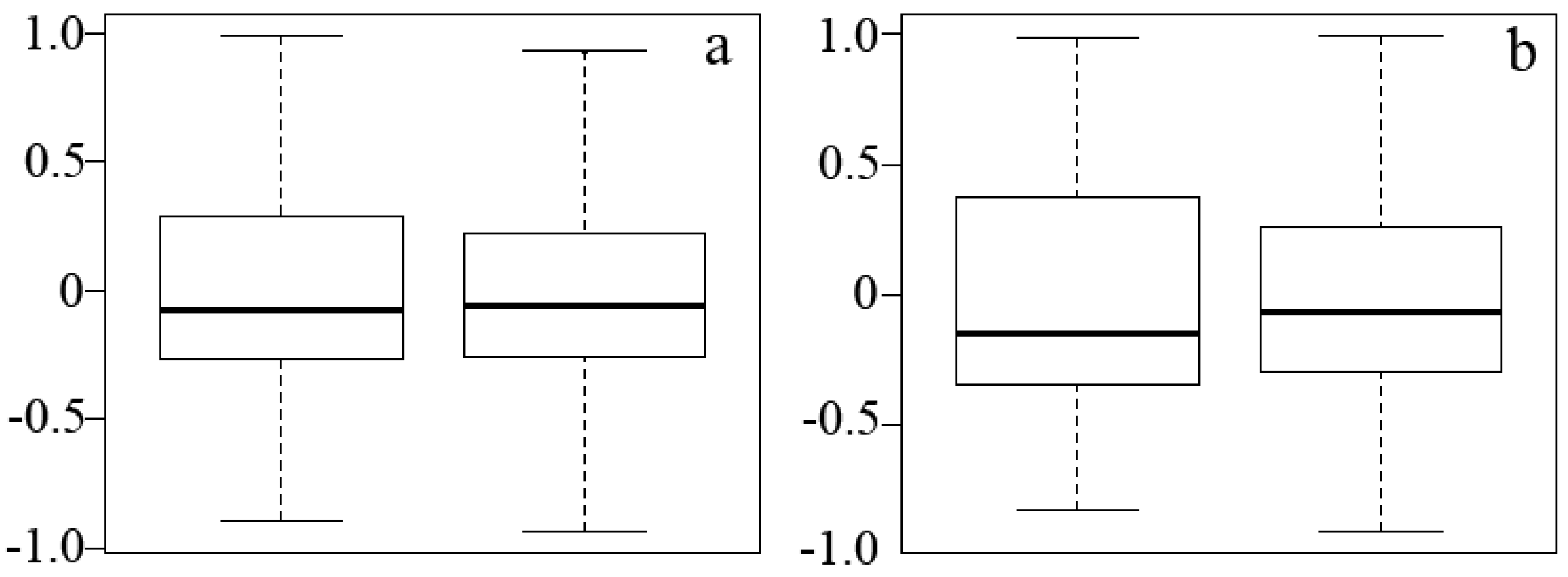
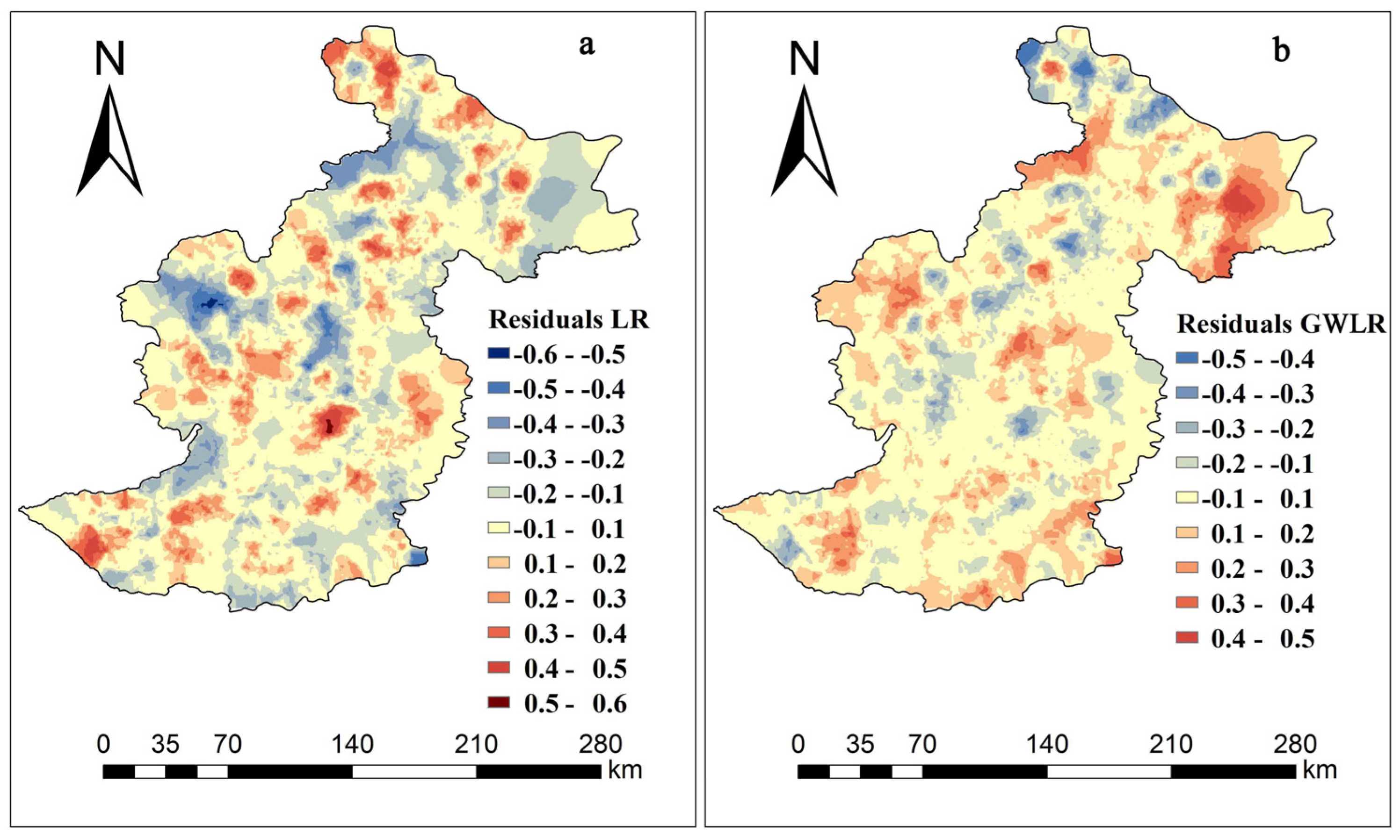
Both total residuals and spatial pattern of residuals for the LR and GWLR model were produced for the all variables test and significant variables test. The distribution of residual for both models appeared to be more or less symmetrical, with no serious bias; and the median residuals of the GWLR model were closer to 0 compared to the LR model (Figure 2). With regard to the spatial pattern of residuals, the GWLR model had the best fit; i.e., overall smaller residuals across the study area (Figure 3). In contrast, the overall residual of the LR final model was higher than that of GWLR and spatially uneven. The positive (under-prediction) and negative (over-prediction) residuals of the LR model were also clustered within the study area. The Moran’s I values were smaller for the GWLR than the LR model at different lag classes (Figure 4), indicating that the GWLR modelling had minimized residuals that might be caused by spatial autocorrelation.
3.2. Spatial Distribution of Fire-Drivers
Spatial interpolation of the estimated coefficient of explanatory variables included in the GWLR model was performed using the complete dataset to better understand their spatial pattern. The estimated coefficients of the GWLR model showed that distance to railway, distance to settlement, elevation, slope, population density and per capita GDP were negatively correlated with fire occurrence over the entire study area, while aspect and average monthly temperature correlated positively with fire occurrence in the majority of the study area. Other variables, including distance to road, forest type, distance to river, average relative humidity, and precipitation showed both positive and negative relationships over the study area (Figure 5).
The spatial heterogeneity of coefficients of selected significant variables, such as distance to railway, distance to residential area, average relative humidity, elevation and per capita GDP showed a negative correlation with forest fire occurrence across the study area (Figure 6). However, the influence area of other variables on fire occurrence concentrated in some specific parts of Yichun. The average monthly precipitation and distance to river only showed a significant positive relationship with forest fires in the south and north of Yichun, respectively. Both slope and distance to road have a strong negative correlation with fire occurrence at the center of the study area; distance to road also positively correlated to fire occurrence in the south and north of Yichun.
3.3. Fire Risk Classification
Maps of the likelihood of fire occurrence show that fire ignition was more likely to occur in the central region of Yichun, where the majority of forest-related human activities have taken place, with low possibility of fire detected around the peripheral regions (Figure 7A1,A2). In addition, fire risk zone maps derived from the cut-off values of LR and GWLR models showed more or less similar fire risk distribution in the study area; however, the GWLR model classified more high and moderate fire risk zones than the LR model (Figure 7B1,B2). The map obtained from both models shows that high fire risk zones were concentrated in the central region of Yichun; moderate risk zones surrounded the high risk zones, covering only minor regions of the study area; the low fire risk category covered the majority of the study area.
4. Discussion
The study demonstrates spatial variability in fire occurrence and its drivers in the UFEs, and the GWLR modelling approach captures this variability better than the LR. The GWLR model has better classification accuracy than non-spatial LR models (Table 2), with small spatial residuals(Figure 2, Figure 3 and Figure 4). This is attributed to the fact that the GWLR model is not designed to model spatial autocorrelation; but rather estimates local parameters explicitly at each data point, which can account for spatial heterogeneity [37]. Our result is consistent with previous studies that demonstrated higher classification accuracy with GWLR than a non-spatial logistic regression modelling approach [3,4]. The results also show that the causes of spatial variability in fire occurrence in UFEs are related to few anthropic and natural factors, notably infrastructure development, topography and weather variables. When studying factors that influence significantly the likelihood of fire occurrence, it is essential to consider regional variation in environmental and social conditions, as the same variables may function differently depending on the location and scale of analysis [49].
In the present study, the most important fire drivers in the UFEs were distance to railway, distance to river, slope, elevation and monthly average relative humidity. However, some variables such as distance to road, distance to settlement, precipitation, and per capita GDP are only identified as main fire drivers in the GWLR model. Fire occurrence was negatively correlated to distance to railway, distance to settlement, elevation, relative humidity and per capita GDP (Figure 5 and Figure 6). Railways reflect a transportation corridor in Yichun, and national fire records reveal that the majority of fire occurrences during this study period were accidental and negligent fires caused by human activities in and around railways, fire accidents by machinery, or lack of controlled burning activities near the tracks and railway infrastructure. Similar negative correlation between distance to railway and fire frequency was reported in the Upper Midwest states and Missouri and boreal forest in China [50,51,52]. On the contrary, Guo et al. [53] reported a positive relationship between fire and distance to railway in subtropical forest in China and Rodrigues et al. (2014) [3] reported both positive and negative relationships with spatial distribution in the study area. This discrepancy reflects that the effects of distance to railway on fire occurrences are site-specific. The negative relationship between distance to settlements and fire occurrence in the GWLR model suggests that ignition is most likely to occur near settlements, since most fires are caused by various human activities, such as slash burning and clearing agricultural residue. Our findings agree with previous studies that demonstrated significant negative correlations between fire occurrence and human settlement and activities [32,54,55,56,57].
Distance to road showed both significant positive (in the north and south of Yichun) and negative (in the central parts) influence on the likelihood of fire occurrence, revealing strong spatial variation in the influence of roads on fire occurrence. Distance to road has often been found to be related to human caused accidental or negligent fires [46,58,59]. Specifically, this risk appears to be higher in Wildland-Urban Interface (WUI) zones [15,60] where population and human infrastructure facilities are close to forested zones [61]. The positive relationship between road and fire occurrence in northern and southern Yichun is a surprising result and difficult to explain, as these areas are relatively far away from urban areas and road density is low. More fires occur in the forests in these areas and may correlate statistically with greater distance from roads.
Results from the present study show that some topographic and weather variables were found to be important drivers of fire in UFEs. It has been shown that lower elevation and flatter areas correlate positively with fire occurrence [62,63]. This is the case in many regions of China [30], as the majority of people reside at lower elevations in the Chinese boreal forest, and the same findings have been reported elsewhere [64,65,66]. Elevation likely influences fire frequency through surfacemoisture [67], species composition [68], and fuel moisture [69], which have been shown to increase with elevation. In addition, fire ignitions preferentially occur at lower elevations and at less steep slopes due to easy access by humans. Generally, steep slopes imply greater topographic roughness and are more difficult for humans to access [70]. As expected, average monthly relative humidity showed a significant negative correlation with fire occurrence over the whole of Yichun (Figure 6). High relative humidity induces an increase in moisture content of the fuel, thereby reducing the likelihood of fire. The GWLR model also identified a positive correlation between precipitation and fire occurrence, meaning high precipitation will increase the possibility of fire ignition. This might be related with increased growth of the herbaceous layer, which in turn increases the amount of fuel load. Similar findings were reported in other studies [71,72].
Socio-economic factors, population density and per capita GDP were negatively correlated with the likelihood of fire occurrence. Particularly, the probability of fire occurrence is lower in the northern part of the study area where per capita GDP is higher than the rural parts of the study area. One possible explanation would be a shift from traditional use of fire for heating and cooking to the use of modern fuels in a controlled environment. Similarly, as population density increases, availability of land resources decreases, which in turn reduces the likelihood of fire. Previous studies on the relationship between fire and GDP [36,73] have found similar results. As a whole, GDP is an important factor to consider at a regional scale, as the probability of fire occurrence is always greater when the per capita GDP is low. Among explanatory variables considered in the present study, vegetation type and aspect appeared to play no role in predicting the likelihood of fire occurrence in the study area. The relatively simple spatial composition of vegetation type in Yichun might be the cause of the weak relationship between vegetation type and fire occurrence, which is consistent with other studies [74,75]. Aspect is regarded as a critical factor of fire behavior, through its influence on wind speed, but was found to be poorly related to fire occurrence [76]. It is not surprising that aspect did not exhibit spatial variability as it is a pre-determined position in the landscape.
5. Conclusions and Management Perspectives
This study provides an improved understanding of the spatial variability of fire occurrence in Yichun, China, a typical UFE, as well as the relative importance of various underlying factors. Non-spatial global (LR) and spatial (GWLR) models were used to explore wildfire occurrence patterns and the main drivers. Compared to the LR model, the GWLR model demonstrated better performance, evidencing that spatially varying relationships improve the explanatory power of global LR models. The results show that both environmental and human factors influence the likelihood of fire occurrence in Yichun but the specific influence is spatially variable. The likelihood of fire occurrence was also mapped based on the two models, which in turn provided valuable information for improving fire prevention activities for local forest managers. This assessment contributes to the field of fire management and fire risk assessment in UFEs in China, as it quantitatively and spatially revealed the importance of accounting for local variation when modeling fire drivers.
Forest fire managers are often uncertain about the spatial locations where fire is likely to occur, thus linking fire ecology and management is paramount [77]. In this regard, the results of this study provide evidence about the importance of infrastructure and climate parameters as drivers of fire occurrence in the UFEs. From forest fire management perspectives, the findings have the following implications: (1) fire management policies should be developed based on spatial patterns of factors that will drive the maximum likelihood of fire occurrence; (2) allocation of resources for intensive fire prevention should be made based on the level of fire risk; (3) forest fire managers should implement fire prevention and fire suppression practices in high fire risk zones (such as railway tracks); and (4) planned burning would be a good option to reduce fuel loads and suppress unintended large fire, particularly around infrastructure facilities and settlements.
Acknowledgments
This research was funded by the Fujian Agriculture and Forestry University Funds for Distinguished Young Scholar (Grant No. xjq201613), Asia-Pacific Network for Sustainable Forest Management and Rehabilitation (APFnet Climate Research Project) Phase II, International Science and Technology Cooperation Program of Fujian Agriculture and Forestry University (KXB16008A). We also thank Brianne Riehl for further editing the manuscript.
Author Contributions
F.G., Z.S., and G.W. conceived and designed the experiments. X.Y., F.L., and H.L. collected and analyzed the data. F.G. and G.W. wrote the original draft. M.T. critically reviewed and edited the manuscript.
Conflicts of Interest
The authors declare no conflict of interest.
References
- Grogan, P.; Bruns, T.D.; Chapin, F.S. Fire effects on ecosystem nitrogen cycling in a Californian bishop pine forest. Oecologia 2000, 122, 537–544. [Google Scholar] [CrossRef] [PubMed]
- Liu, H.; Randerson, J.T.; Lindfors, J.; Chapin, F.S. Changes in the surface energy budget after fire in boreal ecosystems of interior Alaska: An annual perspective. J. Geophys. Res. 2005, 110, 1–12. [Google Scholar] [CrossRef]
- Rodrigues, M.; de-la-Riva, J.; Fotheringham, S. Modeling the spatial variation of the explanatory factors of human-caused wildfires in Spain using geographically weighted logistic regression. Appl. Geogr. 2014, 48, 52–63. [Google Scholar] [CrossRef]
- Martinez-Fernandez, J.; Chuvieco, E.; Koutsias, N. Modelling long-term fire occurrence factors in Spain by accounting for local variations with geographically weighted regression. Nat. Hazards Earth Syst. Sci. 2013, 13, 311–327. [Google Scholar] [CrossRef]
- Massada, A.B.; Radeloff, V.C.; Stewart, S.I.; Hawbaker, T.J. Wildfire risk in the wildland-urban interface: A simulation study in northwestern Wisconsin. For. Ecol. Manag. 2009, 258, 1990–1999. [Google Scholar] [CrossRef]
- Sanmiguelayanz, J.; Carlson, J.D.; Alexander, M.; Tolhurst, K.; Morgan, G.; Sneeuwjagt, R. Current Methods to Assess Fire Danger Potential. In Wildland Fire Danger Estimation and Mapping: The Role of Remote Sensing Data; World Scientific Publishing: Singapore, 2015; pp. 21–61. [Google Scholar]
- Costafreda-Aumedes, S.; Cardil, A.; Molina, D.M.; Daniel, S.N.; Mavsar, R.; Vega-Garcia, C. Analysis of factors influencing deployment of fire suppression resources in Spain using artificial neural networks. iForest 2015, 56, 609. [Google Scholar] [CrossRef]
- Renard, Q. Environmental susceptibility model for predicting forest fire occurrence in the Western Ghats of India. Int. J. Wildland Fire 2012, 21, 368–379. [Google Scholar] [CrossRef]
- Prestemon, J.P.; Chas-Amil, M.L.; Touza, J.M.; Goodrick, S.L. Forecasting intentional wildfires using temporal and spatiotemporal autocorrelations. Int. J. Wildland Fire 2012, 21, 743–754. [Google Scholar] [CrossRef]
- Lozano, F.J.; Suarez-Seoane, S.; Kelly, M.; Luis, E. A multi-scale approach for modeling fire occurrence probability using satellite data and classification trees: A case study in a mountainous Mediterranean region. Remote Sens. Environ. 2008, 112, 708–719. [Google Scholar] [CrossRef]
- Garcia, C.V.; Woodard, P.M.; Titus, S.J.; Adamowicz, W.L.; Lee, B.S. A logit model for predicting the daily occurrence of human caused forest fires. Int. J. Wildland Fire 1995, 5, 101–111. [Google Scholar] [CrossRef]
- Preisler, H.K.; Brillinger, D.R.; Burgan, R.E.; Benoit, J.W. Probability based models for estimation of wildfire risk. Int. J. Wildland Fire 2004, 13, 133–142. [Google Scholar] [CrossRef]
- Lozano, F.J.; Suarez-Seoane, S.; de-Luis, E. Assessment of several spectral indices derived from multi-temporal Landsat data for fire occurrence probability modeling. Remote Sens. Environ. 2007, 107, 533–544. [Google Scholar] [CrossRef]
- Hernandez-Leal, P.A.; Gonzalez-Calvo, A.; Arbelo, M.; Barreto, A.; Alonso Benito, A. Synergy of GIS and remote sensing data in forest fire danger modeling. IEEE J. Sel. Top. Appl. Earth Obs. Remote Sens. 2008, 1, 240–247. [Google Scholar] [CrossRef]
- Catry, F.X.; Rego, F.C.; Bacao, F.L.; Moreira, F. Modeling and mapping wildfire ignition risk in Portugal. Int. J. Wildland Fire 2009, 18, 921–931. [Google Scholar] [CrossRef]
- Chuvieco, E.; Aguado, I.; Yebra, M.; Nieto, H.; Salas, J.; Martin, M.P.; Vilar, L.; Martinez, J.; Martin, S.; Ibarra, P.; et al. Development of a framework for fire risk assessment using remote sensing and geographic information system technologies. Ecol. Model. 2010, 221, 46–58. [Google Scholar] [CrossRef]
- Reineking, B.; Weibel, P.; Conedera, M.; Bugmann, H. Environmental determinants of lightning vs. human-induced forest fire ignitions differ in a temperate mountain region of Switzerland. Int. J. Wildland Fire 2010, 19, 541–557. [Google Scholar] [CrossRef]
- Nieto, H.; Aguado, I.; Garcia, M.; Chuvieco, E. Lightning-caused fires in Central Spain: Development of a probability model of occurrence for two Spanish regions. Agric. For. Meteorol. 2012, 162–163, 35–43. [Google Scholar] [CrossRef]
- Zhang, H.J.; Han, X.Y.; Dai, S. Fire occurrence probability mapping of Northeast China with binary logistic regression model. IEEE J. Sel. Top. Appl. Earth Obs. Remote Sens. 2013, 6, 121–127. [Google Scholar] [CrossRef]
- Oliveira, S.; Oehler, F.; San-Miguel-Ayanz, J.; Camia, A.; Pereira, J.M.C. Modeling spatial patterns of fire occurrence in Mediterranean Europe using multiple regression and random forest. For. Ecol. Manag. 2012, 275, 117–129. [Google Scholar] [CrossRef]
- Rodrigues, M.; de-la-Riva, J. An insight into machine-learning algorithms to model human-caused wildfire occurrence. Environ. Model. Softw. 2014, 57, 192–201. [Google Scholar] [CrossRef]
- Guo, F.T.; Su, Z.W.; Wang, G.Y.; Sun, L.; Lin, F.F.; Liu, A.Q. Wildfire ignition in the forests of southeast china: Identifying drivers and spatial distribution to predict wildfire likelihood. Appl. Geogr. 2016, 66, 12–21. [Google Scholar] [CrossRef]
- Gitas, L.Z.; San-Miguel-Ayanz, J.; Chuvieco, E.; Camia, A. Advances in remote sensing and GIS applications in support of forest fire management. Int. J. Wildland Fire 2014, 23, 603–605. [Google Scholar] [CrossRef]
- Preisler, H.K.; Westerling, A.L.; Gebert, K.M.; Munoz-Arriola, F.; Holmes, T.P. Spatially explicit forecasts of large wildland fire probability and suppression costs for California. Int. J. Wildland Fire 2011, 20, 508–517. [Google Scholar] [CrossRef]
- Matthews, S.A.; Yang, T. Mapping the results of local statistics: Using geographically weighted regression. Demogr. Res. 2012, 26, 121–166. [Google Scholar] [CrossRef] [PubMed]
- Guo, F.T.; Selvaraj, S.; Lin, F.F.; Wang, G.Y.; Wang, W.H.; Su, Z.W.; Liu, A.Q. Geospatial information on geographical and human factors improved anthropogenic fire occurrence modeling in the Chinese boreal forest. Can. J. For. Res. 2016, 46, 582–594. [Google Scholar] [CrossRef]
- Oliveira, S.; Pereira, J.M.C.; San-Miguel-Ayanz, J.; Lourenco, L. Exploring the spatial patterns of fire density in Southern Europe using Geographically Weighted Regression. Appl. Geogr. 2014, 51, 143–157. [Google Scholar] [CrossRef]
- Zhang, H.J.; Qi, P.C.; Guo, G.M. Improvement of fire danger modelling with geographically weighted logistic model. Int. J. Wildland Fire 2014, 23, 1130–1146. [Google Scholar] [CrossRef]
- Shvidenko, A.Z.; Goldammer, J.G. Fire situation in Russia. IFFN 2001, 24, 41–59. [Google Scholar]
- Guo, F.T.; Innes, J.L.; Wang, G.Y.; Ma, X.Q.; Sun, L.; Hu, H.Q.; Su, Z.W. Historic distribution and driving factors of human-caused fires in the Chinese boreal forest between 1972 and 2005. J. Plant Ecol. 2015, 8, 1–10. [Google Scholar] [CrossRef]
- Hu, H.Q.; Li, N.; Sun, L.; San, L. Spatial and temporal distribution patterns of forest fires in Yichun, Heilongjiang Province. J. Northeast For. Univ. 2011, 39, 67–70. [Google Scholar]
- Chang, Y.; Zhu, Z.; Bu, R.; Chen, H.; Feng, Y.; Li, Y.; Hu, Y.; Wang, Z. Predicting fire occurrence patterns with logistic regression in Heilongjiang Province, China. Landsc. Ecol. 2013, 28, 1989–2004. [Google Scholar] [CrossRef]
- Kalabokidis, K.D.; Koutsias, N.; Konstantinidis, P.; Vasilakos, C. Multivariate analysis of landscape wildfire dynamics in a Mediterranean ecosystem of Greece. Area 2007, 39, 392–402. [Google Scholar] [CrossRef]
- Pew, K.L.; Larsen, C.P.S. GIS analysis of spatial and temporal patterns of human-caused wildfires in the temperate rain forest of Vancouver Island, Canada. For. Ecol. Manag. 2001, 140, 1–18. [Google Scholar] [CrossRef]
- Koutsias, N.; Martinez, J.; Chuvieco, E.; Alligower, B. Modeling wildland fire occurrence in southern Europe by a geographically weighted regression approach. In Proceedings of the 5th International Workshop on Remote Sensing and GIS Applications to Forest Fire Management: Fire Effects Assessment, Universidad de Zaragoza, Spain, 2005; pp. 57–60. [Google Scholar]
- Wang, Q.; Ni, J.; Tenhunen, J. Application of a geographically-weighted regression analysis to estimate net primary production of Chinese forest ecosystems. Glob. Ecol. Biogeogr. 2005, 14, 379–393. [Google Scholar] [CrossRef]
- Wu, W.; Zhang, L.J. Comparison of spatial and non-spatial logistic regression models for modeling the occurrence of cloud cover in northeastern Puerto Rico. Appl. Geogr. 2013, 37, 52–62. [Google Scholar] [CrossRef]
- Burnham, K.; Anderson, D.R. Model Selection and Multimodal Inference: A Practical Information-Theoretic Approach, 2nd ed.; Springer: New York, NY, USA, 2002. [Google Scholar]
- Hurvich, C.M.; Simono, J.F.; Tsai, C.L. Smoothing parameter selection in nonparametric regression using an improved Akaike information criterion. J. R. Stat. Soc. 1998, 60, 271–293. [Google Scholar] [CrossRef]
- Fielding, A.H.; Bell, J.F. A review of methods for the assessment of prediction errors in conservation presence/absence models. Environ. Conserv. 1997, 24, 38–49. [Google Scholar] [CrossRef]
- Zhou, X.H.; McClish, D.M.; Obuchowski, N.A. Statistical Methods in Diagnostic Medicine; John Wiley: Hoboken, NJ, USA, 2002. [Google Scholar]
- Franklin, J. Mapping Species Distributions; Cambridge University Press: New York, NY, USA, 2010. [Google Scholar]
- Hoyo, L.V.D.; Isabel, M.P.M.; Vega, F.J.M. Logistic regression models for human-caused wildfire risk estimation: Analysing the effect of the spatial accuracy in fire occurrence data. Eur. J. For. Res. 2011, 130, 983–996. [Google Scholar] [CrossRef]
- Legendre, P. Spatial autocorrelation: Trouble or new paradigm? Ecology 1993, 74, 1659–1673. [Google Scholar] [CrossRef]
- Kissling, W.; Carl, G. Spatial autocorrelation and the selection of simultaneous autoregressive models. Glob. Ecol. Biogeogr. 2008, 17, 59–71. [Google Scholar] [CrossRef]
- Zhang, H.; Qi, P.; Guo, G. Improvement of fire danger modelling with geographically weighted logistic model. Int. J. Wildland Fire 2014, 23, 1130–1146. [Google Scholar] [CrossRef]
- Wu, Z.; He, H.S.; Yang, J.; Liang, Y. Defining fire environment zones in the boreal forests of northeastern China. Sci. Total Environ. 2015, 518, 106–116. [Google Scholar] [CrossRef] [PubMed]
- Koutsias, N.; Martínezfernández, J.; Allgöwer, B. Do factors causing wildfires vary in space? Evidence from geographically weighted regression. GISci. Remote Sens. 2010, 47, 221–240. [Google Scholar] [CrossRef]
- Prasad, A.M.; Iverson, L.R.; Liaw, A. Newer classification and regression tree techniques: Bagging and random forests for ecological prediction. Ecosystems 2006, 9, 181–199. [Google Scholar] [CrossRef]
- Cardille, J.A.; Ventura, S.J.; Turner, M.G. Environmental and social factors influencing wildfires in the Upper Midwest, USA. Ecol. Appl. 2001, 11, 111–127. [Google Scholar] [CrossRef]
- Brosofske, K.D.; Cleland, D.T.; Saunders, S.C. Factors influencing modern wildfire occurrence in the Mark Twain National Forest, Missouri. South J. Appl. For. 2007, 31, 73–84. [Google Scholar]
- Guo, F.T.; Zhang, L.J.; Jin, S.; Tigabu, M.; Su, Z.W.; Wang, W.H. Modeling anthropogenic fire occurrence in the boreal forest of China using logistic regression and random forests. Forests 2016, 7, 1–14. [Google Scholar] [CrossRef]
- Guo, F.T.; Wang, G.Y.; Su, Z.W.; Liang, H.L.; Lin, F.F.; Liu, A.Q. What drives forest fire in Fujian, China? Evidence from logistic regression and random forests. Int. J. Wildland Fire 2016, 25, 505–519. [Google Scholar] [CrossRef]
- Martinez, J.; Vega-Garcia, C.; Chuvieco, E. Human-caused wildfire risk rating for prevention planning in Spain. J. Environ. Manag. 2009, 90, 1241–1252. [Google Scholar] [CrossRef] [PubMed]
- Dong, X.; Li, M.D.; Guo, F.S.; Lei, T.; Hui, W. Forest fire risk zone mapping from satellite images and GIS for Baihe Forestry Bureau, Jilin, China. J. For. Res. 2005, 16, 169–174. [Google Scholar] [CrossRef]
- Maingi, J.K.; Henry, M.C. Factors influencing wildfire occurrence and distribution in eastern Kentucky, USA. Int. J. Wildland Fire 2007, 16, 23–33. [Google Scholar] [CrossRef]
- Gowda, J.H.; Kitzberger, T.; Premoli, A.C. Landscape responses to a century of land use along the northern Patagonian forest-steppe transition. Plant Ecol. 2012, 213, 259–272. [Google Scholar] [CrossRef]
- Vasconcelos, M.J.P.; Sllva, S.; Tome, M.; Alvim, M.; Perelra, J.M.C. Spatial prediction of fire ignition probabilities: Comparing logistic regression and neural networks. Photogramm. Eng. Remot Sens. 2001, 67, 73–81. [Google Scholar]
- Yang, J.; He, H.S.; Shifley, S.R.; Gustafson, E.J. Spatial patterns of modern period human-caused fire occurrence in the Missouri Ozark Highlands. For. Sci. 2007, 53, 1–15. [Google Scholar]
- Syphard, A.D.; Radeloff, V.C.; Keeley, J.E.; Haqwbaker, T.J.; Clayton, M.K.; Stewart, S.I.; Hammer, R.B. Human influence on California fire regimes. Ecol. Appl. 2007, 17, 1388–1402. [Google Scholar] [CrossRef] [PubMed]
- Viegas, D.X.; Allgöwer, B.; Koutsias, N.; Eftichidis, G. Fire Spread and Urban Wildland Interface Problem. In Proceedings of the International Workshop on Forest Fires in the Wildland-Urban Interface and Rural Areas in Europe: An Intergral Planning and Management Challenge, Athens, Greece, 15–16 May 2003; Xanthopoulos, G., Ed.; MAICh: Chania, Greece, 2003; pp. 22–34. [Google Scholar]
- Gralewicz, N.J.; Nelson, T.A.; Wulder, M.A. Spatial and temporal patterns of wildfire ignitions in Canada from 1980 to 2006. Int. J. Wildland Fire 2012, 21, 230–242. [Google Scholar] [CrossRef]
- Kumar, S.; Meenakshi; Bairagi, G.D.; Vandana; Kumar, A. Identifying triggers for forest fire and assessing fire susceptibility of forests in Indian western Himalaya using geospatial techniques. Nat. Hazards 2015, 78, 203–217. [Google Scholar] [CrossRef]
- Flatley, W.T.; Lafon, C.W.; Grissino-Mayer, H.D. Climatic and topographic controls on patterns of fire in the southern and central Appalachian Mountains, USA. Landsc. Ecol. 2011, 26, 195–209. [Google Scholar] [CrossRef]
- Padilla, M.; Vega-Garcia, C. On the comparative importance of fire danger rating indices and their integration with spatial and temporal variables for predicting daily human-caused fire occurrences in Spain. Int. J. Wildland Fire 2011, 20, 46–58. [Google Scholar] [CrossRef]
- Gray, M.E.; Dickson, B.G.; Zachmann, L.J. Modelling and mapping dynamic variability in large fire probability in the lower Sonoran Desert of south-western Arizona. Int. J. Wildland Fire 2014, 23, 1108–1118. [Google Scholar] [CrossRef]
- Hayes, G.L. Influences of Altitude and Aspect on Daily Variations in Factors of Forest Fire Danger; U.S. Department of Agriculture: Washington, DC, USA, 1941; p. 39.
- Haugo, R.D.; Hall, S.A.; Gray, E.M.; Gonzalez, P.; Bakker, J.D. Influences of climate, fire, grazing, and logging on woody species composition along an elevation gradient in the eastern Cascades, Washington. For. Ecol. Manag. 2010, 260, 2204–2213. [Google Scholar] [CrossRef]
- Holden, Z.A.; Jolly, W.M. Modeling topographic influences on fuel moisture and fire danger in complex terrain to improve wildland fire management decision support. Forest. Ecol. Manag. 2011, 262, 2133–2141. [Google Scholar] [CrossRef]
- Guyette, R.P.; Muzika, R.M.; Dey, D.C. Dynamics of an anthropogenic fire regime. Ecosystems 2002, 5, 472–486. [Google Scholar]
- Knies, C.; Elm, M.T.; Klar, P.J.; Stehr, J.; Hofmann, D.M.; Romanov, N. Fire–rainfall relationships in Argentine Chaco savannas. J. Arid. Environ. 2010, 74, 1319–1323. [Google Scholar]
- Pausas, J.G. Changes in fire and climate in the eastern Iberian Peninsula (Mediterranean Basin). Clim. Chang. 2004, 63, 337–350. [Google Scholar] [CrossRef]
- Aldersley, A.; Murray, S.J.; Cornell, S.E. Global and regional analysis of climate and human drivers of wildfire. Sci. Total Environ. 2011, 409, 3472–3481. [Google Scholar] [CrossRef] [PubMed]
- Johnson, E.A.; Larsen, C.P.S. Climatically induced change in fire frequency in the southern Canadian Rockies. Ecology 1991, 72, 194–201. [Google Scholar] [CrossRef]
- Wu, Z.; He, H.S.; Yang, J.; Liu, Z.; Liang, Y. Relative effects of climatic and local factors on fire occurrence in boreal forest landscapes of northeastern China. Sci. Total. Environ. 2014, 493, 472–480. [Google Scholar] [CrossRef] [PubMed]
- Sebastián-López, A.; Salvador-Civil, R.; Gonzalo-Jiménez, J. Integration of socio-economic and environmental variables for modelling long-term fire danger in Southern Europe. Eur. J. For. Res. 2008, 127, 149–163. [Google Scholar] [CrossRef]
- Burrows, N.D. Linking fire ecology and fire management in south-west Australian forest landscapes. For. Ecol. Manag. 2008, 255, 2394–2406. [Google Scholar] [CrossRef]
Figure 1.
Maps of the study area, fire locations and fire cause distribution. “Human induced” cause in the pie chart represents both intentional and unintentional fires due to various human activities.
Figure 1.
Maps of the study area, fire locations and fire cause distribution. “Human induced” cause in the pie chart represents both intentional and unintentional fires due to various human activities.

Figure 2.
Residual box plots of the LR and GWLR models in the all variable test (a) and significant variable test (b). The left box in both panels represents the LR model, and the right box represents the GWLR model.
Figure 2.
Residual box plots of the LR and GWLR models in the all variable test (a) and significant variable test (b). The left box in both panels represents the LR model, and the right box represents the GWLR model.

Figure 3.
Spatial distribution of model residuals of LR (a) and GWLR (b) models.

Figure 4.
Correlograms for residuals of LR and GWLR models in the all variable test (a) and significant variable test (b).
Figure 4.
Correlograms for residuals of LR and GWLR models in the all variable test (a) and significant variable test (b).
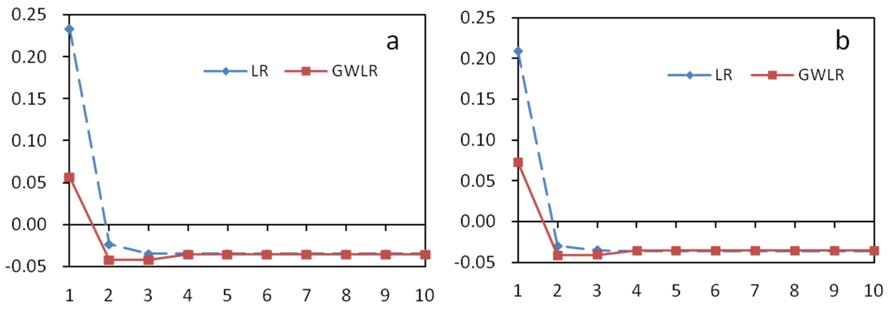
Figure 5.
Spatial patterns of regression coefficients for explanatory variables in the GWLR model. The abbreviated variable names are the same as in Table 1. The estimated coefficient was displayed with a warm color (orange to red) when positive and with a cold color (blue) when the coefficient was negative.

Figure 6.
Spatial patterns of estimated GWLR coefficient for selected significant variables. If the t-value of the estimated coefficient for a particular variable is <−1.96 or >1.96, then the variable had a significant effect on fire occurrence; otherwise the variable was considered as insignificant. Negative coefficients are mapped with cold colors (blue), and positive coefficients are mapped with warm colors (orange to red). The abbreviated variable names are the same as in Table 1.

Figure 7.
Maps of the likelihood of fire occurrence (A1,A2) and fire risk classes (B1,B2) from LR and GWLR models. The cut-off values for fire risk zone classification are 0.39 and 0.35 for the LR and GWLR models, respectively.
Figure 7.
Maps of the likelihood of fire occurrence (A1,A2) and fire risk classes (B1,B2) from LR and GWLR models. The cut-off values for fire risk zone classification are 0.39 and 0.35 for the LR and GWLR models, respectively.


Table 1.
Variables included as predictors in the model.
| Variable Name | Code | Data Type/Resolution | Data Description and Extraction | Source |
|---|---|---|---|---|
| Climate Average monthly precipitation | Preci_m_avg | Raster/1 km | The climate factors of each fire point and control point were retrieved from the HADCM2 climate model. The HADCM2 climate model, developed by the Hadley Centre for Climate Research and Prediction, was used in coupled mode. The original dataset was collected from the Intergovernmental Panel on Climate Change (IPCC) and rescaled. The corresponding monthly climate factors for each fire and control point were retrieved from ArcGIS19.0 environment. | Earth System Science Data Sharing Platform, China |
| Average monthly relative humidity | RH_m_avg | |||
| Average monthly temperature | Temp_m_avg | |||
| Topographic Elevation | Elev | Raster/25 m | Elevation, slope and aspect values were retrieved from the Digital Elevation Model (DEM) data with resolution of 25 m. Elevation and slope values for each fire and control point were used directly in the modelling process. The aspect was categorised as flat, North (315–45°), East (45–135°), South (135–225°) and West (225–315°). The proportion of each variant in the study area was calculated and the corresponding value for each fire and control point was used to develop the model. | National Administration of Surveying, Mapping and Geoinformation of China, 2002 |
| Slope | Slope | |||
| Aspect | Aspect | |||
| Vegetation Forest type | Forest type | Raster/1 km | Forest vegetation types for each fire and non-fire point were extracted from the vegetation map (1 km resolution). Accordingly, four categories were identified: (1) needle leaf deciduous and needle leaf evergreen trees; (2) broadleaf deciduous trees and broadleaf deciduous shrubs; (3) grass and agricultural crops; and (4) urban construction land, permanent wetland and barren or sparsely vegetated land. These vegetation types were extracted from the vegetation map layer for each fire point and control point in ArcGIS 10.0; and the proportion of each vegetation type located in a fire or control point was used during modelling. | The Cold and Arid Regions Science Data Center, China, 2000 |
| Infrastructure Distance to river | Dis_ river | Vector/1:250,000 | Basic geographic information was obtained from the National Administration of Surveying, Mapping and Geoinformation of China. The data were collected in 2000. The variables were retrieved based on a 1:250,000 Digital Line Graphic (DLG) map and included: distance to nearest railway, distance to nearest road and distance to nearest river. | National Administration of Surveying, Mapping and Geoinformation of China, 2002 |
| Distance to railway | Dis_ railway | |||
| Distance to road | Dis_road | |||
| Distance to settlement | Dis_sett | |||
| Socio-economic Per Capita GDP | CGDP | Raster/1 km | Two variables represent the Per Capita GDP and annual population density of the study area. This data was then correlated with fire points and control points using the ArcGIS Raster Extraction tool. | The Road of Revitalization-Thirty Years of Reform, Heilongjiang, 2009 Statistical Yearbook of China 2000, 2001 |
| Density of population | Den_Pop |
The codes chosen may not include the whole description of the variable for simplicity purposes.
Table 2.
Coefficient estimates of all variables and significant variables tests for the logistic regression (LR) and geographically weighted logistic regression (GWLR) models.
Table 2.
Coefficient estimates of all variables and significant variables tests for the logistic regression (LR) and geographically weighted logistic regression (GWLR) models.
| Statistics | βintercept | βDis_railway | βDis_road | βDis_sett | βDis_river | βVeg_type | βSlop | βAspect | βElev | βRH | βTemp | βPreci | βCGDP | βDen_pop |
|---|---|---|---|---|---|---|---|---|---|---|---|---|---|---|
| All variables | ||||||||||||||
| LR model | ||||||||||||||
| Estimate | 9.931 | −0.013 | 0.147 | −0.211 | 0.026 | 0.098 | −0.029 | 4.268 | −0.004 | −0.019 | 0.036 | 0.011 | −0.0002 | −0.219 |
| S.D. | 1.101 | 0.005 | 0.031 | 0.027 | 0.012 | 0.279 | 0.017 | 3.204 | 0.0006 | 0.012 | 0.015 | 0.075 | 0.00003 | 0.030 |
| Estimate − 1s.d. | 8.830 | −0.018 | 0.116 | −0.238 | 0.014 | −0.181 | −0.046 | 1.064 | −0.0046 | −0.031 | 0.021 | −0.064 | −0.00023 | −0.249 |
| Estimate + 1s.d. | 11.032 | −0.008 | 0.178 | −0.184 | 0.038 | 0.377 | −0.012 | 7.472 | −0.0034 | −0.007 | 0.051 | 0.086 | −0.00017 | −0.189 |
| GWLR model | ||||||||||||||
| Minimum | 7.335 | −0.064 | −0.147 | −0.240 | −0.006 | −0.446 | −0.033 | 0.041 | −0.00583 | −0.064 | −0.0003 | −0.188 | −0.0003 | −0.233 |
| 25% quartile | 8.518 | −0.056 | 0.056 | −0.202 | −0.0003 | −0.277 | −0.024 | 1.514 | −0.0043 | −0.035 | 0.031 | −0.132 | −0.0003 | −0.211 |
| Mean | 9.817 | −0.038 | 0.078 | −0.184 | 0.013 | −0.120 | −0.019 | 2.451 | −0.00358 | −0.019 | 0.045 | −0.065 | −0.0002 | −0.202 |
| Median | 9.745 | −0.039 | 0.089 | −0.179 | 0.005 | −0.132 | −0.020 | 2.403 | −0.0034 | −0.014 | 0.050 | −0.062 | −0.0002 | −0.201 |
| 75% quartile | 11.268 | −0.020 | 0.136 | −0.164 | 0.029 | 0.059 | −0.016 | 3.484 | −0.00278 | −0.002 | 0.064 | −0.001 | −0.00008 | −0.192 |
| Maximum | 12.449 | −0.014 | 0.173 | −0.145 | 0.044 | 0.143 | −0.002 | 4.580 | −0.00212 | 0.004 | 0.071 | 0.063 | −0.00002 | −0.176 |
| Significant variables | ||||||||||||||
| LR model | ||||||||||||||
| Estimate | 0.047 | −0.015 | - | - | −0.033 | - | −0.063 | - | −0.004 | 0.018 | - | 0.099 | - | - |
| p−value | 0.969 | <0.001 | - | - | <0.0001 | - | <0.001 | - | <0.001 | 0.005 | - | 0.03 | - | - |
| S.D. | 0.308 | 0.004 | - | - | 0.007 | - | 0.011 | - | 0.0002 | 0.006 | - | 0.034 | - | - |
| GWLR model | ||||||||||||||
| Minimum | 4.740 | −0.068 | −0.159 | −0.241 | −0.003 | - | −0.036 | - | −0.006 | −0.058 | - | 0.037 | −0.0004 | - |
| 25% quartile | 5.333 | −0.061 | 0.055 | −0.206 | 0.002 | - | −0.028 | - | −0.004 | −0.048 | - | 0.045 | −0.0004 | - |
| Mean | 5.824 | −0.043 | 0.080 | −0.190 | 0.015 | - | −0.023 | - | −0.004 | −0.041 | - | 0.069 | −0.0003 | - |
| Median | 5.965 | −0.044 | 0.089 | −0.187 | 0.006 | - | −0.024 | - | −0.003 | −0.039 | - | 0.061 | −0.0004 | - |
| 75% quartile | 6.341 | −0.024 | 0.142 | −0.171 | 0.030 | - | −0.018 | - | −0.003 | −0.035 | - | 0.086 | −0.0002 | - |
| Maximum | 6.707 | −0.018 | 0.178 | −0.150 | 0.049 | - | −0.005 | - | −0.002 | −0.030 | - | 0.116 | −0.0001 | - |
The abbreviated variable names are the same as in Table 1.
Table 3.
Comparison of goodness of fit and prediction accuracy of LR and GWLR models in all variables (A.V.) and significant variables (S.V.) tests.
Table 3.
Comparison of goodness of fit and prediction accuracy of LR and GWLR models in all variables (A.V.) and significant variables (S.V.) tests.
| Dataset | Model | AIC | AICc | SSE | AUC | Cut-Off | Prediction Accuracy (%) | ||||||||
|---|---|---|---|---|---|---|---|---|---|---|---|---|---|---|---|
| Training Set (60% Data) | Validation (40% Data) | ||||||||||||||
| A.V. | S.V. | A.V. | S.V. | A.V. | S.V. | A.V. | S.V. | A.V. | S.V. | A.V. | S.V. | A.V. | S.V. | ||
| Sample 1 | LR | 1603.59 | 1665.92 | 1603.85 | 1666.05 | 257.14 | 339.09 | 0.827 | 0.683 | 0.438 | 0.381 | 77.8 | 68.1 | 76.3 | 68.1 |
| GWLR | 1504.49 | 1542.29 | 1507.32 | 1543.80 | 227.32 | 238.54 | 0.865 | 0.853 | 0.433 | 0.415 | 79.7 | 77.4 | 85.2 | 83.8 | |
| Sample 2 | LR | 1615.02 | 1637.89 | 1615.28 | 1638.03 | 258.97 | 336.73 | 0.814 | 0.669 | 0.400 | 0.384 | 78.0 | 67.9 | 75.1 | 63.9 |
| GWLR | 1516.63 | 1486.21 | 1519.49 | 1496.31 | 229.27 | 210.74 | 0.854 | 0.879 | 0.336 | 0.385 | 77.2 | 80.1 | 83.9 | 86.6 | |
| Sample 3 | LR | 1599.73 | 1626.39 | 1599.99 | 1626.50 | 256.66 | 332.46 | 0.823 | 0.693 | 0.395 | 0.414 | 77.3 | 69.2 | 75.3 | 69.8 |
| GWLR | 1491.39 | 1471.72 | 1496.36 | 1480.67 | 220.07 | 210.39 | 0.870 | 0.883 | 0.395 | 0.364 | 79.8 | 80.4 | 85.8 | 86.1 | |
| Sample 4 | LR | 1567.02 | 1615.77 | 1567.28 | 1615.91 | 251.37 | 339.67 | 0.833 | 0.686 | 0.444 | 0.395 | 78.3 | 68.0 | 75.7 | 67.7 |
| GWLR | 1451.52 | 1516.59 | 1469.29 | 1518.07 | 224.21 | 234.06 | 0.866 | 0.855 | 0.419 | 0.431 | 80.0 | 77.9 | 85.9 | 83.6 | |
| Sample 5 | LR | 1560.97 | 1819.49 | 1561.23 | 1819.56 | 248.80 | 355.93 | 0.833 | 0.596 | 0.424 | 0.338 | 77.9 | 65.3 | 75.2 | 48.2 |
| GWLR | 1478.60 | 1664.90 | 1480.13 | 1665.16 | 226.20 | 267.36 | 0.863 | 0.814 | 0.383 | 0.422 | 78.0 | 75.1 | 84.9 | 83.8 | |
| Complete dataset | LR | 2670.82 | 3331.48 | 2670.97 | 3331.53 | 431.58 | 568.22 | 0.820 | 0.676 | 0.429 | 0.410 | 77.5 | 67.8 | - | - |
| GWLR | 2534.87 | 2616.65 | 2535.87 | 2617.27 | 398.32 | 415.33 | 0.847 | 0.835 | 0.440 | 0.355 | 78.5 | 73.7 | - | - | |
AIC = Akaike’s information criterion; AICc = AIC with a correction for finite sample sizes; SSE = sum of squared errors of prediction; AUC = area under the curve. For the complete dataset, the data were not divided into training or validation datasets, so we only calculated one prediction accuracy for the all variables and significant variables tests.
© 2017 by the authors. Licensee MDPI, Basel, Switzerland. This article is an open access article distributed under the terms and conditions of the Creative Commons Attribution (CC BY) license (http://creativecommons.org/licenses/by/4.0/).
Share and Cite
MDPI and ACS Style
Guo, F.; Su, Z.; Tigabu, M.; Yang, X.; Lin, F.; Liang, H.; Wang, G. Spatial Modelling of Fire Drivers in Urban-Forest Ecosystems in China. Forests 2017, 8, 180. https://doi.org/10.3390/f8060180
AMA Style
Guo F, Su Z, Tigabu M, Yang X, Lin F, Liang H, Wang G. Spatial Modelling of Fire Drivers in Urban-Forest Ecosystems in China. Forests. 2017; 8(6):180. https://doi.org/10.3390/f8060180
Chicago/Turabian StyleGuo, Futao, Zhangwen Su, Mulualem Tigabu, Xiajie Yang, Fangfang Lin, Huiling Liang, and Guangyu Wang. 2017. "Spatial Modelling of Fire Drivers in Urban-Forest Ecosystems in China" Forests 8, no. 6: 180. https://doi.org/10.3390/f8060180
Note that from the first issue of 2016, this journal uses article numbers instead of page numbers. See further details here.