Application of UAV Photogrammetric System for Monitoring Ancient Tree Communities in Beijing


1
Precision Forestry Key Laboratory of Beijing, Beijing Forestry University, Beijing 100083, China
2
Daxing District Gardening and Greening Bureau, Beijing 102600, China
3
Beijing Daxing Fruit and Forestry Institute, Beijing 102600, China
*
Author to whom correspondence should be addressed.
Forests 2018, 9(12), 735; https://doi.org/10.3390/f9120735
Submission received: 18 October 2018
/
Revised: 22 November 2018
/
Accepted: 23 November 2018
/
Published: 24 November 2018
(This article belongs to the Special Issue Forestry Applications of Unmanned Aerial Vehicles (UAVs) 2019)
Abstract
:Ancient tree community surveys have great scientific value to the study of biological resources, plant distribution, environmental change, genetic characteristics of species, and historical and cultural heritage. The largest ancient pear tree communities in China, which are rare, are located in the Daxing District of Beijing. However, the environmental conditions are tough, and the distribution is relatively dispersed. Therefore, a low-cost, high-efficiency, and high-precision measuring system is urgently needed to complete the survey of ancient tree communities. By unmanned aerial vehicle (UAV) photogrammetric program research, ancient tree information extraction method research, and ancient tree diameter at breast height (DBH) and age prediction model research, the proposed method can realize the measurement of tree height, crown width, and prediction of DBH and tree age with low cost, high efficiency, and high precision. Through experiments and analysis, the root mean square error (RMSE) of the tree height measurement was 0.1814 m, the RMSE of the crown width measurement was 0.3292 m, the RMSE of the DBH prediction was 3.0039 cm, and the RMSE of the tree age prediction was 4.3753 years, which could meet the needs of ancient tree survey of the Daxing District Gardening and Greening Bureau. Therefore, a UAV photogrammetric measurement system proved to be capable when applied in the survey of ancient tree communities and even in partial forest inventories.
1. Introduction
Ancient trees are the cornerstone of the natural, agricultural, and urban ecosystems on earth [1,2,3,4,5]. The investigation of ancient tree communities is of great scientific value to the study of biological resources, plant distribution, environmental change, genetic characteristics of species, and historical and cultural heritage [6,7]. In view of the specific situation of the ancient tree community survey, few unique survey patterns have been formed. At present, the traditional forest survey pattern is mainly used in the survey of ancient tree communities. The Daxing District of Beijing has the world’s rarest ancient pear tree communities. For the purpose of protecting and managing ancient trees, preventing the malicious and illegal felling of ancient trees, and strengthening the information management of ancient trees, the Daxing District Gardening and Greening Bureau hopes to carry out ancient tree communities monitoring every year. As more than 100,000 pear trees and 40,000 ancient pear trees are scattered over more than 400 km2, great difficulties have arisen in the investigation of ancient tree communities. In addition, the Daxing District Gardening and Greening Bureau can only conduct the survey of ancient pear trees within one month before the Pear Flower Festival every year. Therefore, the high efficiency and real-time performance of the survey of ancient tree communities becomes particularly critical.
Traditional forest survey patterns include ground surveys and aerial remote sensing surveys [8,9]. As ground survey equipment, an electronic total station can accurately measure the three-dimensional coordinates, height, diameter at breast height (DBH), stem volume, and canopy volume of an individual tree [10]. Forest intelligent surveying and mapping instruments, which are portable and internal-external integrated, can be applied in the measurement of height, DBH, and volume of an individual tree. In addition, stand average height, stand average DBH, stand density, and stand volume can be estimated by the angle gauge measure function embedded in the program [11]. A forest telescope intelligent dendrometer is capable of measuring height and DBH of an individual tree from a long range. In addition, stand parameters can be estimated by using the embedded micro sample plot measure function [12]. Even though the above survey instruments have the function of stand parameter estimation, they are more suitable for the accurate measurement of an individual tree than a large-scale forest survey. A terrestrial laser scanning (TLS) system, as an efficient and high-precision measurement method, has gradually become an important means of conducting a forest survey and can visually measure stand structure parameters in three dimensions [13,14]. The main purpose of TLS is to improve the efficiency of forest sample plot monitoring. With the help of the point cloud, automatic acquisition replaces manual measurement of tree attributes, which mainly include tree height, DBH, crown width, and coordinates [15]. The line of sight of TLS is not limited to only a few meters. Several scanning locations are required rather to avoid gaps in the point cloud due to occlusion from terrain or vegetation [16]. This limitation means that using TLS point cloud data to describe large areas of forest space is time-consuming and costly [17].
Airborne laser scanning (ALS) is a good solution for large areas of forest investigation. The ALS systems can generate 3D point cloud data to describe tree height and canopy structure and use other methods to build the relationship between tree heights, canopy structures, and other forest attributes [18]. Many research results showed that the accuracy and precision of the forest survey were satisfying in obtaining forest attributes, such as forest volume and forest biomass, using ALS systems [19,20,21,22,23]. More and more people choose to use high-resolution digital aerial images to generate 3D data just like ALS and apply it to the forest survey [24,25,26]. The cost of unmanned aerial vehicle (UAV) photogrammetric measurement systems is more acceptable compared to ALS, and attributes such as species composition, maturity, and health status can be acquired through images. Many studies have shown that UAV photogrammetric measurement systems can generate 3D data and the combination of the digital surface model (DSM) and digital elevation model (DEM) can deduce the height of a canopy on the ground, thus producing a canopy height model (CHM) [27]. Generally, UAV photogrammetric measurement systems rely on a ground control point (GCP), which is regarded as a source of reliable georeferencing information [28]. Furthermore, in the UAV photogrammetric measurement systems, additional GCPs are often used to calibrate the location parameters [28]. In general, UAV photogrammetric measurement systems require more than 30 control points per square kilometer, which is undoubtedly extremely difficult and inefficient in a complex forest environment [29]. Therefore, we need a kind of UAV photogrammetric measurement system that can meet the forestry survey requirements. In addition, without a proper sensor geometric calibration, the GCPs will not provide enough accuracy for coordinate correction and that will affect the final 3D model accuracy. Nan An and others imported the converted TIFF images into the Agisoft Photoscan program to generate an orthophoto by correcting perspective distortion [30]. Dongwook Kim and others used Pix4Dmapper software to auto-compensate the principal point and radial distortion by processing the bundle block adjustment [31].
Forest modeling is a type of ecological modeling. With the development of forestry informatization, the relationship between forest modeling and high spatial resolution three-dimensional (3D) remote sensing has become closer [32,33,34,35]. Temuulen T. Sankey and others have proposed combining light detection and ranging (LiDAR) data and hyperspectral data for ecological modeling and subtle environmental change detection [36,37]. Remote sensing techniques, in combination with forest modeling, which can be applied to estimate forest biomass and carbon stock [38,39] and to monitor forest harvest and recruitment [40], are widely used in ecosystem process modeling [41]. Remote sensing techniques such as LiDAR can be combined with the algorithm for individual tree detection [42,43,44] to obtain tree height and canopy area. Many studies have shown that the use of linear mixed models can well establish the correlation between tree height, canopy area, and DBH [45]. In addition, in the forest modeling study, if DBH and tree height are known, tree growth modeling combined with forest environment can predict tree age well [46,47]. However, the development of these two models requires an expensive monitoring system to effectively monitor the forest environment [48]. The survey of ancient tree communities in Daxing District requires high efficiency and low cost. Therefore, a new forest modeling method is needed to predict DBH and tree age.
This study aims to solve the following main problems:
- On the premise of ensuring the accuracy of forestry survey, it is necessary to study a continuous photogrammetric algorithm and software suitable for monitoring ancient tree communities.
- Using existing technology and algorithms, it is necessary to study the effective and accurate extraction of forest information from the point cloud data.
- Because of the specific situation of ancient tree communities, it is necessary to study the ancient tree structure relationship model and ancient tree growth model to estimate the DBH and age.
2. Materials and Methods
2.1. Profile of Study Sites
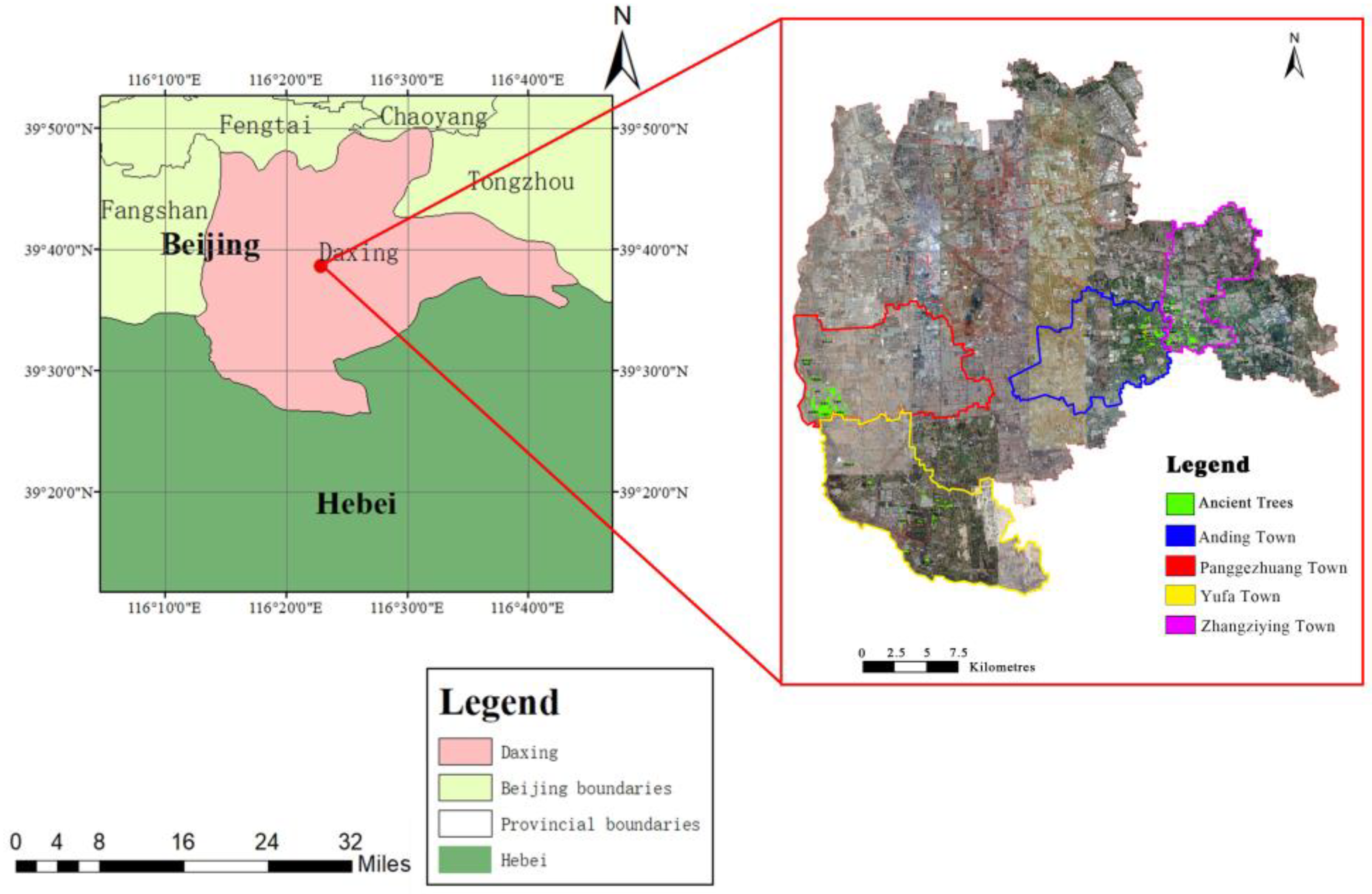
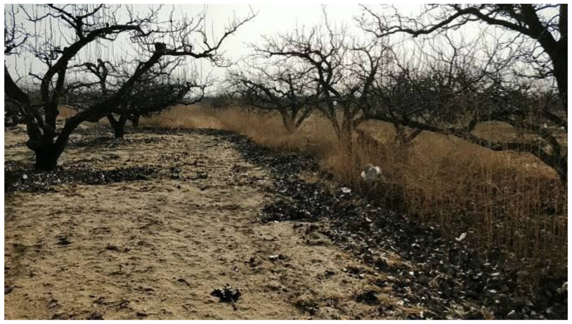
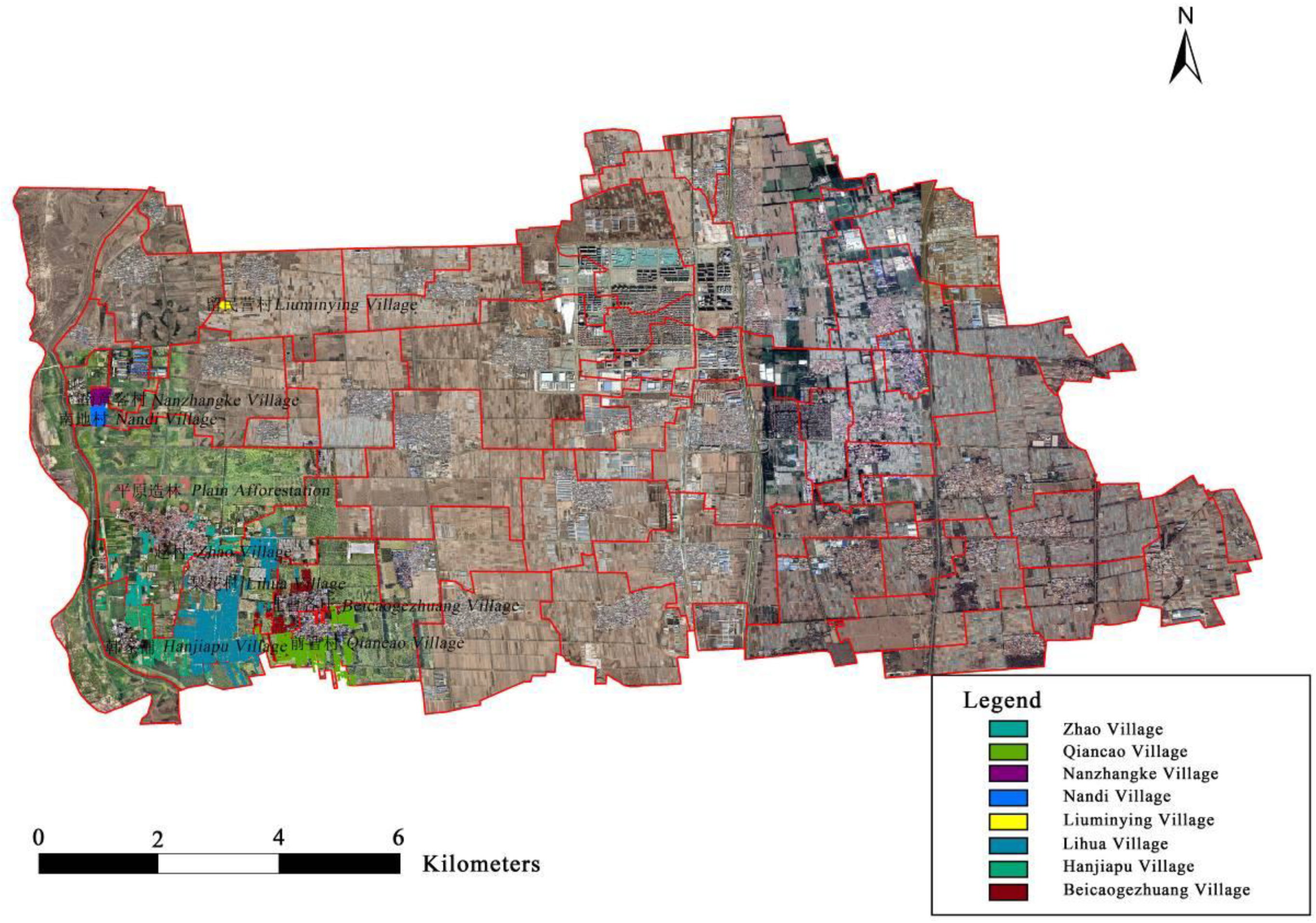
Daxing District (Figure 1) is located in the south area of Beijing, with Tongzhou District to the east, Gu’an County and Bazhou City in the Hebei province in the south, the Yongding River in the west, and the Fangshan, Fengtai, and Chaoyang districts in the north. It has an east longitude of 116°13′–116°43′ and a north latitude of 39°26′–39°51′. The whole district is on the Yongding River alluvial plain. The terrain gradually slopes from the west to the southeast, with an altitude between 14 and 52 m. There are six main rivers in the Daxing District, including the Yongding, Liangshui, Tiantang, Dalong, Xiaolong, and Xinfeng. The Beijing Daxing Wanmu pear orchard is the largest ancient pear tree community with the largest planting area, the earliest flowering, and the most varieties around Beijing. The central area is located in Lihua Village, where more than 40,000 ancient pear trees (Figure 2) have been preserved for over 50 years. There are more than 40 varieties of pear trees in this area, one of which is 417 years old and has been named “gold yellow” by an emperor of Qing dynasty. From Appendix A, we can see the distribution of ancient trees in each town in Daxing District.
2.2. Technical Information
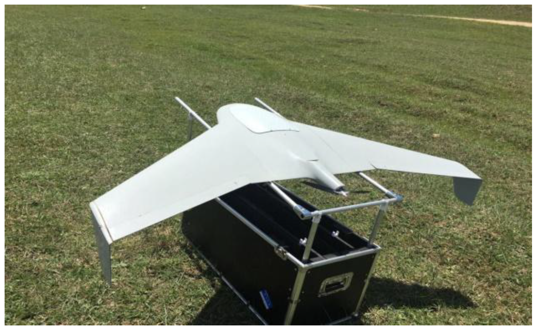
In this study, by using the YS-500 Fixed-Wing UAV (Figure 3 and Table 1, Beijing Global Forest Technology Co. LTD, Beijing, China) and Sony-A7R camera (Table 2), aerial images of Panggezhuang Town were obtained. The flight area was about 49 km2, and the ground resolution was better than 5 cm. A total of 4984 images were taken through taking off and landing six times, with an average height of 331 m. The fore-and-aft overlap of route planning was 65%, and the side overlap was 75%.
Control points were measured by Yinhe I RTK (Real Time Kinematic) measurement system (made in China South Surveying & Mapping Instrument Company). The specific parameters of RTK are shown in Table 3.
2.3. Research on the Improved UAV Photogrammetric Program
SfM is the abbreviation of structure from motion, which is a valuable tool for generating 3D models from 2D images. It is developed from computer vision and conventional photogrammetry. Unlike conventional photogrammetry, SfM uses algorithms to identify matching features in the set of overlapping images and to calculate the camera position and direction in accordance with the difference of the multiple matching features [49,50]. Based on these calculations, the overlapping images can be used to reconstruct the “sparse” or “rough” three-dimensional point cloud model of the captured object. The model obtained by the SfM method can be further refined by a multi-view stereo (MVS) algorithm, so as to complete the workflow of SfM-MVS [51].
The SfM-MVS method is relatively inexpensive, both in terms of hardware and software requirements. It is faster than other digital measurements in the field and is a process almost independent of spatial scales. In addition, the SfM-MVS can also produce 3D point cloud data with high precision, high density, and high resolution. In some cases, it may even catch up with the terrestrial laser scanner [49].
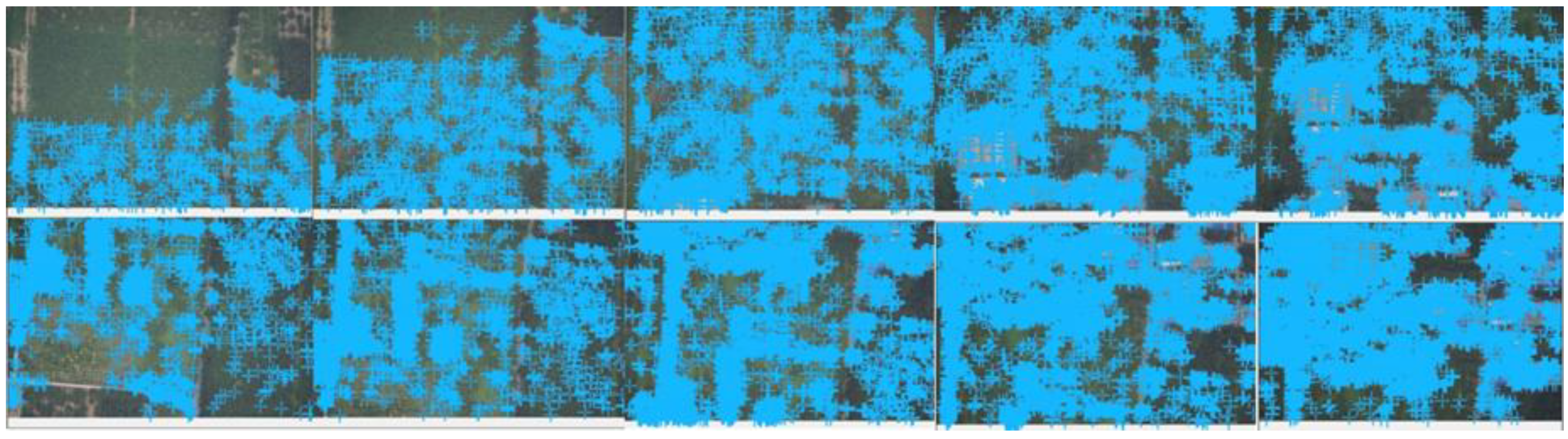
In this study, the SfM-MVS method was used to detect the feature points of the image, and the scale-invariant feature transform (SIFT) algorithm (Figure 4) was used to detect feature points and generate feature vectors. By identifying the correspondence between feature points on different images, we screen out the image pairs with overlapping parts. Then, the matching was carried out according to the feature vectors, and the RANSAC (random sample consensus) algorithm was used to delete the connection of the conflicting geometric features of corresponding feature points.
The regional network bundle adjustment method of aerial triangulation contains a beam of light composed of an image as the basic unit of adjustment and the collinearity formula of central projection as the basic formula of adjustment [52,53]. Through the rotation and translation of every light beam in space, the best intersection of the light from the common points between the models can be achieved, and the entire region can be optimally incorporated into the known control point coordinate system [54,55]. The advantage of this algorithm is that it only takes more than four GCPs for the free network bundle adjustment method and the system bundle adjustment method, so as to obtain the correction number of the images, improve the efficiency of the field work, and minimize the measurement error.
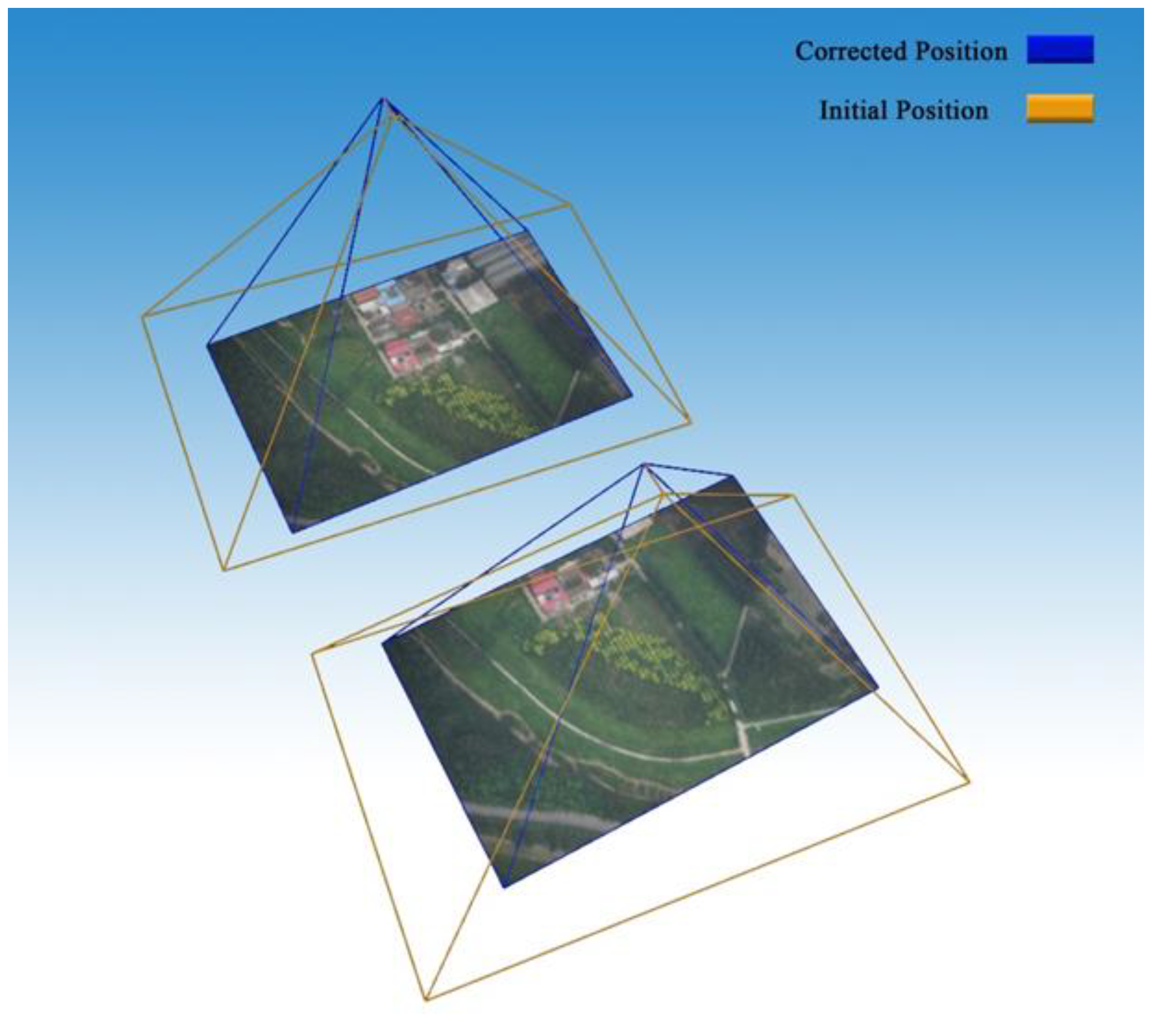
is longitudinal tilt, is lateral tilt, and is swing angle. are longitude, latitude, and altitude. Given the profile of the test area, UAV POS (Positioning and Orientation System) data (, , , , , ) and ground control point ) (n ≥ 4), free network adjustment was first conducted (Figure 5). Nine control points were arranged in the four corners of the rectangle, the center of the four edges and the center of the rectangle. Among them, () and () are the corresponding image point to image i + 1 and image i, respectively. and are the corresponding scale factor to image i + 1 and image i, respectively. and are the elements of exterior orientation of the POS data in the image. i + 1, and are the elements of exterior orientation of POS data in image i. is the initial value of the rotation matrix composed of the elements of exterior orientation of POS data in image i. is the initial value of the rotation matrix composed of the elements of exterior orientation of POS data in image i + 1. Formula (1) can be obtained by substituting the values of three corresponding image points.
j stands for corresponding image point. and , and , , and are calculated beforehand. , and f are coordinates of the corresponding image point. Therefore, we can get the corrections, such as , , , , , and .
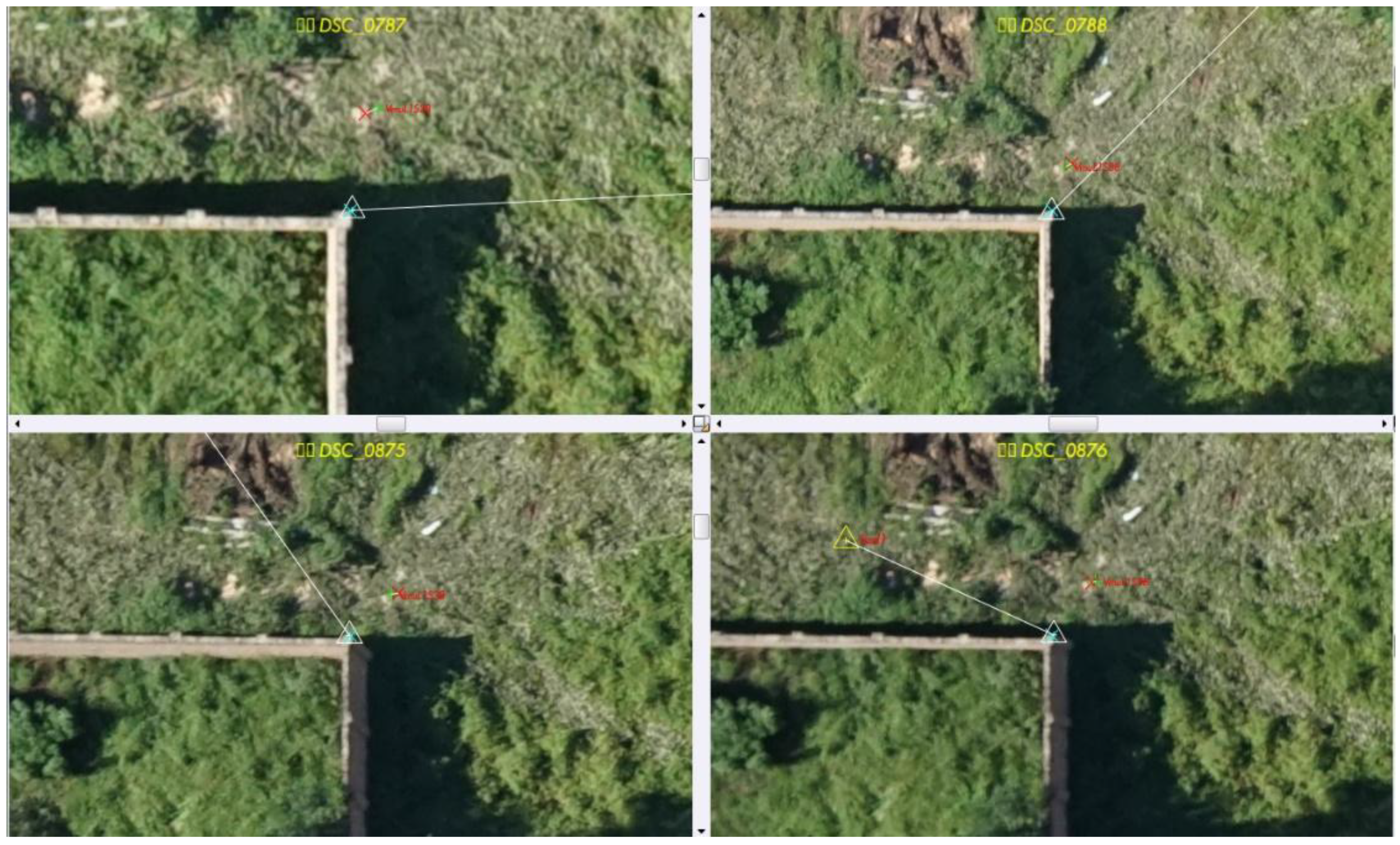
The selection and positioning of the image control points (Figure 6) is to accurately indicate the position of the image control point on the image. It is the basis of image interpretation and measurement. In the selection and positioning of image control points, the intersection of linear ground objects and the corner of ground objects are generally selected.
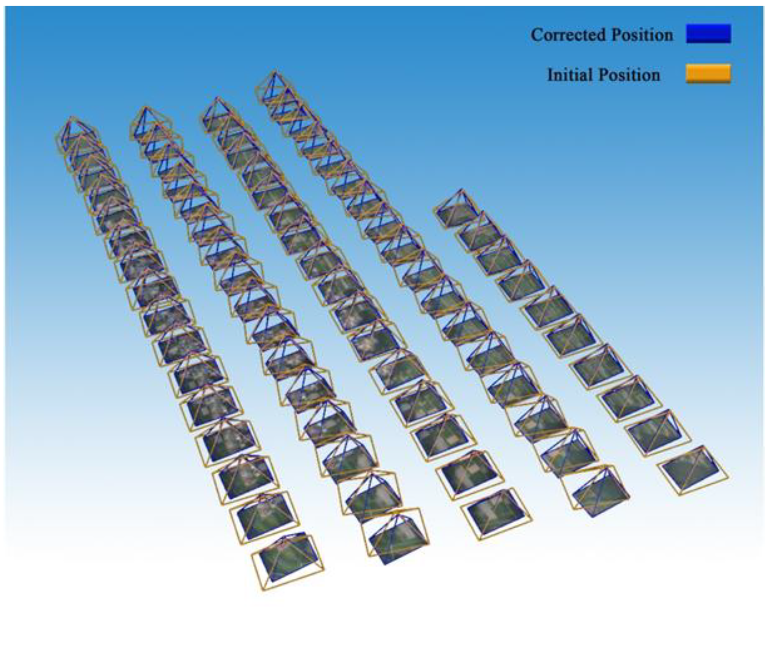
According to the correction between images (Figure 7), the adjustment value of each image center is calculated, and the coordinates of each ground control point in the independent coordinate system of images are then calculated. We convert the image coordinate system to the ground coordinate system, so as to obtain the final correction value after the system bundle adjustment method.
From the above, based on the development platform of Microsoft Visual Studio 2010, using C# language, we independently developed software called “New UAV Bundle Adjustment” for image matching and POS correction. The image and POS data processed by this software were imported into Pix4Dmapper software for three-dimensional (3D) points cloud modeling. Pix4Dmapper comes from the Swiss company Pix4D, which is the research result of the world-class research institute EPFL (Swiss Federal Institute of Technology in Lausanne).
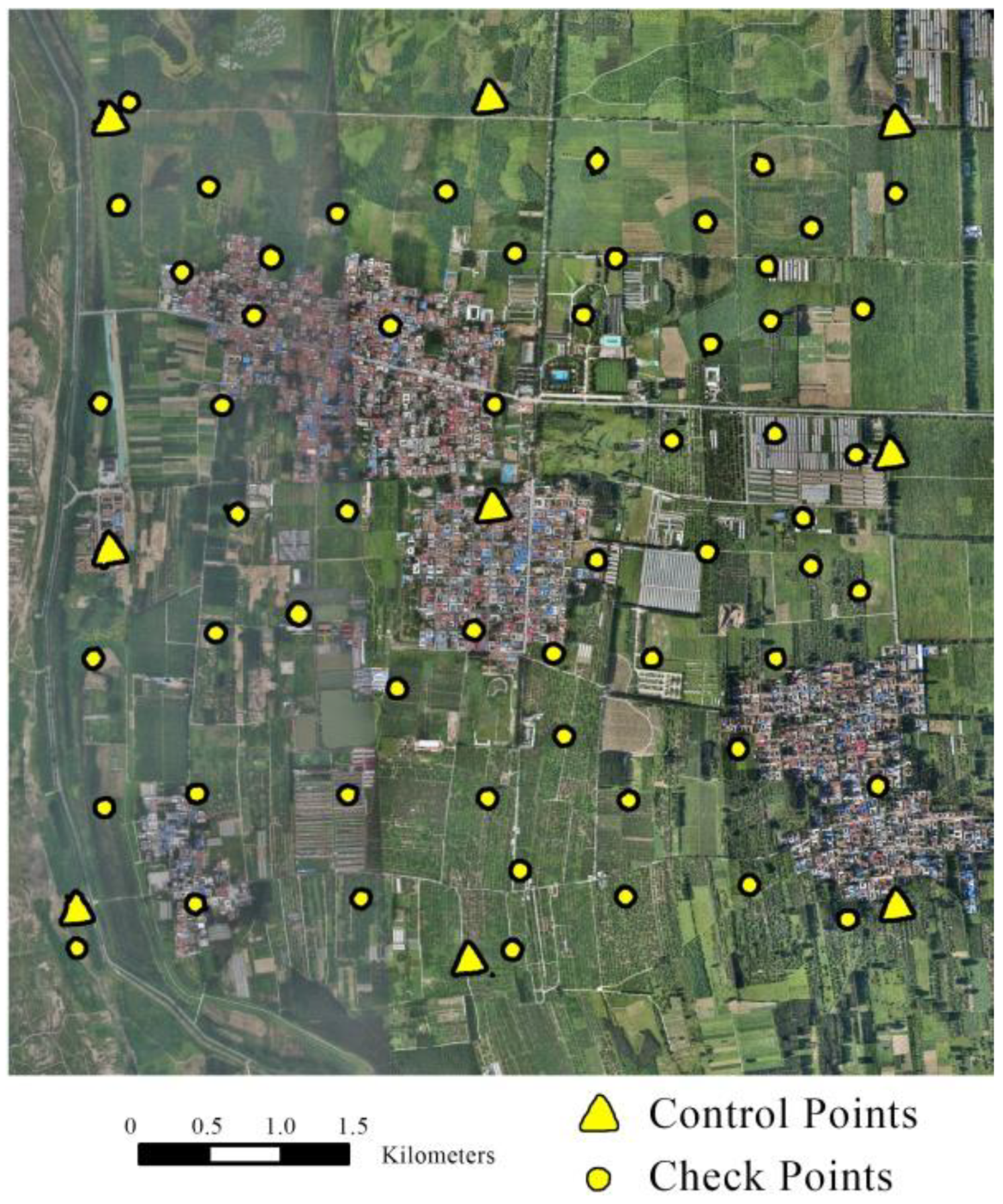
The number of control points and the layout position will have a great influence on the precision of aerial triangulation. To verify the accuracy of improved UAV photogrammetric program in this study, nine control points were set up in Panggezhuang Town (Figure A1), and a total of 68 field control points were collected by RTK. The flight area was about 49 km2. The same height points were set up on the four sides and the center line of the region. Considering that this test area was a more regular rectangular region, nine points were arranged in the four corners of the rectangle, the center of the four edges, and the center of the rectangle. The remaining 59 points were precision check points. Data acquisition was based on the same camera (Table 2). Data Source A used the improved bundle adjustment for calculation, and Data Source B adopted the conventional aerial measurement method. The layout scheme is shown in Figure 8.
The precision of orientation points and check points by using the bundle adjustment was evaluated via field measurement. The difference value between the calculated value of ground coordinate and the measured coordinate was considered to be the true error. The root mean square error was calculated according to Formula (2).
In the formula, and were the root mean square error (RMSE) of points in the X and Y directions. was the root mean square error of the points in the elevation. was the root mean square error of the points in the plane. , , and were the measured coordinate values of the check points. , , and were the calculated coordinate values of check points by using the bundle adjustment.
2.4. Research on the Ancient Tree Information Extraction Method
The image matching point cloud based on the UAV platform can cover large areas and generate high-density accurate point cloud, and the cost is relatively low. An image matching point cloud is a series of inhomogeneous and discrete point sets in space, which contains certain texture information. A DSM can be obtained through the processing of point cloud data, and a DEM can be obtained through the filtering process [49]. As the image point cloud is a passive remote sensing product, it does not have multiple echoes, and it is difficult to obtain accurate DEM data directly in densely vegetated areas. Therefore, it is necessary to conduct research and analysis in information extraction of forest. This study used LiDAR 360 (Beijing Digital Green Earth Technology Co. LTD, Beijing, China) software to extract ancient tree information.
2.4.1. Classification of Ground Point Based on Point Cloud Data
(1) Point cloud denoising. In the process of point cloud acquisition, some noise points will appear due to equipment inaccuracy and environmental factors. Removal of noise points before data processing can improve data accuracy and reduce the error caused by noise points [56]. The noise removal algorithm adopted in this study includes the high threshold method, the isolated point search method, and the low point search method.
(2) Ground point classification. Ground point refers to the point below ground vegetation or the ground building. The basic idea of extracting the ground point is to assume that the lowest point in an area is its ground point and search these local lowest points to form the initial surface. On this basis, the relationship between other points and the initial surface can be valued. If it conforms to a certain relationship, it will be regarded as the ground point for classification, which is dealt with by multiple iterations. Different geomorphic features have different iterative algorithms and given thresholds [49]. In this study, a hierarchical robust linear predictive filtering algorithm, a morphological filtering algorithm based on gradient, and a TIN stepwise encryption algorithm were used.
2.4.2. Generation of Raster Data from Point Clouds
(1) DSM generation. Point cloud data are irregular three-dimensional discrete points, which need to be interpolated to generate a three-dimensional model with continuous changes [49]. The algorithms used in this study include inverse distance weighted (IDW) interpolation, Kriging interpolation, natural neighbor interpolation, and radial basis function interpolation.
(2) DEM generation. Discrete ground points are interpolated to generate DEM [49]. Firstly, the ground point cloud is rasterized, the ground point is then extracted by the local minimum search window algorithm, and the raster data is interpolated using the TIN interpolation algorithm.
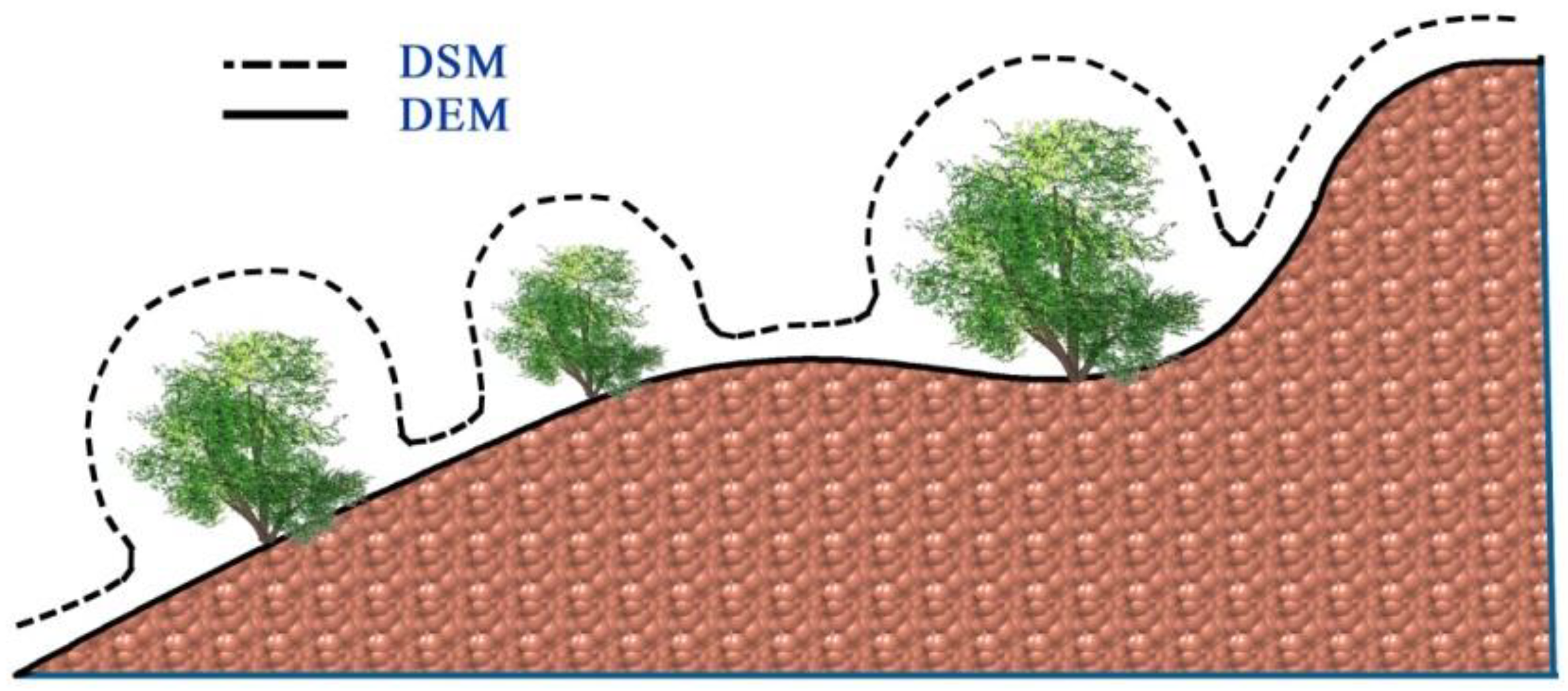
(3) CHM generation. The canopy height model (CHM) is a high-resolution raster dataset that maps the height of the tree to a continuous surface, where each pixel represents the height of the tree above the ground. The method of obtaining CHM is the subtraction of DSM and DEM [49]. Ground fluctuation in the study of ancient tree community causes the bottom of the trees to not be on the same horizontal surface, and the introduction of CHM can solve this problem well. CHM reduces the calculation of tree height to a plane, which can conveniently reflect the information of tree height, as shown in Figure 9.
2.4.3. Segmentation of Individual Ancient Tree
The three-dimensional point cloud is rasterized and transformed into CHM based on the 3D point cloud, from which information such as tree height and crown width can be obtained. In the individual tree segmentation of pear trees, the model algorithm of seed region growth is adopted [49]. The basic method is to form convex hull polygons based on CHM and then reconstruct the canopy along the two-dimensional convex hull with the normalized image point cloud, so as to achieve the purpose of individual tree segmentation. The detailed process is as follows.
(1) A sliding window to detect the location of seed point was defined. The minimum threshold of tree height will be set during processing. When the value is greater than the minimum threshold detected in slide detection, this point is considered as the seed point. (2) The points on CHM are marked and divided into seed points and non-seed points. (3) Four adjacent points near a seed point are searched for to determine whether the seed point to each point is greater than the set crown width threshold on the plane and whether the height is greater than the height threshold. If the above two points are satisfied, it will be regarded as a new seed point, which will be reclassified and processed several times until all seed points and non-seed points are classified. (4) Marked seed points were used as the center to establish a two-dimensional convex envelope marking boundary. (5) The final boundary contour of the generated point boundary polygon is used as the basis to segment the normalized point cloud data and achieve the purpose of individual tree segmentation.
According to image data and impression of the field situation, the position of missed, excessive, and false detection points were edited. The false seed points could be deleted. The excessive seed points could be deleted and the corrected seed points could be reserved. The missed seed points could be added. Then, the individual tree could be segmented. The central location of the tree could be obtained by the center coordinate of prominent position.
2.5. Research on the Ancient Tree DBH and Age Prediction Model
The height–crown-width–DBH model and “3 speed 2 inflection points” optimum condition growth model of pear trees were developed based on the measured data from a pear tree survey in Lihua Village, Daxing District. In combination with a UAV photogrammetric tree measurement system, the DBH and age of individual trees can be estimated accurately.
2.5.1. Building of the Height–Crown-Width–DBH Model
Data of fixed plots are usually affected by the within-plot and temporal correlation. In order to solve this potential problem of autocorrelation, linear mixed models were fitted to the data by including a random effect of plot (to model spatial correlation) in the model and by specifying an autoregressive error structure (to model temporal correlation) [45]. The fixed plot data of this study is the previous survey data of pear tree communities in Lihua Village (Appendix A, Figure A1), with a total of 1484 pear trees, including only DBH, tree height, and crown width. In 2014, Local Forestry Station investigators made use of the Diameter Ruler and Electronic Total Station (NTS 362R, China South Surveying & Mapping Instrument Company, Guangdong, China) to measure the DBH, height, and crown breadth of pear trees. Therefore, it is more suitable to use the nonlinear model. Referring to the common height–DBH model and crown width–DBH model, the height–crown-width–DBH model (Formula (3)) is obtained.
is the diameter at breast height, is the tree height, and is the crown width. and are the factors to establish the correlation between tree height and DBH. and are the factors to establish the correlation between crown width and DBH.
2.5.2. Building of the “3 Speed 2 Inflection Points” Optimum Condition Growth Model
The growth data in this study were 39 ancient pear trees in Lihua Village obtained by specimens of trees, including the annual diameter growth of different types of pear trees. Commonly used tree growth modeling includes the logistic model, the Mitscherlich model [57], the Gompertz model, the Korf model [58], and the Richards model [59]. In the above model fitting process, the sample data will be regarded as a mean tree of the same site and environment. Therefore, it is necessary to propose a growth model, which can not only fit the sample data at different sites and under different environments but also fit the overall growth trend of the sample data. Tree growth consists of three basic processes, namely cell division, cell elongation, and cell differentiation. Theoretically, the growth potential of cells and tissues is unlimited, and their growth should always be exponential. However, since the internal interactions between individual cells or organs limit growth [60], the growth process of trees is divided into the juvenile period, the medium period, and the near-mature period. In this study, the three stages were summarized as “3 speed 2 inflection points,” and the overall growth trend was relatively stable. Different tree growth indexes were assigned to each sample data, which is the composite index of site index, structure index, and growth rate index. By selecting the optimal tree growth index and the tree growth model, the optimal tree growth can be obtained, as shown in Formula (4).
is the DBH, is the age of the tree, , , , , , and are the parameters of the tree growth model of the overall sample data. is the tree growth index model of each independent sample data, and , , and are the factors of this model.
3. Results
3.1. Experiment Preparation
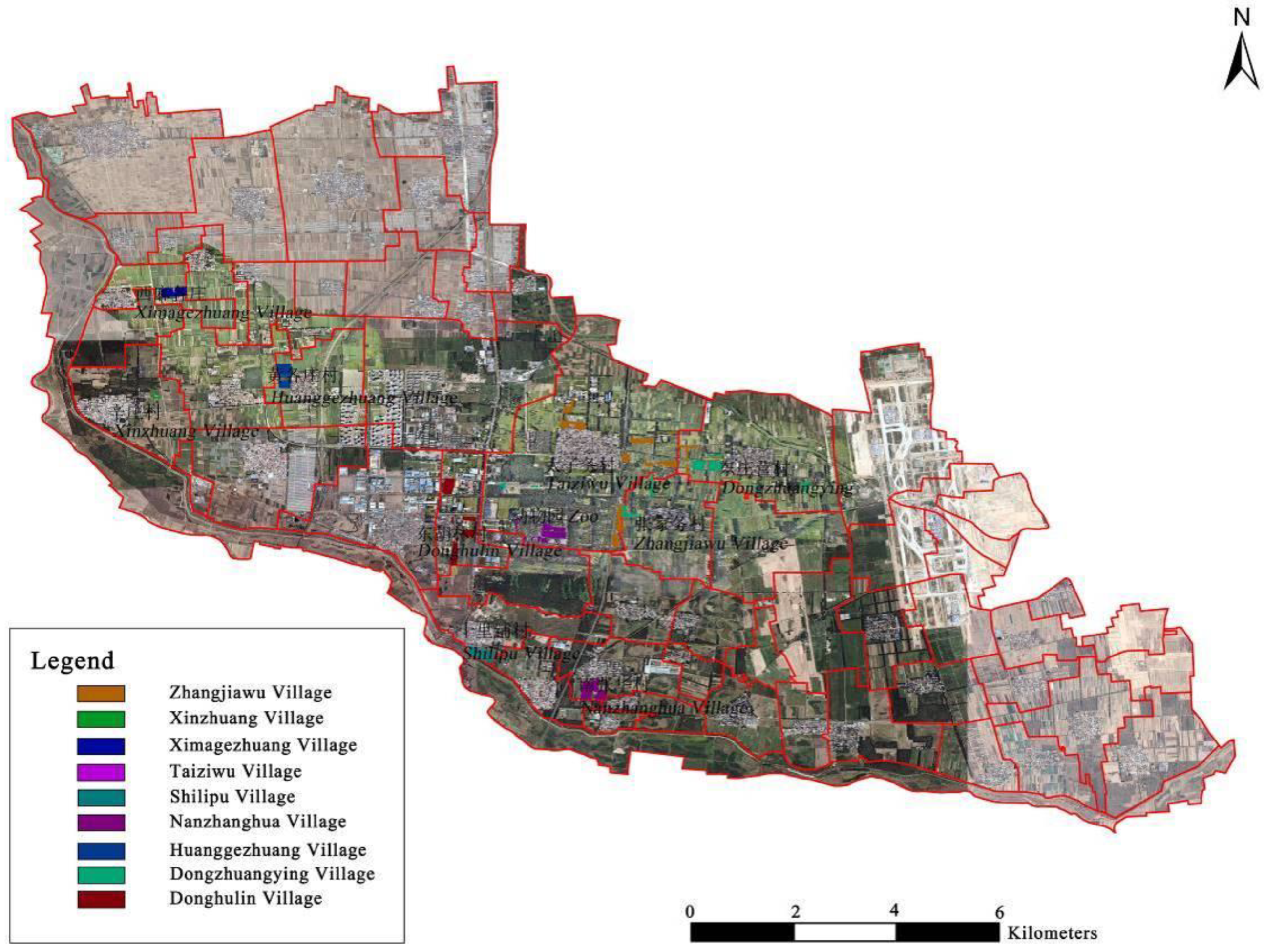
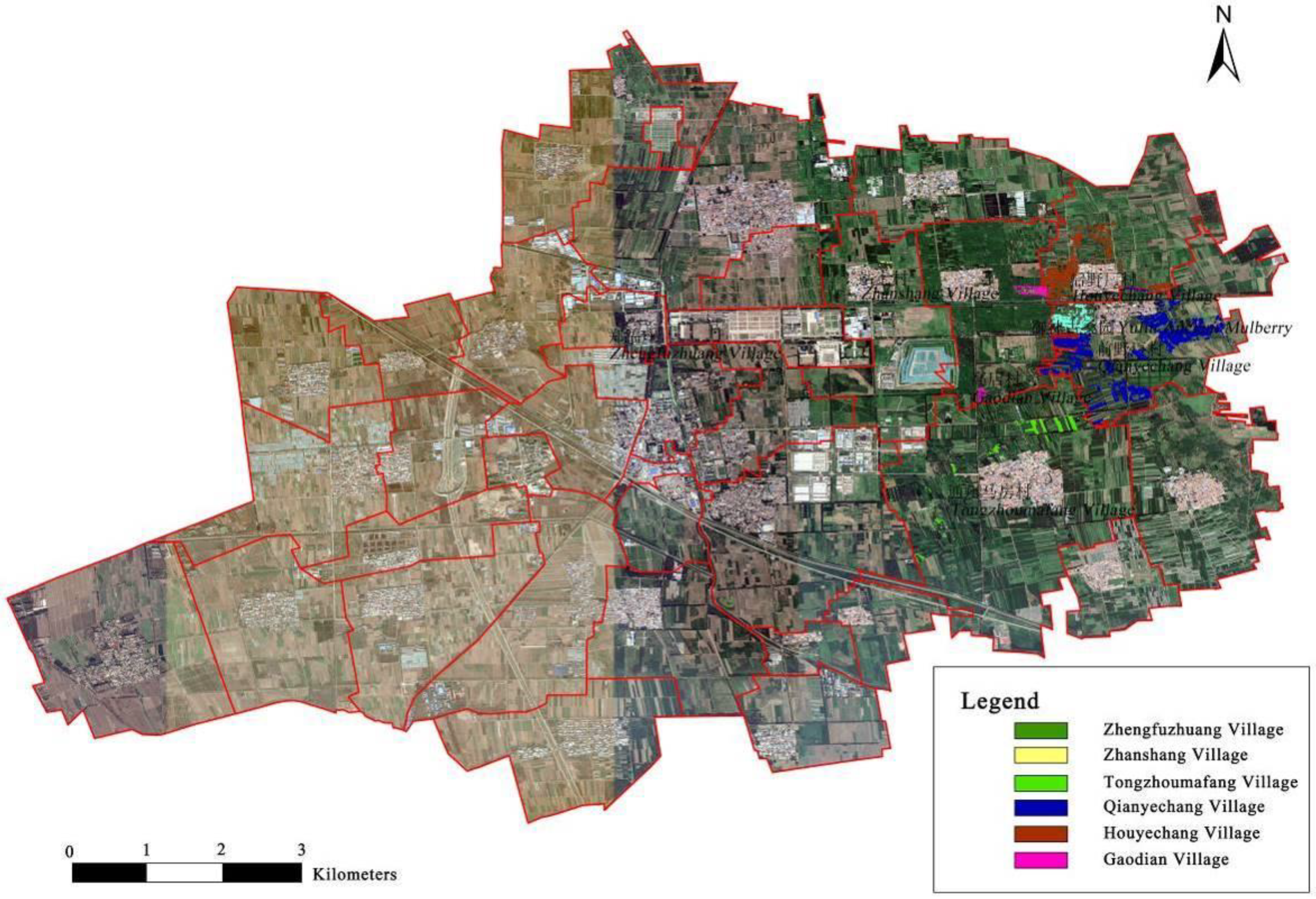
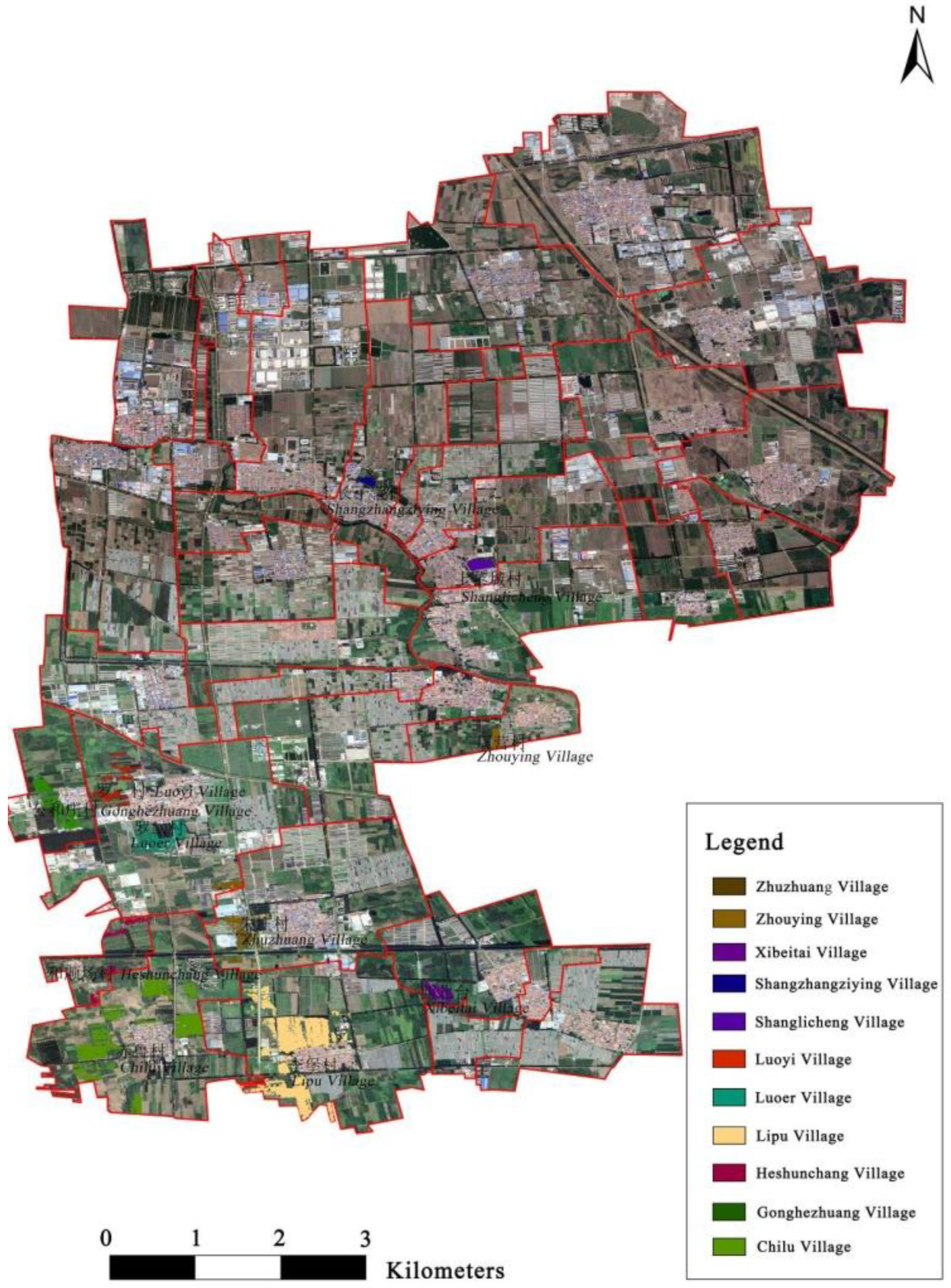
We choose Beicao Village (Figure A1), Gaodian Village (Figure A3), Houyechang Village (Figure A3), Nandi Village (Figure A1), Qiancao Village (Figure A1), Shilipu Village (Figure A2), Taiziwu Village (Figure A2), Xinzhuang Village (Figure A2), Zhouying Village (Figure A4), and Zhuzhuang Village (Figure A4) as the study area. The parameters of the pear tree were obtained by using an electronic total station, diameter tape, and an increment-borer, and the system accuracy was verified.
3.2. Analysis of the Improved UAV Photogrammetric Program
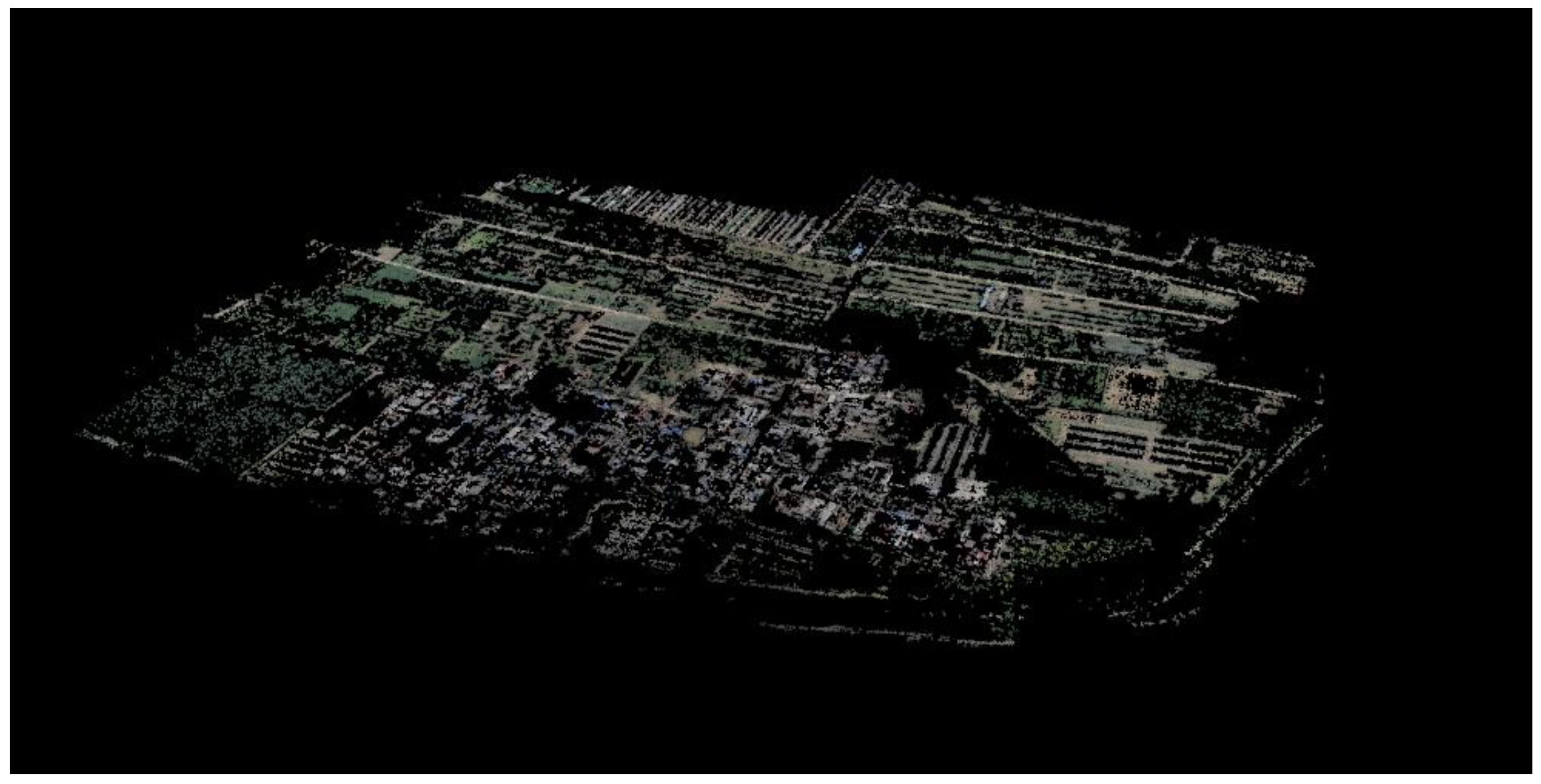
According to the computer three-dimensional visual algorithm, the matched points are handled to generate the sparse point cloud (Figure 10). The sparse point cloud is encrypted to obtain the dense point cloud with a geographical reference, as shown in Figure 11. The missing point cloud problem is the most common phenomenon in the photogrammetric system. The main solution of this study is to use missing area images separately for three-dimensional point cloud construction and select the high-precision and high-density point cloud construction options of Pix4Dmapper. The precision results of orientation points and check points by using the bundle adjustment are shown in Table 4.
Analysis of results from different data sources shows that the RMSE in the orientation point and check point of Data Source A was generally less than that of Data Source B. The RMSE in the plane of Data Source B is more than two times higher than that of Data Source A, and the RMSE in the elevation Data Source B is also more than two times higher than that of Data Source A.
3.3. Analysis of the Tree Information Extraction Method
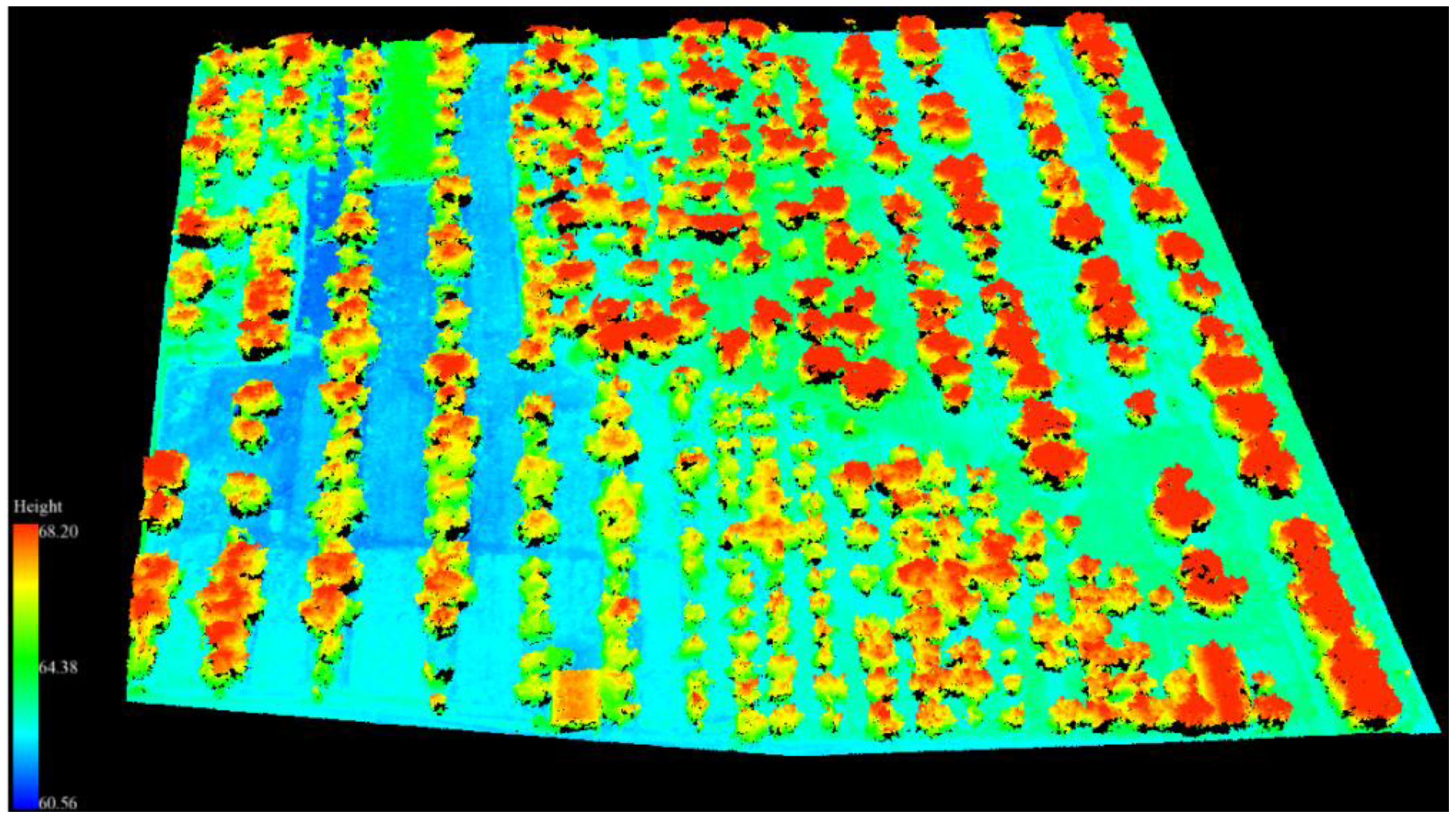
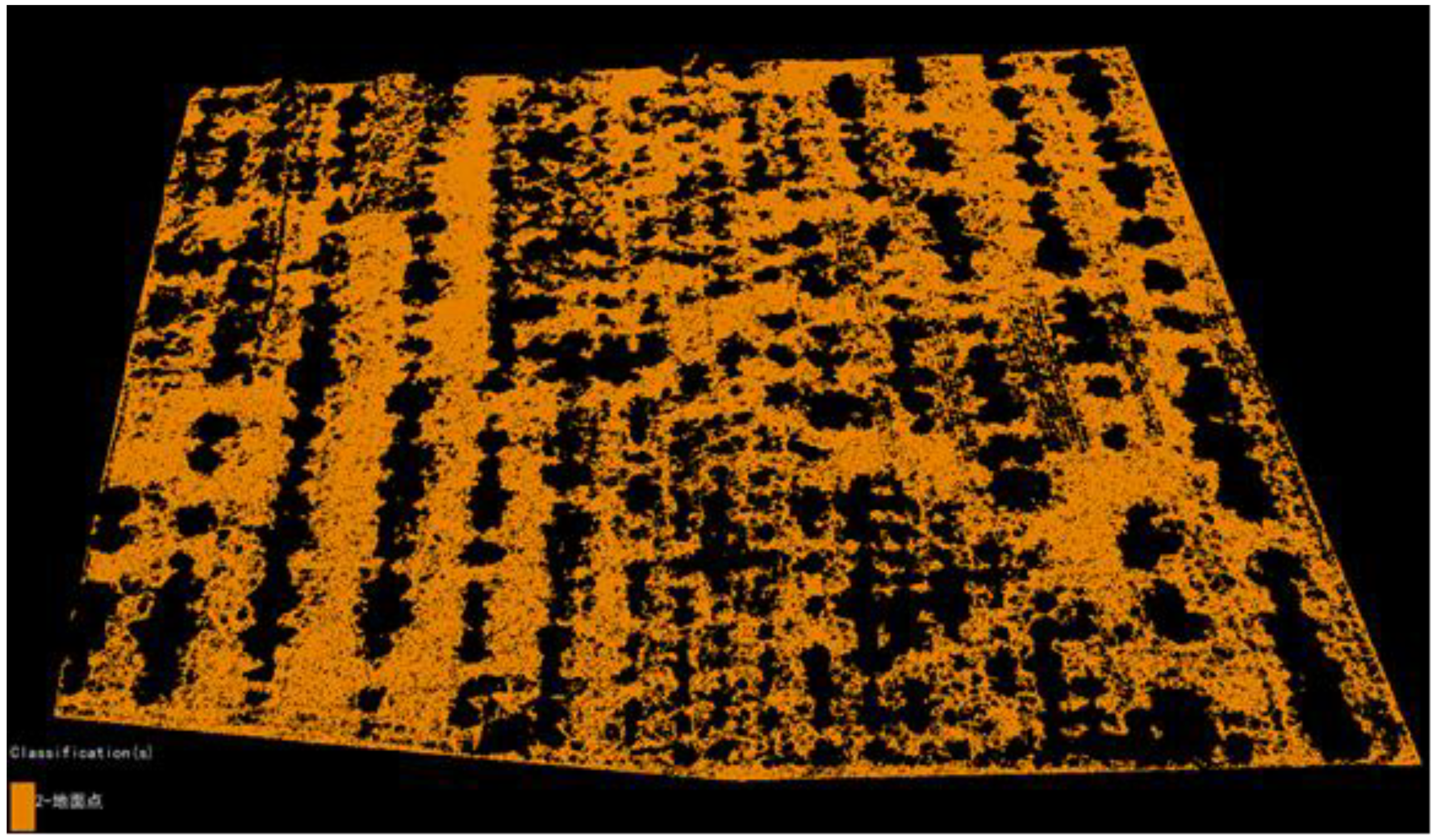
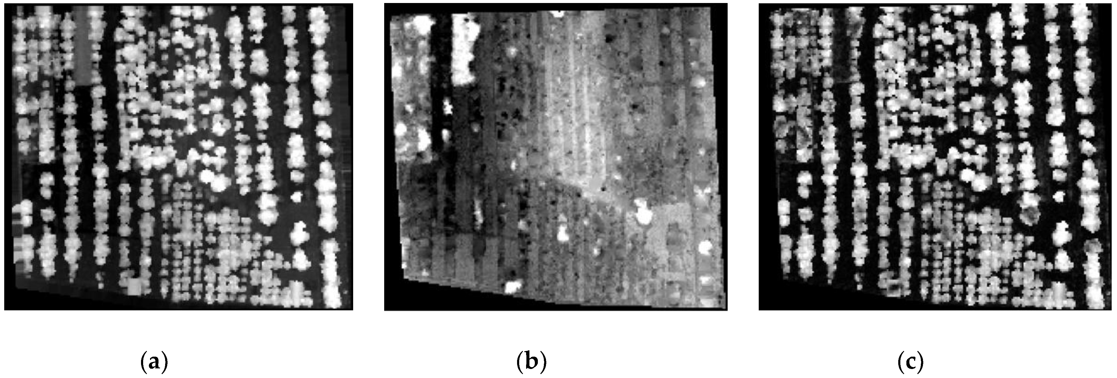
After multiple processing experiments, tree information extraction has the best processing effect by dividing areas (no more than 10 km2). The point cloud data is displayed by the elevation of ancient tree communities, as shown in Figure 12. The classification results of ground points are shown in Figure 13. The DSM (Figure 14a), DEM (Figure 14b), and CHM (Figure 14c) after processing are shown in Figure 14.
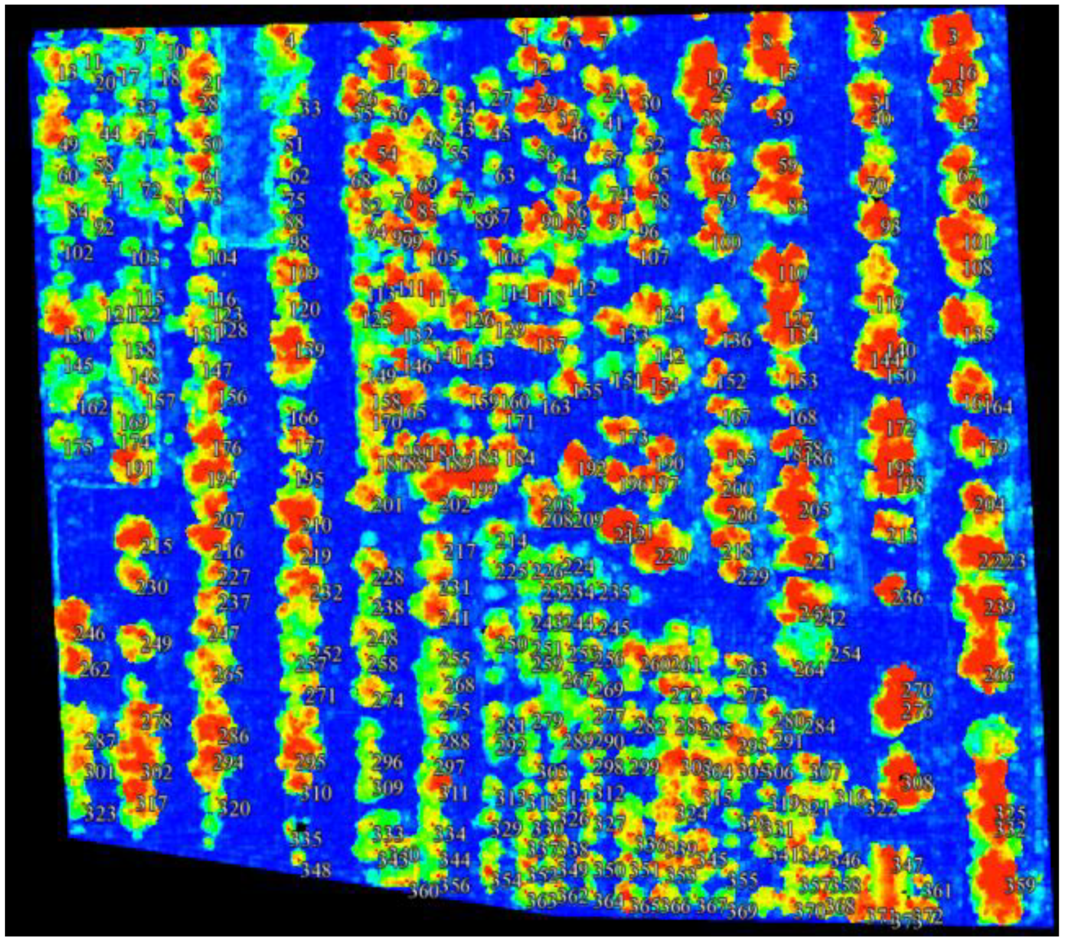
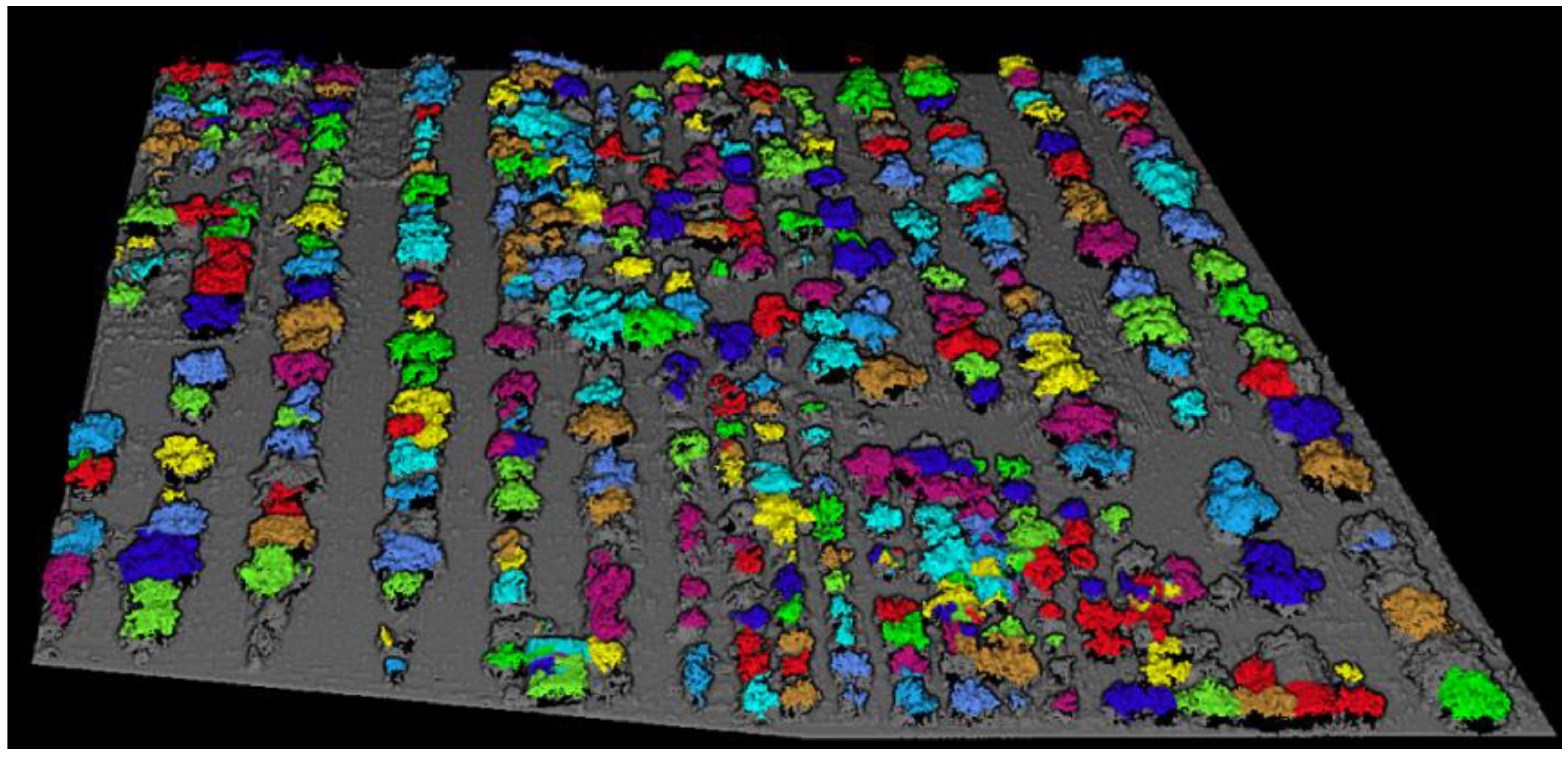
According to the seed points (Figure 15), the prominent position of point cloud data is segmented and the information of individual trees is calculated, as shown in Figure 16.
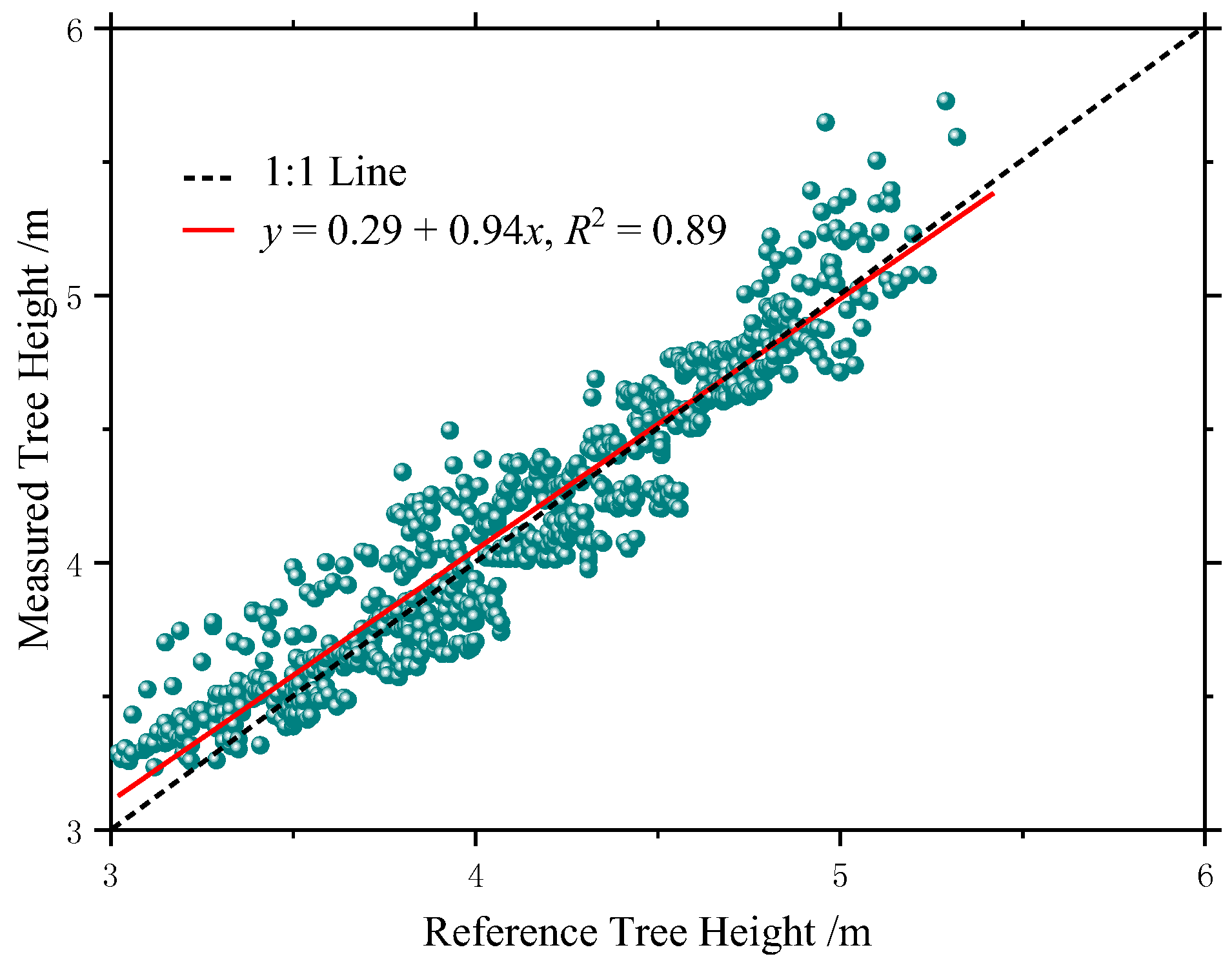
To verify the measurement accuracy of tree height in the system, the reference tree heights of 745 pear trees were arranged from small to large, and the tree number was reset. The tree height was distributed between 3.02 and 5.42 m (Figure 17). The results (Table 5) show that the measured values were distributed on both sides of the reference values, and the maximum measurement error was 0.688 m. Most of the measurement error was within 0.3 m.
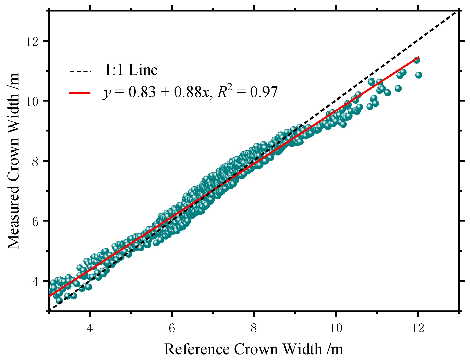
In order to verify the measurement accuracy of the crown width of the system, the reference values of 745 pear trees were arranged according to the size, and the tree number was reset. The canopy amplitude was distributed between 3.01 and 12.02 m (Figure 18). The results (Table 5) show that the measured values are distributed on both sides of the reference value, with the maximum measurement error of 1.165 m. Most of the measurement errors were within 0.5 m.
3.4. Analysis of the Ancient Tree DBH and Age Prediction Model
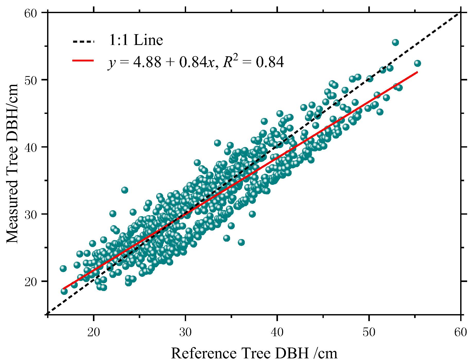
The fitting status of the height–crown-width–DBH model is shown in Table 6. In order to verify the DBH prediction accuracy of the system, the reference values of 745 pear tree data was adjusted according to the size, and the tree number was reset. DBH was distributed between 16.7 and 55.3 cm (Figure 19). The results (Table 7) show that the predicted values were distributed on both sides of the reference value, and the maximum prediction error was 10.33 cm. Most of the prediction errors were within 5 cm.
In the “3 speed 2 inflection points” model, K-means cluster analysis was carried out on the sample data of 39 ancient pear trees, which was divided into three growth stages: 1–26 years as the juvenile period, 27–59 years as the medium period, and ≥60 years as the near-mature period. In addition, the sample of the optimal tree growth index was taken as the mean tree, and the fitting analysis of the “3 speed 2 inflection points” model is shown in Table 8.
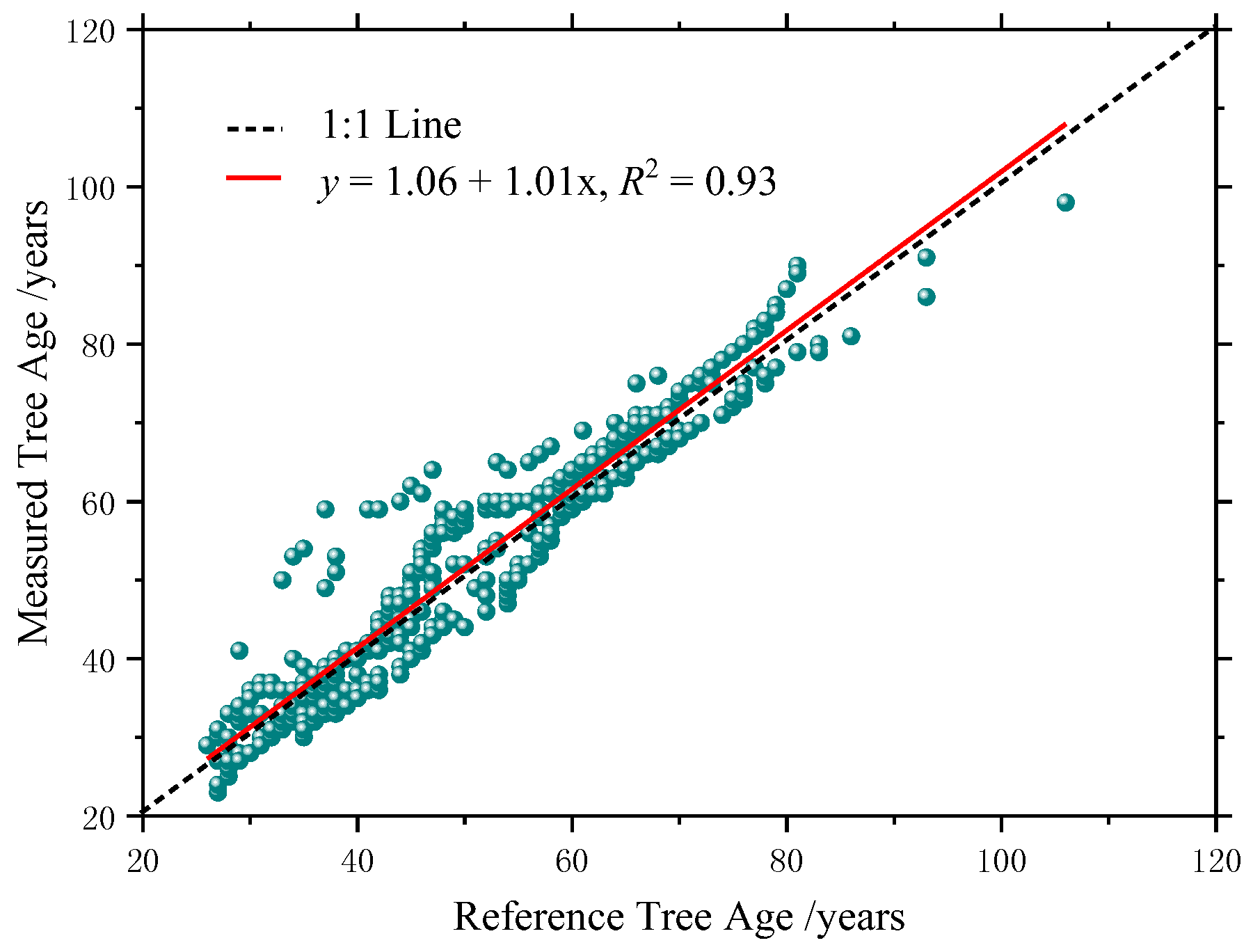
In order to verify the accuracy of the system’s age prediction, the reference ages of 745 pear trees were arranged from small to large, and the tree number was reset, and the ages were distributed between 30 and 104 (Figure 20). The results (Table 9) show that the predicted value is distributed on both sides of the reference value, and the maximum prediction error is 16 years. Most of the prediction errors were within 8 years. The number of pear trees identified through the system was 391, and the number of pear trees sampled through the increment borer was 401.
4. Discussion
4.1. Comparative Analysis of UAV Photogrammetry in Forestry Application
4.1.1. UAV Photogrammetry to Obtain Forest Structure
There are many studies on extracting the scale structure information of single trees by UAV photogrammetry. Dandois and others (2010) used cameras mounted on a kite platform to obtain aerial images of different-age forests and same-age forest and reconstructed 3D point clouds through Ecosynth. Image construction CHM can be used to estimate tree height (R2 > 0.64) [61]. However, the above research differs greatly from the accuracy of the estimated tree height by our improved system, mainly because our fixed-wing UAV platform is relatively stable. Zarco-Tejada and others analyzed the near-infrared images of olive trees obtained by fixed-wing UAVs, conducted 3D construction by Pix4UAV software (Swiss company Pix4D), and obtained tree height information from DSM image construction, which had good correlation with ground measured trees (R2 = 0.83, RMSE = 35 cm) [62]. The above research is very close to the accuracy of the tree height estimation of this system, but there is still a certain gap in accuracy. The main reason is that our system matches and corrects UAV image and POS data before 3D construction, which is also an innovative and important means to improve the accuracy of low-cost UAV photogrammetry. Ni and others obtained northern forest aerial images through a multi-rotor UAV, reconstructed the three-dimensional point cloud images with Agisoft Photoscan, compared and analyzed the photogrammetric CHM and the LiDAR CHM, and found that the soil scale forest was highly correlated (R2 = 0.87, RMSE = 1.9 m) [63]. In the above research, a multi-rotor UAV platform is used, so there is still a certain gap compared to the fixed-wing UAV platform accuracy. In addition, White and others used RSG to perform the three-dimensional construction of high-altitude aerial images (point cloud density is 12.27 points/m2) [64]. Because the side overlap rate is too low, only fore-and-aft overlap images are used to match. Image construction point cloud minus LiDAR DEM obtains a terrain-normalized point cloud and performs hierarchical analysis according to the slope and canopy closure change. The image construction point cloud and the LiDAR point cloud feature quantities are statistically significant, and the DBH is the largest difference. The model result is the same. There is no trend between slope and canopy closure. However, the combination of photogrammetry and LiDAR proposed by the institute provides a direction for the future extraction of forest structures with higher precision.
4.1.2. UAV Photogrammetry to Obtain Topography under Tree Crowns
There are many related studies on UAV photography to measure the terrain under the forest. Dandois and others (2010) used aerial images of different forests and same-age forests for 3D construction [61]. By comparing the image construction point cloud DEM with the LiDAR DEM, it was found that the image construction DEM accuracy is low due to the influence of forest canopy occlusion. Dandois and others (2013) used three-dimensional construction to obtain aerial images of deciduous forest growing seasons and deciduous seasons [65]. By comparing the image construction DEM and the LiDAR DEM in the growing season and the deciduous season, it was found that the DEM accuracy (RMSE is 0.89–3.04 m) in the deciduous season images is higher than that in the growing season (RMSE is 2.49–5.69 m). In the difference value between the image construction DEM and the LiDAR DEM, the forest coverage area has a larger DEM difference value than the non-forest area. Wallace and others used the aeronautical aerial image of Eucalyptus forest for 3D construction. The image construction DEM and the LiDAR DEM generally have little difference (the average difference value is 0.09 m). For the high canopy density area, the image construction DEM is not as accurate as the LiDAR DEM. In view of the investigation of ancient tree community, our system chose to take advantage of UAV photogrammetry to extract DEM. The main reason besides the low cost is that the overall density of the ancient pear tree community (7000-60,000 trees/km2) is small, and the surrounding bare ground is extensive. As a result, the accuracy of image construction DEM is higher.
4.2. Error Analysis of Improved UAV Photogrammetric Measurement System
UAV photogrammetric measurement system is based on studies of SfM-MVS. In the case of tree height and canopy width measurement, errors are caused by all sorts of reasons. As point clouds are scaled, shifted, and rotated into geographic coordinates, the measurement error of each GCP’s three-dimensional position will also bring additional registration errors to SfM-MVS. The objective of the modified UAV image matching and correction algorithm in this paper is to minimize the registration errors of SfM-MVS. SfM-MVS can generate data equivalent to TLS over short distances. However, as the measurement distance increases, the accuracy decreases significantly, which is also the main precision limiting factor of UAV photogrammetric tree measurement system. Reasonable flight height can improve the measurement accuracy.
The difference of contrast and terrain texture can also affect the measurement accuracy of the UAV photogrammetric tree measurement system. SfM-MVS also faces many challenges in the vegetation survey, such as the dynamic nature of vegetation, the complexity of vegetation, and the need of many topographic models to filter out vegetation and restore bare surface spots. Although TLS data can also restore vegetation surfaces, most verified data sets are bare land elevation obtained from TS (total station), differential GPS (global positioning system), and other measurement methods. A UAV photogrammetric tree measurement system uses a variety of vegetation filtering algorithms, classifies pixels according to RGB values with multi-scale dimension standards, resampling point cloud at lower resolution, and finally extracts the minimum observation height in a wide and dense vegetation area. In this process of vegetation filtration, the error will increase with the increase of vegetation density. Because of the low stand density of ancient trees, the error is relatively small in the investigation of the ancient tree community. Moreover, for the purpose of protecting the ancient tree community, the Daxing District Gardening and Greening Bureau regularly processed the other vegetation around the ancient tree. Ancient trees, other trees, and bare land are obviously different from each other in images. Therefore, the UAV photogrammetric tree measurement system can be well used for terrain data extraction.
In addition, due to the large imaging distortion residuals of consumer-grade camera, the aerial triangulation calculation of GCPs may lead to the cumulative diffusion of orientation error. Therefore, choosing medium format cameras, high-precision UAV platforms, and optimizing algorithms can not only significantly reduce the uncertainty of the elements of exterior orientation, but also improve measurement accuracy.
4.3. Error Analysis of the Ancient Tree DBH and Age Prediction Model
Both the growth of DBH and changes in tree rings were influenced by many factors such as climate, environment, and the physiological characteristics of vegetation, especially sensitive to climate change. In the past, the non-linear growth model of trees did not consider factors such as climate and environment. The main reason was that the data source was normal-growth trees, and the purpose was to study the growth curve of the tree. Since ancient pear trees are old, it is difficult to study a growth model by a normal-growth trees method. Forest modeling in this study was combined with UAV photogrammetry to obtain a universal model of the growth of ancient pear trees for the inversion of DBH and tree age. Therefore, by effectively classifying the growth index of each pear tree in the data source, the height–crown-width–DBH model and the “3 Speed 2 Inflection Points” optimum condition growth model can simulate the optimal growth process of ancient pear trees.
There are some uncertainties in the establishment of an ancient tree community model, which is caused by many aspects. There are few studies on the physiological parameters of pear species in China, which makes it unreliable to predict the growth trend of pear trees with their physiological parameters. The model is randomly fitted with its own parameters, which results in a certain amount of error in the accuracy of the simulation results. Due to the lack of climate data in this study, there is no relevant climate data to study the optimal growth process of ancient pear trees, which will reduce the accuracy of the model. In addition, forest modeling in this study also has some limitations, and factors such as external interference activities of the forest ecosystem (such as natural disasters, diseases, and pests) are not taken into account. The improvement of model parameters, the physiological parameters of vegetation, and climate data will increase the accuracy of the model simulation.
The forest modeling experiment results in this paper show that most of the predicted results have good consistency and achieve significant relevant predictions. The variability of individual prediction results is mainly caused by individual differences and special environmental impacts. In addition, the distribution of pear community is relatively scattered, and canopy breadth is less affected by forest density. Therefore, the height–crown-width–DBH model’s precision is high. However, some pear trees are affected by site conditions and disease and insect disasters, which produces large prediction errors. Because a small number of pear trees grow in sandy environments, this results in slow DBH growth. Therefore, the predicted age is much smaller than the actual age, but most pear trees have better accuracy in predicting age. The overall level of precision could meet the demand of the ancient tree community survey.
5. Conclusions
In this study, a UAV photogrammetric measurement system was developed for the investigation of ancient tree communities. Through an improved UAV photogrammetric program and an ancient tree information extraction method, highly efficient and highly precise measurement of tree height and crown width can be achieved. The accurate prediction of DBH and age can be achieved through the construction of a height–crown-width–DBH model and a “3 speed 2 inflection points” optimum condition growth model.
Although the system is aimed at the investigation of ancient tree communities, the improved UAV photogrammetric program and the ancient tree information extraction method can provide a new method for the application of UAV photogrammetry in a forestry survey. In addition, the height–crown-width–DBH model can predict tree diameter with high precision. The study proposed that a “3 speed 2 inflection points” optimum condition growth model based on tree growth index could predict tree age accurately and provide a new method for age identification in a forest survey. Therefore, a UAV photogrammetric tree measurement system can be applied in ancient tree community surveys and even partial forestry surveys. In the future, if forest environment ground monitoring data can be combined, forest modeling research can be improved and achieve the low-cost and high-precision measurement of stand density, stand volume, carbon storage, and biomass.
Author Contributions
Z.Q. and Z.-K.F. conceived and designed the experiments; Z.Q. and M.W. performed the experiments; Z.Q., Z.L., and C.L. analyzed the data; Z.Q. wrote the main manuscript. All authors contributed in writing and discussing the paper.
Funding
This work was supported by the Medium-to-Long-Term Project of Young Teachers’ Scientific Research in Beijing Forestry University (Grant number 2015ZCQ-LX-01), the National Natural Science Foundation of China (Grant number U1710123), and the Beijing Municipal Natural Science Foundation (Grant number 6161001).
Conflicts of Interest
The authors declare no conflict of interest.
Appendix A
Ancient trees are mainly distributed in Panggezhuang Town (Figure A1), Yufa Town (Figure A2), Anding Town (Figure A3), and Zhangziying Town (Figure A4).
Figure A1.
Ancient trees distributed in the Panggezhuang Town.

Figure A2.
Ancient trees distributed in the Yufa Town.

Figure A3.
Ancient trees distributed in the Anding Town.

Figure A4.
Ancient trees distributed in the Zhangziying Town.

References
- Brawn, J.D. Effects of restoring oak savannas on bird communities and populations. Conserv. Biol. 2006, 20, 460–469. [Google Scholar] [CrossRef] [PubMed]
- Gibbons, P.; Lindenmayer, D.; Fischer, J.; Manning, A.; Weinberg, A.; Seddon, J.; Ryan, P.; Barrett, G. The future of scattered trees in agricultural landscapes. Conserv. Biol. 2008, 22, 1309–1319. [Google Scholar] [CrossRef] [PubMed]
- Andersson, M.; Milberg, P.; Bergman, K.-O. Low pre-death growth rates of oak (Quercus robur L.)—Is oak death a long-term process induced by dry years? Ann. For. Sci. 2011, 68, 159–168. [Google Scholar] [CrossRef]
- Lindenmayer, D.B.; Laurance, W.F.; Franklin, J.F. Global decline in large old trees. Science 2012, 338, 1305–1306. [Google Scholar] [CrossRef] [PubMed]
- Buse, J.; Assmann, T.; Friedman, A.L.L.; Rittner, O.; Pavlicek, T. Wood-inhabiting beetles (coleoptera) associated with oaks in a global biodiversity hotspot: A case study and checklist for israel. Insect Conserv. Divers. 2013, 6, 687–703. [Google Scholar] [CrossRef]
- Helama, S.; Vartiainen, M.; Kolström, T.; Peltola, H.; Meriläinen, J. X-ray microdensitometry applied to subfossil tree-rings: Growth characteristics of ancient pines from the southern boreal forest zone in finland at intra-annual to centennial time-scales. Veg. Hist. Archaeobot. 2008, 17, 675–686. [Google Scholar] [CrossRef]
- Briffa, K.R. Annual climate variability in the holocene: Interpreting the message of ancient trees. Quat. Sci. Rev. 2000, 19, 87–105. [Google Scholar] [CrossRef]
- Foody, G.M.; Atkinson, P.M.; Gething, P.W.; Ravenhill, N.A.; Kelly, C.K. Identification of specific tree species in ancient semi-natural woodland from digital aerial sensor imagery. Ecol. Appl. 2005, 15, 1233–1244. [Google Scholar] [CrossRef]
- Qiu, Z.; Feng, Z.; Jiang, J.; Lin, Y.; Xue, S. Application of a continuous terrestrial photogrammetric measurement system for plot monitoring in the Beijing Songshan National Nature Reserve. Remote Sens. 2018, 10, 1080. [Google Scholar] [CrossRef]
- Yan, F.; Ullah, M.R.; Gong, Y.; Feng, Z.; Chowdury, Y.; Wu, L. Use of a no prism Electronic Total Station for field measurements in Pinus tabulaeformis Carr. Stands in china. Biosyst. Eng. 2012, 113, 259–265. [Google Scholar] [CrossRef]
- Qiu, Z.; Feng, Z.; Lu, J.; Sun, R. Design and experiment of forest telescope intelligent dendrometer. Trans. Chin. Soc. Agric. Mach. 2017, 48, 202–207, 213. [Google Scholar]
- Qiu, Z.; Feng, Z.; Jiang, J.; Fan, Y. Design and experiment of forest intelligent surveying and mapping instrument. Trans. Chin. Soc. Agric. Mach. 2017, 48, 179–187. [Google Scholar]
- Van Leeuwen, M.; Nieuwenhuis, M. Retrieval of forest structural parameters using lidar remote sensing. Eur. J. For. Res. 2010, 129, 749–770. [Google Scholar] [CrossRef]
- Liang, X.; Kankare, V.; Hyyppä, J.; Wang, Y.; Kukko, A.; Haggrén, H.; Yu, X.; Kaartinen, H.; Jaakkola, A.; Guan, F. Terrestrial laser scanning in forest inventories. ISPRS J. Photogramm. Remote Sens. 2016, 115, 63–77. [Google Scholar] [CrossRef] [Green Version]
- Murphy, G.E.; Acuna, M.A.; Dumbrell, I. Tree value and log product yield determination in radiata pine (Pinus radiata) plantations in Australia: Comparisons of terrestrial laser scanning with a forest inventory system and manual measurements. Can. J. For. Res. 2010, 40, 2223–2233. [Google Scholar] [CrossRef]
- Pueschel, P.; Newnham, G.; Rock, G.; Udelhoven, T.; Werner, W.; Hill, J. The influence of scan mode and circle fitting on tree stem detection, stem diameter and volume extraction from terrestrial laser scans. ISPRS J. Photogramm. Remote Sens. 2013, 77, 44–56. [Google Scholar] [CrossRef]
- Ryding, J.; Williams, E.; Smith, M.J.; Eichhorn, M.P. Assessing handheld mobile laser scanners for forest surveys. Remote Sens. 2015, 7, 1095–1111. [Google Scholar] [CrossRef]
- Nord-Larsen, T.; Schumacher, J. Estimation of forest resources from a country wide laser scanning survey and national forest inventory data. Remote Sens. Environ. 2012, 119, 148–157. [Google Scholar] [CrossRef]
- Holmgren, J.; Persson, Å. Identifying species of individual trees using airborne laser scanner. Remote Sens. Environ. 2004, 90, 415–423. [Google Scholar] [CrossRef]
- Lim, K.; Treitz, P.; Baldwin, K.; Morrison, I.; Green, J. Lidar remote sensing of biophysical properties of tolerant northern hardwood forests. Can. J. Remote Sens. 2003, 29, 658–678. [Google Scholar] [CrossRef]
- Lim, K.S.; Treitz, P.M. Estimation of above ground forest biomass from airborne discrete return laser scanner data using canopy-based quantile estimators. Scand. J. For. Res. 2004, 19, 558–570. [Google Scholar] [CrossRef] [Green Version]
- Næsset, E. Effects of different flying altitudes on biophysical stand properties estimated from canopy height and density measured with a small-footprint airborne scanning laser. Remote Sens. Environ. 2004, 91, 243–255. [Google Scholar] [CrossRef]
- Patenaude, G.; Hill, R.; Milne, R.; Gaveau, D.; Briggs, B.; Dawson, T. Quantifying forest above ground carbon content using lidar remote sensing. Remote Sens. Environ. 2004, 93, 368–380. [Google Scholar] [CrossRef]
- Leberl, F.; Irschara, A.; Pock, T.; Meixner, P.; Gruber, M.; Scholz, S.; Wiechert, A. Point clouds. Photogramm. Eng. Remote Sens. 2010, 76, 1123–1134. [Google Scholar] [CrossRef]
- Bohlin, J.; Wallerman, J.; Fransson, J.E. Forest variable estimation using photogrammetric matching of digital aerial images in combination with a high-resolution dem. Scand. J. For. Res. 2012, 27, 692–699. [Google Scholar] [CrossRef]
- Järnstedt, J.; Pekkarinen, A.; Tuominen, S.; Ginzler, C.; Holopainen, M.; Viitala, R. Forest variable estimation using a high-resolution digital surface model. ISPRS J. Photogramm. Remote Sens. 2012, 74, 78–84. [Google Scholar] [CrossRef]
- Chiang, K.-W.; Tsai, M.-L.; Chu, C.-H. The development of an uav borne direct georeferenced photogrammetric platform for ground control point free applications. Sensors 2012, 12, 9161–9180. [Google Scholar] [CrossRef] [PubMed]
- Fonstad, M.A.; Dietrich, J.T.; Courville, B.C.; Jensen, J.L.; Carbonneau, P.E. Topographic structure from motion: A new development in photogrammetric measurement. Earth Surf. Process. Landf. 2013, 38, 421–430. [Google Scholar] [CrossRef]
- Dalponte, M.; Bruzzone, L.; Gianelle, D. Fusion of hyperspectral and lidar remote sensing data for classification of complex forest areas. IEEE Trans. Geosci. Remote Sens. 2008, 46, 1416–1427. [Google Scholar] [CrossRef]
- An, N.; Welch, S.M.; Markelz, R.J.C.; Baker, R.L.; Palmer, C.M.; Ta, J.; Maloof, J.N.; Weinig, C. Quantifying time-series of leaf morphology using 2d and 3d photogrammetry methods for high-throughput plant phenotyping. Comput. Electron. Agric. 2017, 135, 222–232. [Google Scholar] [CrossRef]
- Kim, D.; Yun, H.S.; Jeong, S.; Kwon, Y.; Kim, S.; Lee, W.S.; Kim, H. Modeling and testing of growth status for Chinese cabbage and white radish with UAV based rgb imagery. Remote Sens. 2018, 10, 563. [Google Scholar] [CrossRef]
- Kane, V.R.; North, M.P.; Lutz, J.A.; Churchill, D.J.; Roberts, S.L.; Smith, D.F.; McGaughey, R.J.; Kane, J.T.; Brooks, M.L. Assessing fire effects on forest spatial structure using a fusion of landsat and airborne lidar data in yosemite national park. Remote Sens. Environ. 2014, 151, 89–101. [Google Scholar] [CrossRef]
- Zellweger, F.; Braunisch, V.; Baltensweiler, A.; Bollmann, K. Remotely sensed forest structural complexity predicts multi species occurrence at the landscape scale. For. Ecol. Manag. 2013, 307, 303–312. [Google Scholar] [CrossRef]
- Hill, A.; Breschan, J.; Mandallaz, D. Accuracy assessment of timber volume maps using forest inventory data and lidar canopy height models. Forests 2014, 5, 2253–2275. [Google Scholar] [CrossRef]
- St-Onge, B.; Audet, F.-A.; Bégin, J. Characterizing the height structure and composition of a boreal forest using an individual tree crown approach applied to photogrammetric point clouds. Forests 2015, 6, 3899–3922. [Google Scholar] [CrossRef]
- Sankey, T.T.; McVay, J.; Swetnam, T.L.; McClaran, M.P.; Heilman, P.; Nichols, M. Uav hyperspectral and lidar data and their fusion for arid and semi-arid land vegetation monitoring. Remote Sens. Ecol. Conserv. 2018, 4, 20–33. [Google Scholar] [CrossRef]
- Sankey, T.; Donager, J.; McVay, J.; Sankey, J.B. Uav lidar and hyperspectral fusion for forest monitoring in the southwestern USA. Remote Sens. Environ. 2017, 195, 30–43. [Google Scholar] [CrossRef]
- Corona, P.; Fattorini, L. Area-based lidar-assisted estimation of forest standing volume. Can. J. For. Res. 2008, 38, 2911–2916. [Google Scholar] [CrossRef] [Green Version]
- Steinmann, K.; Mandallaz, D.; Ginzler, C.; Lanz, A. Small area estimations of proportion of forest and timber volume combining lidar data and stereo aerial images with terrestrial data. Scand. J. For. Res. 2013, 28, 373–385. [Google Scholar] [CrossRef]
- Næsset, E. Predicting forest stand characteristics with airborne scanning laser using a practical two-stage procedure and field data. Remote Sens. Environ. 2002, 80, 88–99. [Google Scholar] [CrossRef]
- Lisein, J.; Pierrot-Deseilligny, M.; Bonnet, S.; Lejeune, P. A photogrammetric workflow for the creation of a forest canopy height model from small unmanned aerial system imagery. Forests 2013, 4, 922–944. [Google Scholar] [CrossRef]
- Lee, H.; Slatton, K.C.; Roth, B.E.; Cropper, W., Jr. Adaptive clustering of airborne lidar data to segment individual tree crowns in managed pine forests. Int. J. Remote Sens. 2010, 31, 117–139. [Google Scholar] [CrossRef]
- Kaartinen, H.; Hyyppä, J.; Yu, X.; Vastaranta, M.; Hyyppä, H.; Kukko, A.; Holopainen, M.; Heipke, C.; Hirschmugl, M.; Morsdorf, F. An international comparison of individual tree detection and extraction using airborne laser scanning. Remote Sens. 2012, 4, 950–974. [Google Scholar] [CrossRef] [Green Version]
- Li, W.; Guo, Q.; Jakubowski, M.K.; Kelly, M. A new method for segmenting individual trees from the lidar point cloud. Photogramm. Eng. Remote Sens. 2012, 78, 75–84. [Google Scholar] [CrossRef]
- Gonzalez-Benecke, C.; Gezan, S.A.; Samuelson, L.J.; Cropper, W.P.; Leduc, D.J.; Martin, T.A. Estimating Pinus palustris tree diameter and stem volume from tree height, crown area and stand-level parameters. J. For. Res. 2014, 25, 43–52. [Google Scholar] [CrossRef]
- Carrer, M.; Urbinati, C. Age-dependent tree-ring growth responses to climate in Larix decidua and Pinus cembra. Ecology 2004, 85, 730–740. [Google Scholar] [CrossRef]
- Climent, J.; Chambel, M.; Pérez, E.; Gil, L.; Pardos, J. Relationship between heartwood radius and early radial growth, tree age, and climate in Pinus canariensis. Can. J. For. Res. 2002, 32, 103–111. [Google Scholar] [CrossRef]
- Othman, M.F.; Shazali, K. Wireless sensor network applications: A study in environment monitoring system. Procedia Eng. 2012, 41, 1204–1210. [Google Scholar] [CrossRef]
- Carrivick, J.L.; Smith, M.W.; Quincey, D.J. Structure from Motion in the Geosciences; John Wiley & Sons: Chichester, UK, 2016. [Google Scholar]
- Smith, M.; Carrivick, J.; Quincey, D. Structure from motion photogrammetry in physical geography. Prog. Phys. Geogr. 2016, 40, 247–275. [Google Scholar] [CrossRef]
- Mosbrucker, A.R.; Major, J.J.; Spicer, K.R.; Pitlick, J. Camera system considerations for geomorphic applications of sfm photogrammetry. Earth Surf. Process. Landf. 2017, 42, 969–986. [Google Scholar] [CrossRef]
- McLauchlan, P.F.; Jaenicke, A. Image mosaicing using sequential bundle adjustment. Image Vis. Comput. 2002, 20, 751–759. [Google Scholar] [CrossRef] [Green Version]
- Chow, J.C.; Lichti, D.D. Photogrammetric bundle adjustment with self-calibration of the primesense 3d camera technology: Microsoft kinect. IEEE Access 2013, 1, 465–474. [Google Scholar] [CrossRef]
- Mouragnon, E.; Lhuillier, M.; Dhome, M.; Dekeyser, F.; Sayd, P. Generic and real-time structure from motion using local bundle adjustment. Image Vis. Comput. 2009, 27, 1178–1193. [Google Scholar] [CrossRef] [Green Version]
- Di, K.; Liu, Y.; Liu, B.; Peng, M.; Hu, W. A self-calibration bundle adjustment method for photogrammetric processing of chang ’E-2 stereo lunar imagery. IEEE Trans. Geosci. Remote Sens. 2014, 52, 5432–5442. [Google Scholar]
- Schnabel, R.; Wahl, R.; Klein, R. Efficient Ransac for Point-Cloud Shape Detection; Computer Graphics Forum; Wiley Online Library: Oxford, UK, 2007; pp. 214–226. [Google Scholar]
- Dobbertin, M. Tree growth as indicator of tree vitality and of tree reaction to environmental stress: A review. Eur. J. For. Res. 2005, 124, 319–333. [Google Scholar] [CrossRef]
- Zeide, B. Analysis of growth formulas. For. Sci. 1993, 39, 594–616. [Google Scholar]
- Weiner, J.; Thomas, S.C. The nature of tree growth and the “age-related decline in forest productivity”. Oikos 2001, 94, 374–376. [Google Scholar] [CrossRef]
- Moulia, B.; Coutand, C.; Lenne, C. Posture control and skeletal mechanical acclimation in terrestrial plants: Implications for mechanical modeling of plant architecture. Am. J. Bot. 2006, 93, 1477–1489. [Google Scholar] [CrossRef] [PubMed]
- Dandois, J.P.; Ellis, E.C. Remote sensing of vegetation structure using computer vision. Remote Sens. 2010, 2, 1157–1176. [Google Scholar] [CrossRef]
- Zarco-Tejada, P.J.; Diaz-Varela, R.; Angileri, V.; Loudjani, P. Tree height quantification using very high resolution imagery acquired from an unmanned aerial vehicle (uav) and automatic 3d photo-reconstruction methods. Eur. J. Agron. 2014, 55, 89–99. [Google Scholar] [CrossRef]
- Ni, W.; Liu, J.; Zhang, Z.; Sun, G.; Yang, A. Evaluation of UAV-Based Forest Inventory System Compared with Lidar Data. In Proceedings of the 2015 IEEE International Geoscience and Remote Sensing Symposium (IGARSS), Milan, Italy, 26–31 July 2015; pp. 3874–3877. [Google Scholar]
- White, J.C.; Stepper, C.; Tompalski, P.; Coops, N.C.; Wulder, M.A. Comparing als and image-based point cloud metrics and modelled forest inventory attributes in a complex coastal forest environment. Forests 2015, 6, 3704–3732. [Google Scholar] [CrossRef]
- Dandois, J.P.; Ellis, E.C. High spatial resolution three-dimensional mapping of vegetation spectral dynamics using computer vision. Remote Sens. Environ. 2013, 136, 259–276. [Google Scholar] [CrossRef]
Figure 1.
Layout of the research area.

Figure 2.
The scene of ancient trees investigation.

Figure 3.
YS-500 Fixed-Wing Unmanned Aerial Vehicle (UAV).

Figure 4.
SIFT algorithm image matching the partial region (blue “+” represents feature points that match between images).
Figure 4.
SIFT algorithm image matching the partial region (blue “+” represents feature points that match between images).

Figure 5.
Image correction of the free network adjustment in ancient tree communities.

Figure 6.
Selection and positioning of the image control points.

Figure 7.
Image correction of the regional system adjustment of ancient tree communities.

Figure 8.
Layout scheme.

Figure 9.
Digital surface model (DSM) and digital elevation model (DEM) schematic.

Figure 10.
Sparse 3D point cloud of ancient tree communities.

Figure 11.
Dense 3D point cloud of ancient tree communities.

Figure 12.
Point cloud data displayed by elevation of ancient tree communities.

Figure 13.
Ground point classification of ancient tree communities.

Figure 14.
The DSM (a), DEM (b), and canopy height model (CHM) (c) of ancient tree communities.

Figure 15.
Seed point generated in ancient tree communities.

Figure 16.
Eye-dome lighting (EDL) display of ancient tree communities.

Figure 17.
Reference value and measured value distribution of tree height.

Figure 18.
Reference value and measured value distribution of tree crown width.

Figure 19.
Reference value and measured value distribution of DBH.

Figure 20.
Reference value and measured value distribution of tree age.


Table 1.
Parameters of YS-500 Fixed-Wing UAV.
| Content | Parameters Value |
|---|---|
| Wingspan | 1700 mm |
| Length | 900 mm |
| Dynamical System | Dynamoelectric system |
| Materials | Aeronautical Composite |
| Maximum Take-off Weight | 5.5 kg |
| Aircraft Standard Load | 1.5 kg |
| Speed | 70–120 km/h |
| Cruising Speed | 80–90 km/h |
| Maximum Flying Distance | 100 km |
| Cruising Range | 80 km |
| Cruising Duration | 90 min |
| Maximum Flying Altitude | 4500 m |
| Wind Resistance | 10.8–13.8 m/s |
| Working Temperature | −10 °C–50 °C |
| Radio Range | 30 km |
Table 2.
Calibration parameters of the Sony-A7R camera (measurement by the Chinese Academy of Surveying and Mapping).
Table 2.
Calibration parameters of the Sony-A7R camera (measurement by the Chinese Academy of Surveying and Mapping).
| Calibration Content | Calibration Value |
|---|---|
| Principal Point x0 | −0.188561 |
| Principal Point y0 | −0.138128 |
| Focal Length f | 36.289444 mm |
| Pixel Size | 4.88 μm |
| Picture Format (pixel) | 7360 × 4912 |
| Coefficient of Radial Distortion k1 | −5.145797 × 10⁻⁵ |
| Coefficient of Radial Distortion k2 | 1.583367 × 10⁻⁷ |
| Coefficient of Radial Distortion k3 | 1.829755 × 10⁻⁵ |
| Tangential Distortion Factor p1 | −6.050453 × 10⁻⁶ |
| Tangential Distortion Factor p2 | −1.739164 × 10⁻⁵ |
Table 3.
Specific parameters of Yinhe I RTK (Real Time Kinematic) measurement system (measurement by the China South Surveying & Mapping Instrument Company).
Table 3.
Specific parameters of Yinhe I RTK (Real Time Kinematic) measurement system (measurement by the China South Surveying & Mapping Instrument Company).
| Instrument Specifications | Specific Parameters |
|---|---|
| Signal Tracking | 220 signal channel |
| BDS B1, B2, B3 | |
| GPS L1C/A, L1C, L2C, L2E, L5 | |
| GLONASS L1C/A, L1P, L2C/A, L2P, L3 | |
| SBAS L1C/A, L5 | |
| Galileo GIOVE-A, and GIOVE-B, E1, E5A, E5B | |
| QZSS, WAAS, MSAS, EGNOS, GAGAN (Veripos) | |
| GNSS Features | Positioning output frequency, 1 Hz–50 Hz |
| Initialization time, Less than 10 s | |
| Able to support GNSS constellation signals from all current and future plans | |
| High reliable carrier tracking technology | |
| Intelligent dynamic sensitivity positioning technology | |
| High precision positioning processing engine | |
| Differential positioning accuracy | Horizontal: 0.25 m + 1 ppm RMS |
| Vertical: 0.50 m + 1 ppm RMS | |
| SBAS differential positioning accuracy: Typical <5m 3DRMS | |
| Static GNSS measurements | ±(2.5 mm + 1 mm/km × d), d is the distance of the measured point, km |
| Real-time dynamic measurement (RTK) | ±(8 mm + 1 mm/km × d), d is the distance of the measured point, km |
Table 4.
Aerial triangulation accuracy for different data sources.
| Data Sources | Data Source A | Data Source B | |
|---|---|---|---|
| Fundamental orientation points | RMSE of plane | 0.233 m | 0.442 m |
| Maximum error of plane | 0.317 m | 0.762 m | |
| RMSE of elevation | 0.154 m | 1.516 m | |
| Maximum error of elevation | 0.196 m | 2.289 m | |
| Check points | RMSE of plane | 0.299 m | 0.314 m |
| Maximum error of plane | 0.691 m | 0.714 m | |
| RMSE of elevation | 0.873 m | 1.508 m | |
| Maximum error of elevation | 1.498 m | 2.686 m | |
Table 5.
Verification and analysis of measurement accuracy of tree height and crown width.
| RMSE | RMSE% | Bias | Bias% | |
|---|---|---|---|---|
| Tree Height (m) | 0.1814 m | 4.39% | 0.0408 m | 0.99% |
| Crown width (m) | 0.3292 m | 4.73% | 0.0244 m | 0.35% |
Table 6.
Fitting analysis of the height–crown-width– diameter-at-breast-height (DBH) model ().
| Factor | Estimated Value | Standard Error | Lower Limit of 95% Confidence Interval | Upper Limit of 95% Confidence Interval |
|---|---|---|---|---|
| 1.570 | 0.193 | 1.191 | 1.950 | |
| 1.428 | 0.052 | 1.325 | 1.530 | |
| 2.296 | 0.242 | 1.821 | 2.771 | |
| 1.119 | 0.035 | 1.051 | 1.187 |
Table 7.
Accuracy analysis of DBH prediction.
| RMSE | RMSE% | Bias | Bias% | |
|---|---|---|---|---|
| DBH (cm) | 3.0039 cm | 9.25% | −0.4193 cm | −1.29% |
Table 8.
Fitting analysis of “3 speed 2 inflection points” model ().
| Factor | Estimated Value | Standard Value | Lower Limit of 95% Confidence Interval | Upper Limit of 95% Confidence Interval |
|---|---|---|---|---|
| 26.959 | 0.747 | 25.494 | 28.424 | |
| 12.076 | 0.455 | 11.184 | 12.969 | |
| 0.522 | 0.035 | 0.453 | 0.590 | |
| 25.907 | 0.866 | 24.208 | 27.605 | |
| 1.341 | 0.054 | 1.236 | 1.447 | |
| 74.661 | 3.330 | 68.131 | 81.191 | |
| 5.739 | 1.778 | 2.207 | 9.272 | |
| 1.326 | 0.521 | 0.290 | 2.361 | |
| 1.147 | 0.006 | 1.135 | 1.159 |
Table 9.
Age prediction accuracy analysis.
| RMSE | RMSE% | Bias | Bias% | |
|---|---|---|---|---|
| Tree Age/years | 4.3753 years | 8.77% | 1.5141 years | 3.03% |
© 2018 by the authors. Licensee MDPI, Basel, Switzerland. This article is an open access article distributed under the terms and conditions of the Creative Commons Attribution (CC BY) license (http://creativecommons.org/licenses/by/4.0/).
Share and Cite
MDPI and ACS Style
Qiu, Z.; Feng, Z.-K.; Wang, M.; Li, Z.; Lu, C. Application of UAV Photogrammetric System for Monitoring Ancient Tree Communities in Beijing. Forests 2018, 9, 735. https://doi.org/10.3390/f9120735
AMA Style
Qiu Z, Feng Z-K, Wang M, Li Z, Lu C. Application of UAV Photogrammetric System for Monitoring Ancient Tree Communities in Beijing. Forests. 2018; 9(12):735. https://doi.org/10.3390/f9120735
Chicago/Turabian StyleQiu, Zixuan, Zhong-Ke Feng, Mingming Wang, Zhenru Li, and Chao Lu. 2018. "Application of UAV Photogrammetric System for Monitoring Ancient Tree Communities in Beijing" Forests 9, no. 12: 735. https://doi.org/10.3390/f9120735
Note that from the first issue of 2016, this journal uses article numbers instead of page numbers. See further details here.